1. Background
Given a set of n points in , and an error parameter , a coreset in this paper is a small set of weighted points in , such that the sum of squared distances from the original set of points to any set of k centers in can be approximated by the sum of weighted squared distances from the points in the coreset. The output of running an existing clustering algorithm on the coreset would then yield approximation to the output of running the same algorithm on the original data, by the definition of the coreset.
Coresets were first suggested by [
1] as a way to improve the theoretical running time of existing algorithms. Moreover, a coreset is a natural tool for handling
using all the computation models that are mentioned in the previous section. This is mainly due to the merge-and-reduce tree approach that was suggested by [
2,
3] and is formalized by [
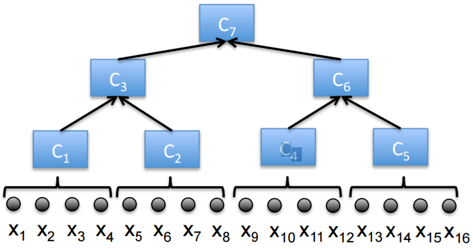
4]: coresets can be computed independently for subsets of input points, e.g., on different computers, and then be merged and re-compressed again. Such a binary compression tree can also be computed using one pass over a possibly unbounded streaming set of points, where in every moment only
coresets exist in memory for the
n points streamed so far. Here the coreset is computed only on small chunks of points, so a possibly inefficient coreset construction still yields efficient coreset constructions for large sets; see
Figure 1. Note that the coreset guarantees are preserved while using this technique, while no assumptions are made on the order of the streaming input points. These coresets can be computed independently and in parallel via
M machines (e.g., on the cloud) and reduce the running time by a factor of
M. The communication between the machines is also small, since each machine needs to communicate to a main server only the coreset of its data.
In practice, this technique can be implemented easily using the map-reduce approach of modern software for
such as [
5].
Coresets can also be used to support the dynamic model where points are deleted/inserted. Here the storage is linear in
n since we need to save the tree in memory (practically, on the hard drive), however the update time is only logarithmic in
n since we need to reconstruct only
coresets that correspond to the deleted/inserted point along the tree. First such coreset of size
independent of
d was introduced by [
6]. See [
1,
2] for details.
Constrained k-Means and Determining k
Since the coreset approximates every set of
k centers, it can also be used to solve the
k-means problem under different constraints (e.g., allowed areas for placing the centers) or given a small set of candidate centers. In addition, the set of centers may contain duplicate points, which means that the coreset can approximate the sum of squared distances for
centers. Hence, coresets can be used to choose the right number
k of centers up to
, by minimizing the sum of squared distances plus
for some function of
k. Full opensource is available [
8].
2. Related Work
We summarize existing coresets constructions for
k-means queries, as will be formally defined in
Section 4.
Importance Sampling
Following a decade of research, coreset of size polynomial in
d were suggested by [
9]. Ref [
10] suggested an improved version of size
in which is a special case of the algorithms proposed by [
11]. The construction is based on computing an approximation to the
k-means of the input points (with no constraints on the centers) and then sample points proportionally to their distance to these centers. Each chosen point is then assigned a weight that is inverse proportional to this distance. The probability of failure in these algorithms reduces exponentially with the input size. Coresets of size
, i.e., linear in
k, were suggested in work of [
12], however the weight of a point may be negative or a function of the given query. For the special case
, Inaba et al. [
13], provided constructions of coresets of size
using uniform sampling.
Projection based coresets. Data summarization which are similar to coresets of size
that are based on projections on low-dimensional subspaces that diminishes the sparsity of the input data were suggested by [
14] by improving the analysis of [
4]. Recently [
15] improves both on [
4,
14] by applying Johnson-Lindenstrauss Lemma [
16] on construction from [
4]. However, due to the projections, the resulting summarizations of all works mentioned above are not subset of the input points, unlike the coreset definition of this paper. In particular, for sparse data sets such as adjacency matrix of a graphs, documents-term matrix of Wikipedia, or images-objects matrix, the sparsity of the data diminishes and a single point in the summarization might be larger than the complete sparse input data.
Other type of weak coresets approximates only the optimal solution, and not every
k centers. Such randomized coresets of size independent of
d and only polynomial in
k were suggested by [
11] and simplified by [
12].
Deterministic Constructions. The first coresets for
k-means [
2,
17] were based on partitioning the data into cells, and take a representative point from each cell to the coreset, as is done in hashing or Hough transform [
18]. However, these coresets are of size at least
, i.e., exponential in
d, while still providing result which is a sub-set of the the input in contrast to previous work [
17]. While, our technique is most related to the deterministic construction that was suggested in [
4] by recursively computing
k-means clustering of the input points. While the output set has size independent of
d, it is not a coreset as defined in this paper, since it is not a subset of the input and thus cannot handle sparse data as explained above. Techniques such as uniform sampling for each cluster yields coresets with probability of failure that is linear in the input size, or whose size depends on
d.
m-means is a coreset for k-means? A natural approach for coreset construction, that is strongly related to this paper, is to compute the
m-means of the input set
P, for a sufficiently large
m, where the weight of each center is the number of point in its cluster. If the sum of squared distances to these
m-centers is about
factor from the
k-means, we obtain a
-coreset by (a weaker version of) the triangle inequality. Unfortunately, it was recently proved in [
19] that there exists sets such that
centers are needed in order to obtain this small sum of squared distances.
3. Our Contribution
We suggest the following deterministic algorithms:
An algorithm that computes a approximation for the k-means of a set P that is distributed (partitioned) among M machines, where each machine needs to send only input points to the main server at the end of its computation.
A streaming algorithm that, after one pass over the data and using
memory returns an
-approximation to the
k-means of
P. The algorithm can run “embarrassingly in parallel [
20] on data that is distributed among
M machines, and support insertion/deletion of points as explained in the previous section.
Description of how to use our algorithm to boost both the running time and quality of any existing k-means heuristic using only the heuristic itself, even in the classic off-line setting.
Extensive experimental results on real world data-sets. This includes the first k-means clustering with provable guarantees for the English Wikipedia, via 16 EC2 instances on Amazon’s cloud.
Open-code for for fully reproducing our results and for the benefit of the community. To our knowledge, this is the first coreset code that can run on the cloud without additional commercial packages.
3.1. Novel Approach: m-Means Is A Coreset for k-Means, for Smart Selection of m
One of our main technical result is that for every constant
, there exists an integer
such that the
m-means of the input set (or its approximation) is a
-coreset; see Theorem 2. However, simply computing the
m-means of the input set for a sufficiently large
m might yield
m that is exponential in
d, as explained by [
19] and the related work. Instead, Algorithm 1 carefully selects the right
m between
k and
after checking the appropriate conditions in each iteration.
3.2. Solving k-Means Using k-Means
It might be confusing that we suggest to solve the k-means problem by computing m-means for . In fact, most of the coreset constructions actually solve the optimal problem in one of their first construction steps. The main observation is that we never run the coreset on the complete input of n (or unbounded stream of) points, but only on small subsets of size . This is since our coresets are composable and can be merged (to points) and reduced back to m using the merge-and-reduce tree technique. The composable property follows from the fact that the coreset approximates the sum of squared distances to every k-centers, and not just the k-means for the subset at hand.
3.3. Running Time
Running time that is exponential in
k is unavoidable for any
-approximation algorithm that solves
k-means, even in the planar case
[
21] and
[
4]. Our main contributions is a coreset construction that uses memory that is independent of
d and running time that is
near-linear in
n. To our knowledge this is an open problem even for the case
. Nevertheless, for large values of
(e.g.,
) we may use existing constant factor approximations that takes time polynomial in
k to compute our coreset in time that is near-linear in
n but also polynomial in
k.
In practice, provable -approximations for k-means are rarely used due to the lower bounds on the running times above. Instead, heuristics are used. Indeed, in our experimental results we evaluate this approach instead of computing the optimal k-means during the coreset construction and on the resulting coreset itself.
4. Notation and Main Result
The input to our problem is a set of n points in , where each point includes a multiplicative weight . In addition, there is an additive weight for the set. Formally, a weighted set in is a tuple , where , . In particular, an unweighted set has a unit weight for each point, and a zero additive weight.
4.1. k-Means Clustering
For a given set
of
centers (points) in
, the Euclidean distance from a point
to its closest center in
Q is denoted by 1.7
em. The sum of these weighted squared distances over the points of
P is denoted by
If P is an unweighted set, this cost is just the sum of squared distances over each point in to its closest center in Q.
Let denote the subset of points in whose closest center in Q is , for every . Ties are broken arbitrarily. This yields a partition of by Q. More generally, the partition of P by Q is the set where , and for every and every .
A set
that minimizes this weighted sum
over every set
Q of
k centers in
is called the
k-means of
P. The 1-means
of
P is called the centroid, or the center of mass, since
We denote the cost of the k-means of P by .
4.2. Coreset
Computing the
k-means of a weighted set
P is the main motivation of this paper. Formally, let
be an error parameter. The weighted set
is a
-coreset for
P, if for every set
of
centers we have
To handle streaming data we will need to compute “coresets for union of coresets”, which is the reason that we assume that both the input P and its coreset S are weighted sets.
4.3. Sparse Coresets
Unlike previous work, we add the constraints that if each point in P is sparse, i.e., has few non-zeroes coordinates, then the set S will also be sparse. Formally, the maximum sparsity of P is the maximum number of non zeroes entries over every point p in P.
In particular, if each point in S is a linear combination of at most points in P, then . In addition, we would like that the set S will be of size independent of both and d.
We can now state the main result of this paper.
Theorem 1 (Small sparse coreset). For every weighted set in , and an integer , there is a -coreset of size where each point in is a linear combination of points from . In particular, the maximum sparsity of is .
By plugging this result to the traditional merge-and-reduce tree in
Figure 1, it is straight-forward to compute a coreset using one pass over a stream of points.
Corollary 1. A coreset of size and maximum sparsity can be computed for the set P of the n points seen so far in an unbounded stream, using memory words. The insertion time per point in the stream is . If the stream is distributed uniformly to M machines, then the amortized insertion time per point is reduced by a (multiplicative) factor of M to . The coreset for the union of streams can then be computed by communicating the M coresets to a main server.
5. Coreset Construction
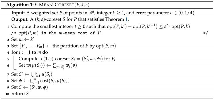
Our main coreset construction algorithm k gets a set P as input, and returns a -coreset ; see Algorithm 1.
To obtain running time that is linear in the input size, without loss of generality, we assume that
P has
points, and that the cardinality of the output
S is
. This is thanks to the traditional merge-and-reduce approach: given a stream of
n points, we apply the coreset construction only on subsets of size
from
P during the streaming and reduce them by half. See
Figure 1 and e.g., [
4,
7] for details.
Algorithm Overview
In Line 1 we compute the smallest integer
such that the cost
of the
m-means of
P is close to the cost
of the
-means of
P. In Line 3 we compute the corresponding partition
of
P by its
m-means
. In Line 5 a
-sparse coreset
of size
is computed for every
,
. This can be done deterministically e.g., by taking the mean of
as explained in Lemma 1 or by using a gradient descent algorithm, namely Frank-Wolfe, as explained in [
22] which also preserves the sparsity of the coreset as desired by our main theorem. The output of the algorithm is the union of the means of all these coresets, with appropriate weight, which is the size of the coreset.
The intuition behind the algorithm stems from the assumption that m-means clustering will have lower cost than
k-means and this is actually supported by series of previous work [
23,
24]. In fact our experiments in
Section 7 evidence that in practice it actually works better than anticipated by theoretical bounds.
6. Proof of Correctness
The first lemma states the common fact that the sum of squared distances of a set of point to a center is the sum of their squared distances to their center of mass, plus the squared distance to the center (the variance of the set).
Proof. The last term equals zero since
, and thus
The second lemma shows that assigning all the points of P to the closest center in Q yields a small multiplicative error if the 1-mean and the k-means of P has roughly the same cost. If , this means that we can approximate using only one center in the query; see Line 1 of Algorithm 1. Note that for .
Lemma 2. For every set of centers we have Proof. Let
denote a center that minimizes
over
. The left inequality of (
1) is then straight-forward since
It is left to prove the right inequality of (
1). Indeed, for every
, let
denote the closest point to
p in
Q. Ties are broken arbitrarily. Hence,
Let
denote the partition of
P by
, where
are the closest points to
for every
; see
Section 4. For every
, let
. Hence,
where in (4) and (5) we substituted
and
respectively in Lemma 1, and in (6) we use the fact that
and
for every
. Summing (6) over
yields
To bound (8), we substitute
and then
in Lemma 1, and obtain that for every
where the last inequality is by the definition of
. This implies that for every
,
Plugging the last inequality in (8) yields
where (11) is by Cauchy-Schwartz inequality, and in (12) we use the fact that
for every
.
To bound the left term of (13) we use the fact
and substitute
,
in Lemma 1 for every
as follows.
To bound the right term of (13) we use
to obtain
Plugging (
14) and the last inequality in (13) yields
Together with (
2) this proves Lemma 2. □
Lemma 3. Let S be a -coreset for a weighted set P in . Let be a finite set. Then Proof. Let
be a center such that
, and let
be a center such that
. The right side of (
15) is bounded by
where the first inequality is by the optimality of
, and the second inequality is since
S is a coreset for
P. Similarly, the left hand side of (
15) is bounded by
where the last inequality follows from the assumption
. □
Lemma 4. Let S be the output of a call to k. Then S is a -coreset for P.
Proof. By replacing
P with
in Lemma 1 for each
it follows that
Summing the last inequality over each
yields
Since
is the partition of the
m-means of
P we have
. By letting
be the
m-means of
we have
Hence,
where the second inequality is by Line 1 of the algorithm. Plugging the last inequality in (
16) yields
Using Lemma 3, for every
By summing over
we obtain
Plugging the last inequality in (
17) yields
Hence, S is a coreset for P. □
Lemma 5. There is an integer such that Proof. Contradictively assume that (
19) does not hold for every integer
. Hence,
Contradiction, since . □
Using the mean of in Line 5 of the algorithm yields a -coreset as shown in Lemma 1. The resulting coreset is not sparse, but gives the following result.
Theorem 2. There is such that the m-means of P is a -coreset for P.
Proof of Theorem 1. We compute
a
mean coreset for 1-mean of
at line 5 of Algorithm 1 by using variation of Frank-Wolfe [
22] algorithm. It follows that
for each
i, therefore the overall sparsity of
S is
. This and Lemma 4 concludes the proof. □
7. Comparison to Existing Approaches
In this section we provide experimental results of our main algorithm of coreset constructions. We compare the clustering with existing coresets and small/medium/large datasets. Unlike most of the coreset papers, we also run the algorithm on the distributed setting via a cloud as explained below.
7.1. Datasets
For our experimental results we use three well known datasets, and the English Wikipedia as follows.
MNIST handwritten digits [25]. The MNIST dataset consists of
grayscale images of handwritten digits. Each image is of size 28 × 28 pixels and was converted to a row vector row of
dimensions.
Pendigits [26]. This dataset was downloaded from the UCI repository. It consists of 250 written letters by 44 humans. These humans were asked to write 250 digits in a random order inside boxes of 500 by 500 tablet pixel resolution. The tablet sends
x and
y tablet coordinates and pressure level values of the pen at fixed time intervals (sampling rate) of 100 milliseconds. Digits are represented as constant length feature vectors of size
the number of digits in the dataset is
.
NIPS dataset [
27]. The OCR scanning of NIPS proceedings over 13 years. It has 15,000 pages and 1958 articles. For each author, there is a corresponding words counter vector, where the
ith entry in the vector is the number of the times that the word used in one of the author’s submissions. There are overall
authors and
words in this corpus.
English Wikipedia [28]. Unlike previous datasets that were uploaded to memory and then compressed via streaming coresets, the English Wikipedia practically can not be uploaded completely to memory. The size of the dataset is 15GB after converting to a term-documents matrix via gensim [
29]. It has 4M vectors, each of
dimensions and an average of 200 non-zero entries, i.e., words per document.
7.2. The Experiment
We applied our coreset construction to boost the performance of Lloyd’s
k-means heuristic as explained in
Section 8 of previous work [
6]. We compared the results with the current data summarization algorithms that can handle sparse data: uniform and importance sampling.
7.3. On the Small/Medium Datasets
We evaluate both the offline computation and the streaming data model. For offline computation we used the datasets above to produce coresets of size
, then computed
k-means for
till convergence. For the streaming data model, we divided each dataset into small subsets and computed coresets via the merge-and-reduce technique to construct a coreset tree as in
Figure 1. Here, the coresets are smaller, of size
, and the values for
k-means are the same.
We computed the sum of squared distances to the original (full) set of points, from each resulting set of k centers that was computed from the coreset. These sets of centers are denoted by and for uniform, non uniform sampling and our coreset respectively. The “ground truth” or “optimal solution” was computed using k-means on the entire dataset until convergence. The empirical estimated error was then defined to be for coreset number . Note that, since Lloyd’s k-means is a heuristic, its performance on the reduced data might be better, i.e., .
These experiments were run on a single common laptop machine with 2.2GHz quad-core Intel Core i7 CPU and 16GB of 1600MHz DDR3L RAM with 256GB PCIe-based onboard SSD.
7.4. On the Wikipedia Dataset
We compared the three discussed data summarization techniques, while each one was computed in parallel and in a distributed fashion on 16 EC2 virtual servers. We repeated computation for and 128, and coresets size in the range .
This experiment was executed via Amazon’s Web Services (“cloud”), using 16 EC2 virtual computation nodes of type c4.4xlarge, which 8 vCPU and 15GiB of RAM. We repeated distributed computation evaluating for coresets of sizes 256, 512, 1024 and 2048 points for k-means with .
7.5. Results
The results of experiment for
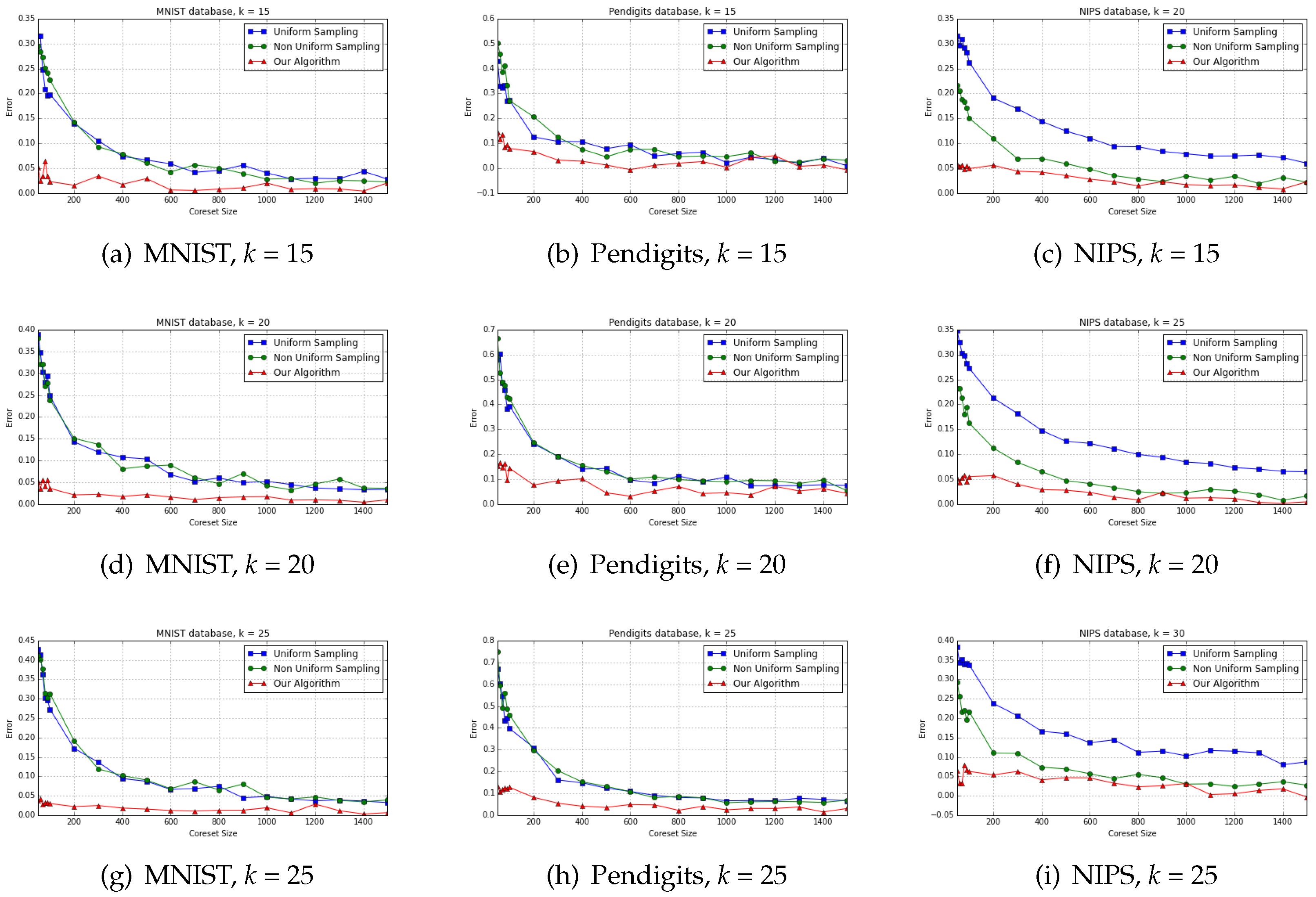
on small datasets for offline computation are depicted on
Figure 2, where it’s evident that error of kmeans computation fed by our coreset algorithm results outperforms error of uniform and non-uniform sampling.
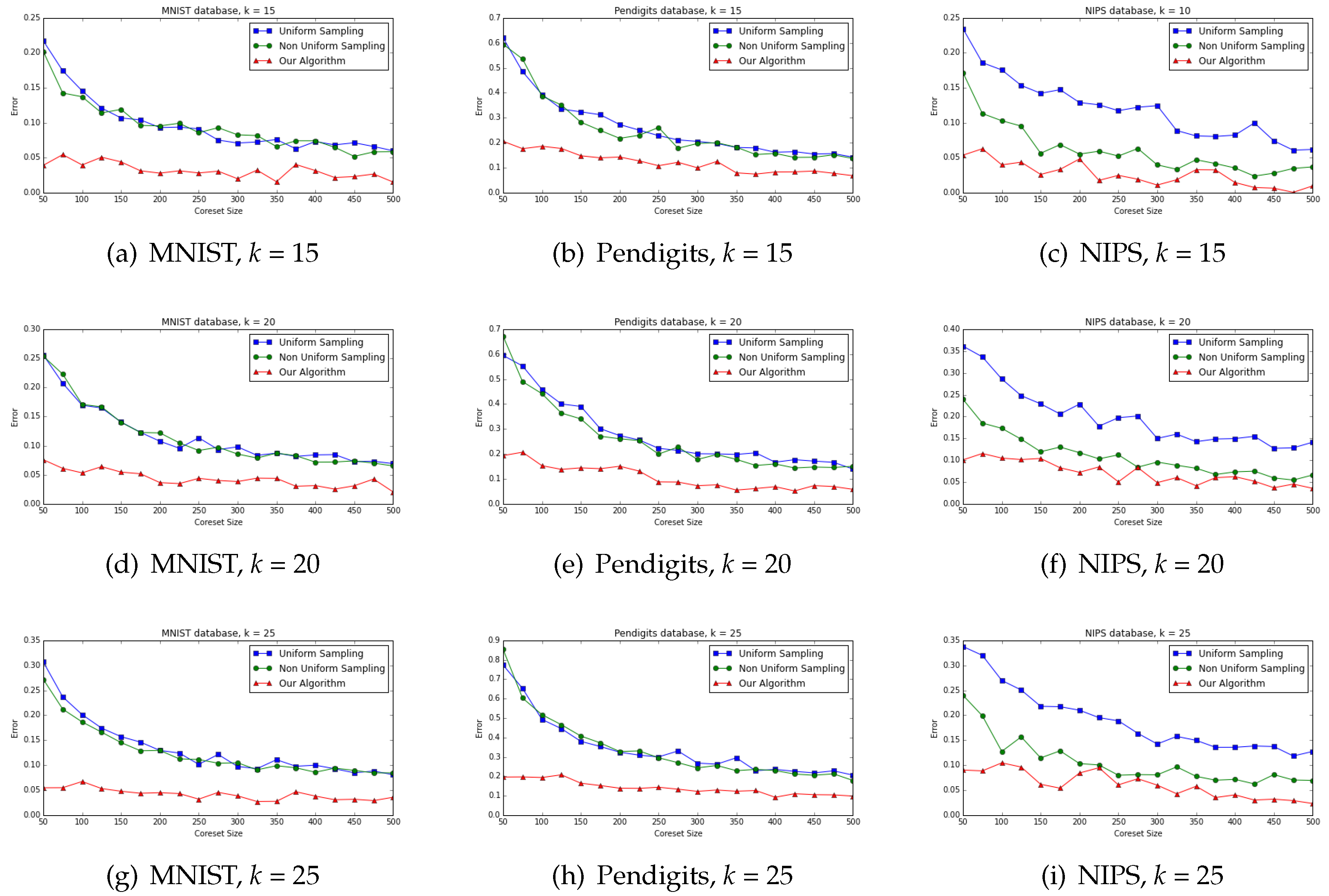
For streaming computation model our algorithm is able to provide results which are better than other two as could be explored in
Figure 3. In addition, existing algorithms suffer from “cold start” as common in random sampling techniques: there is a slow convergence to the small error, compared to our deterministic algorithm that introduces small error already after a small sample size.
At
Figure 4 presented results of the experiment on Wikipedia dataset for different values of
, as it could be easily observed proposed coreset algorithm provides good results of big sparse dataset and provides lower energy cost compared to uniform and non-uniform approaches.
Figure 5,
Figure 6 and
Figure 7 show the box-plot of error distribution for all the three coresets in the offline and streaming settings. Our algorithm shows a little variance across all experiments, its mean error is very close to its median error, indicating that it produces stable results.
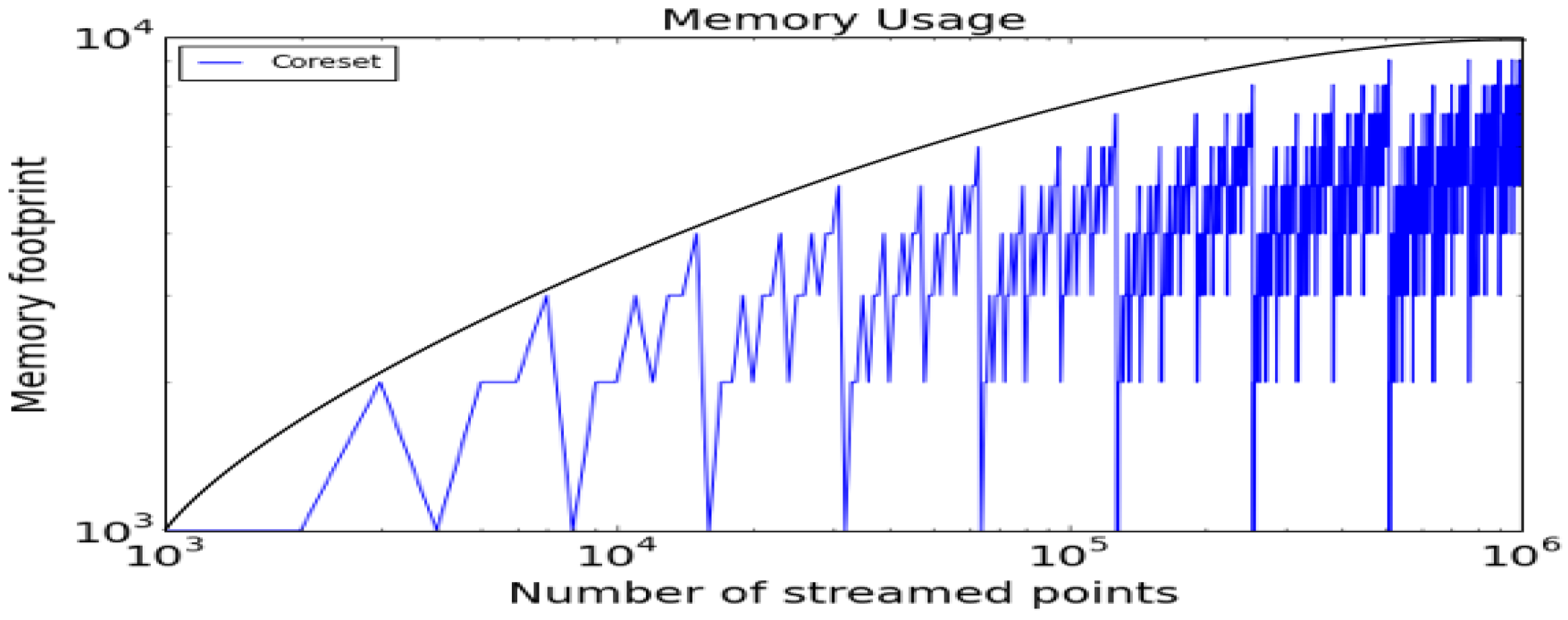
Figure 8 shows the memory (RAM) footprint during the coreset construction based on synthetically generated random data. The oscillations corresponds to the number of coresets in the tree that each new subset needs to update. For example, the first point in a streaming tree is updated in
, however the
th point for some
climbs up through
levels in the tree, so
coresets are merged.
8. Conclusions
We proved that any set of points in has a -coreset which consists of a weighted subset of the input points whose size is independent of n and d, and polynomial in . Our algorithm carefully selects m such that the m-means of the input with appropriate weights (clusters’ size) yields such a coreset.
This allows us to finally compute coreset for sparse high dimensional data, in both the streaming and the distributed setting. As a practical example, we computed the first coreset for the full English Wikipedia. We hope that our open source code will allow researchers in the industry and academia to run these coresets on more databases such as images, speech or tweets.
The reduction to k-means allows us to use popular k-means heuristics (such as Lloyd-Max) and provable constant factor approximations (such as k-means++) in practice. Our experimental results on both a single machine and on the cloud shows that our coreset construction significantly improves over existing techniques, especially for small coresets, due to its deterministic approach.
We hope that this paper will also help the community to answer the following three open problems:
- (i)
Can we simply compute the m-means for a specific value and obtain a -coreset without using our algorithm?
- (ii)
Can we compute such a coreset (subset of the input) whose size is ?
- (iii)
Can we compute such a smaller coreset deterministically?
