Article

Distributional Reinforcement Learning with Ensembles

Department of Mathematics, Linnæus University, 351 95 Växjö, Sweden
*
Author to whom correspondence should be addressed.
Algorithms 2020, 13(5), 118; https://doi.org/10.3390/a13050118
Submission received: 8 April 2020 / Revised: 23 April 2020 / Accepted: 30 April 2020 / Published: 7 May 2020
(This article belongs to the Section Evolutionary Algorithms and Machine Learning)

Abstract

:
It is well known that ensemble methods often provide enhanced performance in reinforcement learning. In this paper, we explore this concept further by using group-aided training within the distributional reinforcement learning paradigm. Specifically, we propose an extension to categorical reinforcement learning, where distributional learning targets are implicitly based on the total information gathered by an ensemble. We empirically show that this may lead to much more robust initial learning, a stronger individual performance level, and good efficiency on a per-sample basis.

1. Introduction

The fact that ensemble methods may outperform single agent algorithms in reinforcement learning has been demonstrated numerous times [1,2,3,4]. These methods can involve combining several algorithms into one agent and then taking actions by a weighted aggregation scheme or rank voting. However, most conventional ensemble methods in reinforcement learning are often based on expected returns. Perhaps the simplest example is the average joint policy derived from an ensemble of independently trained agents, where the action of the ensemble is dictated by the average of the estimated Q-values of each agent.
An alternate view to that of Q-values, the distributional perspective on state-action returns, was discussed in [5]. This paradigm represents a shift of focus towards estimating or using underlying distributions of random return variables instead of learning expectations. This in turn paints a complex and more informationally dense picture, and there exists overwhelming empirical evidence that the distributional perspective is helpful in deep reinforcement learning. That is, apart from the possibility of overall stronger performance, algorithmic benefits may also involve the reduction of prediction variance, more robust learning with additional regularization effects, and a larger set of auxiliary goals such as learning risk-sensitive policies [5,6,7,8,9]. Moreover, there have recently been important theoretical works done on understanding the observed improvements and providing theoretical results on convergence [5,9,10,11].
In this paper, we propose a group-aided training scheme for distributional reinforcement learning, where we merge the distributional perspective with an ensemble method involving agents learning in separate environments. Our main contribution in this regard is the proposed Ensemble Categorical Control procedure (ECCprocedure). As an initial study, we also provide empirical results where an ECCalgorithm is tested on a subset of Atari 2600 games [12], which are standard environments for testing these types of algorithms.
Specifically, ECC is an extension of Categorical Distributional Reinforcement Learning (CDRL), which was introduced in [5] and made explicit in [10]. Similar to CDRL, we consider distributions defined on a fixed discrete support, with projections onto the support for all possible categorical distributions arising internally in the algorithm. For each agent in ECC, we replace the target generation of CDRL by targets generated by the ensemble mean mixture distribution of the individual target distributions.
We argue that ECC implies an implicit sharing of information between agents during learning, where the distributional paradigm gives us more robust targets and an arguably more nuanced aggregated picture, which preserves multimodality. The experiments confirm the validity of the approach, where in all cases, the extension generates strong individual agents and good efficiency when regarded as an ensemble.
The paper is organized in the following way. In Section 2, we give a background to distributional reinforcement learning. In Section 3, we introduce the proposed ECCprocedure. At the end of Section 3, we give a reference to another contribution of the present work: the pseudocode and source code for an implementation of the ECCalgorithm. In Section 4, we present and evaluate the results of our implementation of the ECCalgorithm on five specific Atari 2600 environments. Finally, in Section 5, we zoom out and discuss the results in a broader context, as well as suggest future work.

2. Background

We considered agent-environment interactions. For each observed state, the agent selects an action, whereby the environment generates a reward and a next state. Following the framework of [10], we let X and A denote the sets of states and actions, respectively, and let p : X × A P ( R × X ) be a transition kernel that maps state-action pairs to joint distributions of immediate rewards and next states. Then, we can model this interaction by a Markov Decision Process (MDP) ( X , A , p , γ ) , where  γ [ 0 , 1 ) is a discount factor of future rewards. Moreover, an agent can sample its actions through a stationary policy π : X P ( A ) , which maps a current state to a distribution over available actions.
Throughout the rest of this paper, we consider MDPs where X × A is a countable state-action space. We denote by D = P ( R ) X × A the set of functions where η D maps each state-action pair ( x , a ) to a distribution η ( x , a ) P ( R ) . Similarly, we put D n = P n ( R ) X × A , where P n ( R ) is the set of probability distributions with finite n th -moments. For a given η D , we let Q η : X × A R denote the function that maps state-action pairs { ( x , a ) } to the corresponding first moments of { η ( x , a ) } , i.e.,
Q η ( x , a ) R z η ( x , a ) ( d z ) .
To appreciate a subsequent summary of distributional reinforcement theory fully, we may also need to make the following definition explicit.
Definition 1.
For a Borel measurable function g : R R and ν P ( R ) , we let g # ν denote the push-forward measure defined by:
g # ν ( A ) : = ν g 1 ( A )
on all Borel sets A R . In particular, given r , γ R , we let ( f r , γ ) # ν be the push-forward measure where f r , γ ( x ) : = r + γ x .
Suppose further that we have a set P of categorical distributions supported on a fixed set z = { z 1 , z 2 , , z K } of equally-spaced numbers. Then, the following projection operator minimizes the distance between any categorical distribution ν = i = 1 n p i δ y i and elements in P with respect to the Cramér metric [9,13].
Definition 2.
The Cramér projection Π z maps any Dirac measure δ y to a distribution in P by:
Π z ( δ y ) = δ z 1 y z 1 , z i + 1 y Δ z δ z i + y z i Δ z δ z i + 1 z i < y z i + 1 , δ z K y > z K .
Moreover, the projection is defined to be linear over mixture distributions such that:
Π z i p i δ y i = p i Π z δ y i .

2.1. Expected Reinforcement Learning

Before we go into the distributional perspective, let us first give a quick reminder about some value function fundamentals, here stated in operator form.
Let ( X , A , p , γ ) be an MDP. Given ( x , a ) X × A , we define the return of a policy π as the random variable:
Z π ( x , a ) : = t = 0 γ t R t | X 0 = x , A 0 = a ,
where ( R t ) t = 0 is a random sequence of immediate rewards, indexed by time step t and dependent on random state-action pairs ( X t , A t ) t = 0 under p and π .
In an evaluation setting of some fixed policy π , let Q π : X × A R be the expected return function, which by definition has values:
Q π ( x , a ) = E [ Z π ( x , a ) ] .
If we consider distributions dictated by p and π and let R ( x , a ) and ( X , A ) denote the random reward and subsequent random state-action pair given ( x , a ) X × A , then we recall the Bellman operator T π defined by:
( x , a ) T π g ( x , a ) = E p [ R ( x , a ) ] + γ E p , π [ g ( X , A ) ]
on bounded real functions g B ( X × A , R ) . Moreover, in the search for values attained by optimal policies, we also recall the optimality operator T where:
( x , a ) T g ( x , a ) = E p [ R ( x , a ) ] + γ E p [ max a g ( X , a ) ] .
It is readily verified that both operators are contraction maps on the complete metric space B ( X × A , R ) , d . In addition, their unique fixed points are given by Q π and Q , respectively, where Q is the optimal function defined by:
Q ( x , a ) = max π Q π ( x , a )
for all ( x , a ) [14].

2.2. Distributional Reinforcement Learning

We now proceed by presenting some of the main ideas of distributional reinforcement learning in a tabular setting. We will first look at the evaluation problem, where we are trying to find the state-action value of a fixed policy π . Second, we consider the control problem, where we try to find the optimal state-action value. Third, we consider the distributional approximation procedure CDRL used by agents in this paper.

2.2.1. Evaluation

We consider a distributional variant of (2), the distributional Bellman operator given by T π : D D ,
( x , a ) T π η ( x , a ) : = R ( x , a ) X × A ( f r , γ ) # η ( x , a ) π ( a x ) p ( d r , x x , a ) .
Here, T π is, for all n 1 , a γ -contraction in D n with a unique fixed point when D n is endowed with the supremum n th -Wasserstein metric ([5], Lemma 3) (see [15] for more details on Wasserstein distances). Moreover by Proposition 2 of [9], T π is expectation preserving when we have an initial coupling with the T π -iteration given in (2); that is, given an initial η 0 D and a function g, such that g = Q η 0 . Then, T π n g = Q T π n η 0 holds for all n 0 .
Thus, if we let η π D be the function of distributions of Z π in (1), then η π is the unique fixed point satisfying the distributional Bellman equation:
η π = T π η π .
It follows that iterating T π on any starting collection η 0 with bounded moments eventually solves the evaluation task of π to an arbitrary degree.

2.2.2. Control

Recall the Bellman optimality operator T of (3). If we define a corresponding distributional optimality operator T : D D ,
( x , a ) ( T η ) ( x , a ) : = R ( x , a ) X × A ( f r , γ ) # η ( x , a ( x ) ) p ( d r , x x , a ) ,
where a ( x ) = arg max a A Q η ( x , a ) , then expectation values generated by iterates under T will behave as expected. That is, if we put Q n : = Q ( T ) n η 0 , then we have an exponentially fast uniform convergence Q n Q as n . However, T is not a contraction in any metric over distributions and may lack fixed points altogether in D [5].

2.2.3. Categorical Evaluation and Control

In most real applications, the updates of (4) and (5) are either computationally infeasible or impossible to fully compute due to p being unknown. It follows that approximations are key to defining practical distributional algorithms. This could involve parametrization over some selected set of distributions along with projections onto these distributional subspaces. It could also involve stochastic approximations with sampled transitions and gradient updates with function approximation.
A structure for algorithms making use of such approximations is Categorical Distributional Reinforcement Learning (CDRL). In what follows is a short summary of the CDRL procedure fundamental to single agent implementations in this paper.
Let z = { z 1 , z 2 , , z K } be an ordered fixed set of equally-spaced real numbers such that z 1 < z 2 < < z K with Δ z z i + 1 z i . Let:
P = i = 1 K p i δ z i : p 1 , , p K 0 , i = 1 K p i = 1 P ( R )
be the subset of categorical distributions in P ( R ) supported on z . We consider parameterized distributions by using D ^ = P A × X as the collection of possible inputs and outputs of an algorithm. Moreover, for each η D ^ , we have:
Q η ( x , a ) = i = 1 K p i ( x , a ) z i .
as its Q-value function.
Given a subsequent treatment of our extension of CDRL, we first reproduce the steps of the general procedure in Algorithm 1 (see [10], Algorithm 1).
Algorithm 1: Categorical Distributional Reinforcement Learning (CDRL)
  • At each iteration step t and input η t D ^ , sample a transition ( x t , a t , r t , x t ) .
  • Select a to be either sampled from π ( x t ) in the evaluation setting or taken as a = arg max a Q η t ( x t , a ) in the control setting.
  • Recall the Cramér projection Π z given in Definition 2, and put:
    η ^ t ( x t , a t ) : = Π z f r t # η t ( x t , a ) .
  • Take the next iterated function as some update η t + 1 such that:
    KL η ^ t ( x t , a t ) η t + 1 x t , a t < KL η ^ t ( x t , a t ) η t x t , a t ,
    where:
    KL ( p q ) : = i = 1 K p i log p i q i
    denotes the Kullback–Leibler divergence.
Consider first a finite MDP and a tabular setting. Define η ^ t ( x , a ) η t ( x , a ) whenever ( x , a ) ( x t , a t ) . Then, by the convexity of log ( z ) , it is readily verified that updates of the form:
η t + 1 = ( 1 α t ) η t + α t η ^ t ( α t ( 0 , 1 ) )
satisfy Step 4. In fact, if there exists a unique policy π associated with the convergence of (3), then this update yields an almost sure convergence, with respect to the supremum-Cramér metric, to a distribution in D ^ with π as the greedy policy (with some additional assumptions on the stepsizes α t and sufficient support (see [10], Theorem 2, for details).
In practice, we are often forced to use function approximation of the form:
η ( x , a ) = ϕ ( x , a ; θ ) ,
where ϕ is parameterized by some set of weights θ . Gradient updates with respect to θ can then be made to minimize the loss:
KL η ^ t ( x t , a t ) ϕ x t , a t ; θ ,
where η ^ t ( x t , a t ) = Π z f r t # ϕ ( x t , a ; θ fixed ) is the computed learning target of the transition ( x t , a t , r t , x t ) . However convergence with the Kullback–Leibler loss and function approximation is still an open question. Theoretical progress has been made when considering other losses, although we may lose the stability benefits coming from the relative ease of minimizing (6) [9,11,16].
An algorithm implementing CDRL with function approximation is C51 [5]. It essentially uses the same neural network architecture and training procedure as DQN [17]. To increase stability during training, this also involves sampling transitions from an experience buffer and maintaining an older, periodically updated, copy of the weights for target computation. However, instead of estimating Q-values, C51 uses a finite support z of 51 points and learns discrete probability distributions ϕ ( x , a ; θ ) over z via soft-max transfer. Training is done by using the KL-divergence as the loss function over batches with computed targets η ^ ( x , a ) of CDRL.

3. Learning with Ensembles

3.1. Ensembles

Ensemble methods have been widely used in both supervised learning and reinforcement learning. In supervised learning, this can involve bootstrap aggregating predictors for better accuracy when given unstable processes such as neural networks or using “expert” opinion mixtures for better estimators [18,19]. A simple example that demonstrates the possible benefits of aggregation is the following average pool of k regression models: Given a sample to predict, assume that the models draw prediction errors ε i , i = 1 , , k from a zero-mean multivariate normal distribution with E [ ε i 2 ] = σ 2 and correlations ρ i j = ρ . Then, the error made by averaging their predictions is ε : = ( 1 / k ) i = 1 k ε i with:
E [ ε 2 ] = 1 + ρ ( k 1 ) σ 2 k .
It follows that the mean squared error goes to σ 2 / k as ρ 0 , whereas we get σ 2 and no benefit when the errors are perfectly correlated.
Under the assumption of independently trained agents, we have a reinforcement learning variant of the average pool in the following definition.
Definition 3.
Given an ensemble of k agents, let Q ^ ( i ) denote the Q-value function estimate of agent i, and let Q ^ : = ( 1 / k ) i = 1 k Q ^ ( i ) denote the mean function. Then, the average joint policy π ¯ selects actions according to:
a = arg max a Q ^ ( x , a ) = arg max a 1 k i = 1 k Q ^ ( i ) ( x , a ) .
at every x X .
Thus, π ¯ represents an aggregation strategy where we consider the information provided by each agent as equally important. Moreover, by the linearity of expectations and in view of (3), if we have initial functions Q 0 ( i ) with n-step ensemble values Q n : = ( 1 / k ) i = 1 k Q n ( i ) , then full updates Q n ( i ) : = T Q n 1 ( i ) of each agent will yield Q n = T Q n 1 for the ensemble. Assume further that learning is done with a single algorithm in separate environments. If we take Q ^ ( i ) ( x , a ) as estimates of Q n ( i ) ( x , a ) for some step n, with errors ε i distributed as multivariate Gaussian noise, then we should expect Q ^ ( x , a ) to have a smaller expected error variance in its estimation of Q n ( x , a ) similar to regression models. This implies more robust performance when given an unstable training process far from convergence, but it also implies diminishing improvements when the algorithm is close to converging to a unique policy.
However, in real applications, and in particular with function approximation, there may be instances where the improved performance by π ¯ does not vanish due to agents converging to distinct sub-optimal policies. An illustration of this phenomenon can be seen in Figure 1. It shows evaluations during learning in the LunarLander-v2 environment [20]. The single agents used CDRL on a 29 atom support. To approximate distributions, the agents used small neural networks with three encoding layers consisting of 16 units each. The architecture was purposely chosen to make it harder for the optimizer to converge to an optimal policy, possibly due to lack of capacity. At each evaluation point, the models were tested with ε = 0.001 . The figure also includes evaluations of average joint policies of five agents having the same evaluation ε . However, we can see that the joint information provided by an ensemble of five agents transcends individual capacity, indicating that some agents settle on distinct sub-optimal solutions.

3.2. Ensemble Categorical Control

We consider an ensemble of k agents, each independently trained with the same distributional algorithm, where η i , i = 1 , , k are their respective distributional collections. There are several ways to aggregate distributional information provided by the ensemble with respect to forecasts and risk-sensitivity [21,22]. Perhaps the simplest is a distributional variant of the average joint policy, where we consider the mean function η ¯ of mixture distributions:
( x , a ) η ¯ ( x , a ) : = 1 k i = 1 k η i ( x , a ) .
Since η ¯ ( x , a ) is a linear pool, it preserves multimodality during aggregation. Hence, it maintains an arguably more nuanced picture of estimated future rewards compared to methods that generate unimodal aggregations around unrealizable expected values. In addition, expectations under η ¯ yield the Q-function used by the average joint policy in Definition 3 with all the performance benefits that this entails during learning.
The finite support of the CDRL procedure may provide another reason to aggregate by η ¯ : Under the assumption that η i ( x , a ) , i = 1 , , k are drawn as random vectors from some multivariate normal population with mean μ ( x , a ) and covariance Σ ( x , a ) , then η ¯ is a maximum likelihood estimate of the mean categorical distribution μ ( x , a ) induced by the algorithm over all possible training runs [23]. It follows that η ¯ may provide more robust estimates in reflecting mean t-step capabilities of the procedure in terms of distributions found by sending k .
It then stands to reason that (7) should help accelerate learning by providing better and more robust targets in the control setting of CDRL. This implies implicitly sharing information gained between agents and following accelerated learning trajectories closer to the true expected capability of an algorithm. We can summarize this as an extension of the CDRL control procedure.
For a fixed support z , we parameterize individual distribution functions η i , t , i = 1 , , k , at time step t by using D ^ = P A × X as possible inputs and outputs of the algorithm. Let η ¯ t be the mean function of { η i , t } i = 1 k according to (7). The extension is then given by Algorithm 2.
Algorithm 2: Ensemble Categorical Control (ECC)
  • At each iteration step t and for each agent input η i , t , sample a transition ( x , a , r , x ) .
  • Let a = arg max a Q η ¯ t ( x , a ) .
  • Recall the Cramér projection Π z given in Definition 2, and put:
    η ^ i , t ( x , a ) : = Π z f r # η ¯ t ( x , a ) .
  • For each agent, follow Step 4 of CDRL with target η ^ i , t ( x , a ) .
We note that if updates are done in full or on the same transitions, then the algorithm trivially reduces to CDRL by the linearity of ( f r ) # ; hence, we lose the benefits of the ensemble.
To avoid premature convergence to correlated errors, we would ideally want the agents to have the freedom to explore different trajectories during learning. In the case of function approximation, this can involve maintaining a separate experience buffer for each agent. It can also involve periodical updates of ensemble target networks in the hope of generating sufficiently diverse policies until convergence. The latter is in practical terms the only way to minimize overhead costs induced by inter-thread ensemble queries in simulations. Too short periods here imply fast initial learning; but with correlated errors, high overhead costs, and instability [17]. Long periods would imply the possibility of more diverse policies, but with slower learning. The pseudocode for an algorithm using function approximation with ECC can be found in Algorithm A1. The source code for an implementation of ECC can be found at [24].

4. Empirical Results on a Subset of Atari 2600 Games

As a first step in understanding the properties of the extension ECC discussed in Section 3.2, we now evaluate an implementation of the procedure on five Atari 2600 environments found in the Arcade Learning Environment [12,20,25].
Specifically, we looked at ensembles of k = 5 agents. To get a proper comparison of the algorithms, we employed for all agents the well-tested architecture, hyperparameters, and training procedure as C51 in [5]; except for a slightly smaller individual replay buffer size at 900 K. This yielded an implicit buffer size of 4.5 M for the entire ECCensemble. In addition, we employed for each ECC agent a larger ensemble target network. The network consisted of copied weights from all ECCnetworks and was updated periodically at every 10K steps with negligible overhead.
We trained k agents on the first 40 M frames (roughly 185 h of Atari-time at 60 Hz). Agent models were saved every 400 K frames. For each save, we evaluated the performance of the individual agents (ECCagent) and the ensemble with an average joint policy (ECCensemble). Moreover, we took an ensemble of k = 5 independently trained agents using π ¯ as our baseline (CDRL joint). For comparison, we also evaluated each such single agent (CDRL agent). In all performance protocols, we started an episode under the 30 no-op regime [17] with an exploration epsilon set to ε = 0.001 . The evaluation period was 500 K frames with episodes truncated at 108 K frames (30 min).
In our particular implementation in [24], each algorithm required roughly two days of compute time per environment for training and evaluation combined. Single replay buffers used ~35 GB of optimized RAM (~47 GB raw); hence, we used ~175 GB of RAM for concurrently training the ECCensemble.

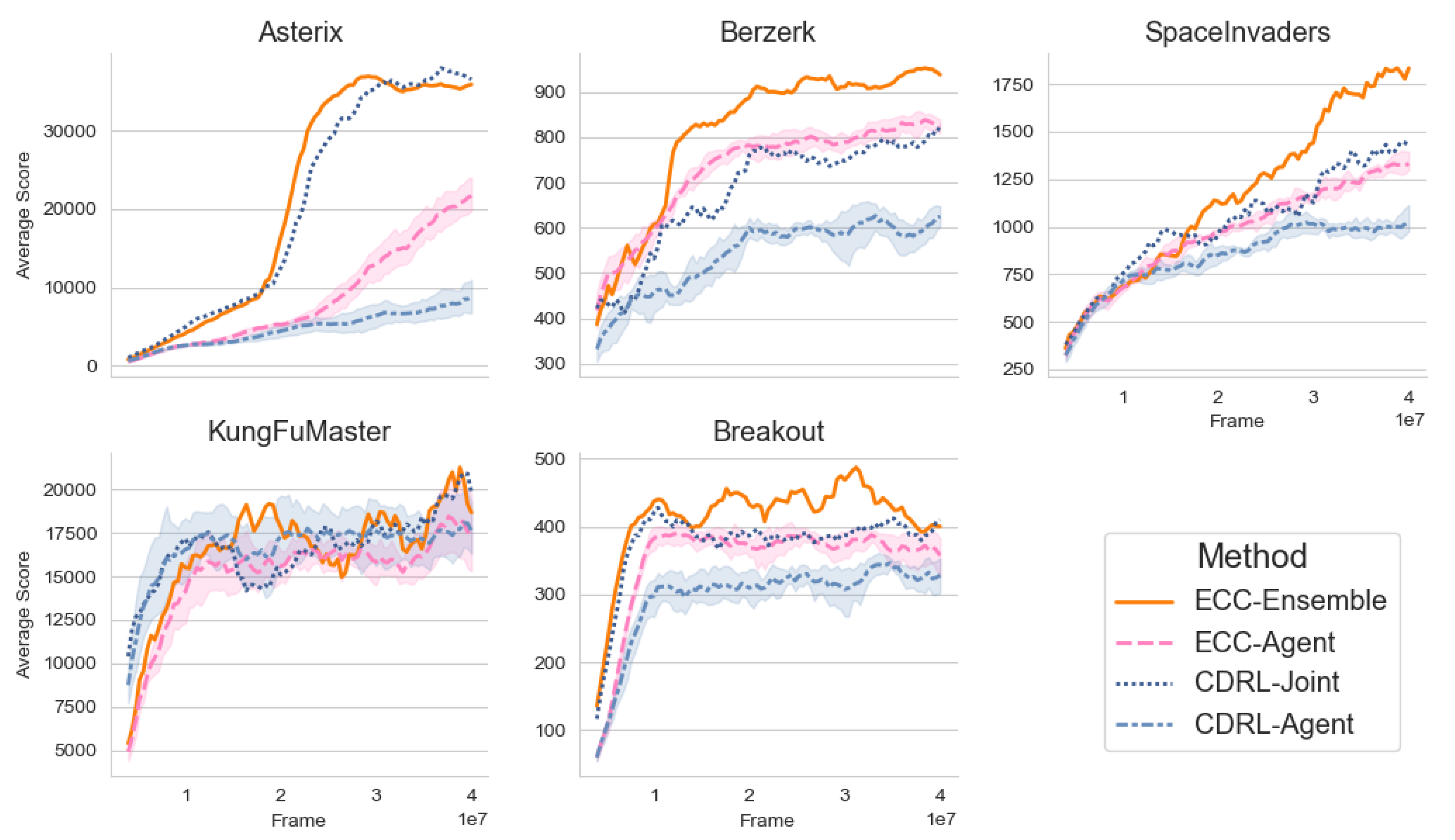
4.1. Online Performance

To get a sense of the algorithmic robustness and speed of learning, we report the online performance of agents and ensembles [7]. Under this protocol, we recorded the average return for each evaluation point during learning. We also stored the best average return score for all points of each seed.
We can see in Table 1 and Figure 2 that the extension ensemble was on par or outperformed the baseline in online performance over all five environments. Moreover, in four out of five games, single ECC agents had similar performance to the joint policy of k independently trained agents, which was the main training objective of the extension algorithm. We also note that in all environments, except possibly Breakout and KungFuMaster, ensemble agents seemed to be uncorrelated enough to generate a boost in performance by their joint information, while ECC agents had a better individual performance than single CDRL agents in four out of five games.

4.2. Relative Ensemble Sample Performance

Although ensembles will digest frames at nearly k times the rate of a single CDRL algorithm, we considered here the relative sample performance, where we looked at performance versus the total information accumulated by an algorithm. Under this protocol, we measured the relative ratio of mean evaluation scores as a function of the total amount of frames seen by each learning system. This would give us an idea of how efficiently an ensemble algorithm could translate experience into performance on a per-sample basis compared to single CDRL. Note that if single CDRL agents all converged to correlated errors, then the joint policy should eventually converge to 1 / k -efficiency in relative sample performance. Thus, in general, we should expect the relative performance to degrade as training progresses with diminishing ensemble benefits.
Table 2 shows the measured relative performance of the two ensemble methods, averaged over the first 40 M samples. We note that initial learning with ensembles may generate performance much higher than 1 / k -efficiency. We also note that the extension ensemble came close to full efficiency in Berzerk and Breakout, i.e., it displayed a near k-factor increase in learning rate. However, depending on the environment, the actual speed-up may vary wildly during learning, as shown in Figure 2.

5. Discussion

In this paper, we proposed and studied an extension of categorical distributional reinforcement learning, where we employed averaged learning targets over an ensemble. This extension implied an implicit sharing of information between agents during learning, where under the distributional paradigm, we should expect a richer and more robust set of predictions while preserving multimodality during aggregation. To test these assumptions, we did an initial empirical study on a subset of Atari 2600 games, where we employed essentially the same architecture and hyperparameter set as the C51 algorithm in [5]. In all cases, we saw that the single agent performance objective of the extension was accomplished. We also studied the effects of keeping extension amplified agents in an ensemble, where in some cases, the performance benefits were present and stronger than an averaged ensemble of independent agents.
We note that unlike massively distributed approaches such as Ape-X [26], the extension represents a decentralized distributed learning system with minimal overhead. As such, it naturally comes with poor scalability, but with greater efficiency on a per-sample basis. An interesting idea here would be to somewhat counteract the poor scalability by choosing agents with successively lower capacity as the ensemble size increases. We should then expect to see better performance with increasing size until a cutoff point is reached, hinting at the minimum capacity needed to find and represent strong solutions effectively.
We leave as future work the matter of convergence analysis and hyperparameter tuning, in particular the update period for a target ensemble network. It is quite possible that the update frequency of C51 was too aggressive when using ensemble targets. This may lead to premature convergence to correlated agents upon reaching difficult environmental plateaus with rarely seen transitions to more abundant rewards. Some interesting ideas here would be scheduled update periods or eventually switching to CDRL from a much stronger and robust level of individual performance. However, to gauge these matters fully, we would need a more comprehensive empirical study.   

Author Contributions

Conceptualization, B.L., J.N., and K.-O.L.; methodology, B.L. and J.N.; software, B.L.; validation, B.L.; formal analysis, B.L., J.N., and K.-O.L.; investigation, B.L.; data curation, B.L.; writing, original draft preparation, B.L.; writing, review and editing, B.L., J.N., and K.-O.L.; visualization, B.L.; supervision, K.-O.L.; project administration, K.-O.L. All authors read and agreed to the published version of the manuscript.

Funding

This research received no external funding.

Acknowledgments

The authors would like to thank the referees for comments that helped improve the presentation. The authors would also like to thank Morgan Ericsson, Department of Computer Science and Media Technology, Linnæus University, for productive discussions and technical assistance with the LNU-DISAHigh Performance Computing Platform.

Conflicts of Interest

The authors declare no conflict of interest.

Abbreviations

The following abbreviations are used in this manuscript:
CDRLCategorical Distributional Reinforcement Learning
MDPMarkov Decision Process
ECCEnsemble Categorical Control

Appendix A

Algorithm A1: Ensemble categorical control.
Input: Number of iteration steps N, ensemble size k, support z
  Initialize starting states x 1 , , x k in independent environments
  Initialize agent networks η θ 1 , , η θ k with random parameters θ 1 , , θ k
  Initialize target network η ¯ = 1 k i η θ i with θ i θ i
  Initialize replay buffers B 1 , , B k with the same size S
  for t = 1 N do
   for all i { 1 , , k } do
    Set a i to be a uniform random action with probability ε t
    Otherwise, set a i arg max a Q η θ i ( x i , a )
    Execute a i , and store the transition ( x i , a i , r i , x i ) in B i
    Set x i x i
   end for
   if t 0 mod P update then
    for all i { 1 , , k } do
     Initialize loss L 0
     Sample uniformly a minibatch B B i
     for all ( x , a , r , x ) B do
      Set a arg max a Q η ¯ ( x , a )
      Set L L + KL Π z f r # η ¯ ( x , a ) η θ i ( x , a )
     end for
     Update θ i by a gradient descent step on L
    end for
   end if
   if t 0 mod P clone then
    for all i { 1 , , k } do
     Update target network with θ i θ i
    end for
   end if
  end for

References

  1. Singh, S.P. The efficient learning of multiple task sequences. In Advances in Neural Information Processing Systems; MIT Press: Cambridge, MA, USA, 1992; pp. 251–258. [Google Scholar]
  2. Sun, R.; Peterson, T. Multi-agent reinforcement learning: weighting and partitioning. Neural Netw. 1999, 12, 727–753. [Google Scholar] [CrossRef]
  3. Wiering, M.A.; Van Hasselt, H. Ensemble algorithms in reinforcement learning. IEEE Trans. Syst. Man, Cybern. Part B (Cybernetics) 2008, 38, 930–936. [Google Scholar] [CrossRef] [PubMed] [Green Version]
  4. Faußer, S.; Schwenker, F. Selective neural network ensembles in reinforcement learning: Taking the advantage of many agents. Neurocomputing 2015, 169, 350–357. [Google Scholar] [CrossRef]
  5. Bellemare, M.G.; Dabney, W.; Munos, R. A distributional perspective on reinforcement learning. In Proceedings of the 34th International Conference on Machine Learning, Sydney, Australia, 6–11 August 2017; Volume 70, pp. 449–458. [Google Scholar]
  6. Morimura, T.; Sugiyama, M.; Kashima, H.; Hachiya, H.; Tanaka, T. Parametric return density estimation for reinforcement learning. In Proceedings of the Twenty-Sixth Conference on Uncertainty in Artificial Intelligence, Catalina Island, CA, USA, 8–11 July 2010; pp. 368–375. [Google Scholar]
  7. Dabney, W.; Rowland, M.; Bellemare, M.G.; Munos, R. Distributional reinforcement learning with quantile regression. In Proceedings of the Thirty-Second AAAI Conference on Artificial Intelligence, New Orleans, LA, USA, 2–7 February 2018. [Google Scholar]
  8. Dabney, W.; Ostrovski, G.; Silver, D.; Munos, R. Implicit Quantile Networks for Distributional Reinforcement Learning. Int. Conf. Mach. Learn. 2018, 80, 1096–1105. [Google Scholar]
  9. Lyle, C.; Bellemare, M.G.; Castro, P.S. A comparative analysis of expected and distributional reinforcement learning. In Proceedings of the AAAI Conference on Artificial Intelligence, Honolulu, HI, USA, 27 January–1 February 2019; Volume 33, pp. 4504–4511. [Google Scholar]
  10. Rowland, M.; Bellemare, M.; Dabney, W.; Munos, R.; Teh, Y.W. An Analysis of Categorical Distributional Reinforcement Learning. In Proceedings of the International Conference on Artificial Intelligence and Statistics, Canary Islands, Spain, 9–11 April 2018; pp. 29–37. [Google Scholar]
  11. Bellemare, M.G.; Le Roux, N.; Castro, P.S.; Moitra, S. Distributional reinforcement learning with linear function approximation. In Proceedings of the 22nd International Conference on Artificial Intelligence and Statistics, Okinawa, Japan, 16–18 April 2019; pp. 2203–2211. [Google Scholar]
  12. Bellemare, M.G.; Naddaf, Y.; Veness, J.; Bowling, M. The Arcade Learning Environment: An Evaluation Platform for General Agents. J. Artif. Intell. Res. 2013, 47, 253–279. [Google Scholar] [CrossRef]
  13. Rizzo, M.L.; Székely, G.J. Energy distance. Wiley Interdiscip. Rev. Comput. Stat. 2016, 8, 27–38. [Google Scholar] [CrossRef]
  14. Bertsekas, D.P.; Tsitsiklis, J.N. Neuro-Dynamic Programming; Athena Scientific: Belmont, MA, USA, 1996. [Google Scholar]
  15. Villani, C. Optimal Transport: Old and New; Springer Science & Business Media: Berlin, Germany, 2008; Volume 338. [Google Scholar]
  16. Bellemare, M.G.; Danihelka, I.; Dabney, W.; Mohamed, S.; Lakshminarayanan, B.; Hoyer, S.; Munos, R. The Cramer Distance as a Solution to Biased Wasserstein Gradients. arXiv 2017, arXiv:1705.10743. [Google Scholar]
  17. Mnih, V.; Kavukcuoglu, K.; Silver, D.; Rusu, A.A.; Veness, J.; Bellemare, M.G.; Graves, A.; Riedmiller, M.; Fidjeland, A.K.; Ostrovski, G.; et al. Human-level control through deep reinforcement learning. Nature 2015, 518, 529–533. [Google Scholar] [CrossRef] [PubMed]
  18. Breiman, L. Bagging predictors. Mach. Learn. 1996, 24, 123–140. [Google Scholar] [CrossRef] [Green Version]
  19. Goodfellow, I.; Bengio, Y.; Courville, A. Deep Learning; MIT Press: Cambridge, MA, USA, 2016. [Google Scholar]
  20. Brockman, G.; Cheung, V.; Pettersson, L.; Schneider, J.; Schulman, J.; Tang, J.; Zaremba, W. OpenAI Gym. arXiv 2016, arXiv:1606.01540. [Google Scholar]
  21. Clemen, R.T.; Winkler, R.L. Combining probability distributions from experts in risk analysis. Risk Anal. 1999, 19, 187–203. [Google Scholar] [CrossRef]
  22. Casarin, R.; Mantoan, G.; Ravazzolo, F. Bayesian calibration of generalized pools of predictive distributions. Econometrics 2016, 4, 17. [Google Scholar] [CrossRef] [Green Version]
  23. Johnson, R.A.; Wichern, D.V. Applied Multivariate Statistical Analysis; Pearson: Harlow, UK, 2014. [Google Scholar]
  24. Lindenberg, B.; Nordqvist, J.; Lindahl, K.O. bjliaa/ecc: ecc; (Version v0.3-alpha). Zenodo: 2020. Available online: https://zenodo.org/record/3760246#.XrP1Oi4za1U (accessed on 22 April 2020).
  25. Hill, A.; Raffin, A.; Ernestus, M.; Gleave, A.; Kanervisto, A.; Traore, R.; Dhariwal, P.; Hesse, C.; Klimov, O.; Nichol, A.; et al. Stable Baselines. 2018. Available online: https://github.com/hill-a/stable-baselines (accessed on 22 April 2020).
  26. Horgan, D.; Quan, J.; Budden, D.; Barth-Maron, G.; Hessel, M.; van Hasselt, H.; Silver, D. Distributed Prioritized Experience Replay. arXiv 2018, arXiv:1803.00933. [Google Scholar]
Figure 1. Low capacity CDRL implementations in the LunarLander-v2 environment. We can see that the enhanced performance of an average joint policy of five agents may not vanish due to agents settling on distinct sub-optimal policies.
Algorithms 13 00118 g001
Figure 2. Online performance over the first 40 M frames. The evaluation scores shown are moving averages over 4 M frames. The data are available at [24].
Algorithms 13 00118 g002
Table 1. Best achieved evaluation scores in online performance over the first 40 M samples, here with 95% confidence when there is more than one seed. The data are available at [24].
GameCDRL AgentECCAgentCDRL JointECCEnsemble
Asterix12,998 ± 304228,196 ± 90339,41338,938
Berzerk795 ± 47958 ± 128901034
SpaceInvaders1429 ± 911812 ± 8718502395
Breakout444 ± 44546 ± 27515665
KungFuMaster27,984 ± 176727,302 ± 221325,82629,629
Table 2. Rough estimates of relative sample performance, here expressed as percentages of CDRL agent performance and averaged over the first 40 M samples. The data are available at [24].
MethodAsterixBerzerkBreakoutSpaceInvadersKungFuMaster
ECCEnsemble47.7 %93.7 %93.7 %63.4 %66.9 %
CDRL Joint56.3 %86.7 %86.1 %67.2 %87.0 %

