Abstract
The electricity market is a complex, evolutionary, and dynamic environment. Forecasting electricity prices is an important issue for all electricity market participants. In this study, we shed light on how to improve electricity price forecasting accuracy through the use of a machine learning technique—namely, a novel genetic programming approach. Drawing on empirical data from the largest EU energy markets, we propose a forecasting model that considers variables related to weather conditions, oil prices, and CO2 coupons and predicts energy prices 24 h ahead. We show that the proposed model provides more accurate predictions of future electricity prices than existing prediction methods. Our important findings will assist the electricity market participants in forecasting future price movements.
1. Introduction
The energy sector has suffered significant restructuring that has increased the complexity of the electricity markets [1]. In Europe, as well as in other countries worldwide, the electricity market’s deregulation has led to new competitive positions among its participants, namely generators, distributors, and consumers, as well as insecurity about the future evolution of electricity markets [2].
An essential characteristic of electricity markets is their pricing mechanisms, which can affect the competition, efficiency, consumers, and revenue of the participating players [3]. Accuracy in forecasting electricity prices reduces the risk of under/overestimating the revenue for the participants and provides better risk management [4].
In the present deregulated scenario, electricity price forecasting has emerged as one of the major research fields within the energy sector [5,6]. The field of electricity price forecasting, similar to financial forecasting in stock market movements [7], is characterized by intensive data, noise, non-stationarity, a high degree of uncertainty, and hidden relationships. Many factors interact in the electricity sector, including political events, general economic conditions, and traders’ expectations [6]. Therefore, predicting electricity market price movements is quite challenging [8].
Scholars are actively engaged in developing tools and algorithms for price and load forecasting [9,10]; while load forecasting has reached advanced stages of development, price forecasting techniques are still in their early stages of maturity [5]. Aggarwal, Saini [5] provide a comprehensive review of the main methodologies used in electricity price forecasting and a detailed analysis of extant studies based on the time horizon for prediction, the input and output variables used, the obtained results, the data points used for analysis, and the preprocessing technique/model architecture employed.
While prior studies primarily focus on spot [11,12,13,14] or day-ahead [15,16,17,18,19] electricity price forecasting, little research addresses the long-term forecasting horizon [20,21] or even moving between short-term and long-term horizons [22].
The current flood of data on the various attributes affecting electricity pricing makes traditional data analysis methods (i.e., the bulk of activities involved in generating queries and reports on what electricity prices have been in the past) seem quaint and unfeasible for understanding today’s pricing complexity. Forecasting near-future energy pricing considers, but is not limited to, the historical prices of gasoline, crude oil, and electricity, along with predicted weather patterns, locations, extreme weather events, the discovery of new fuel reserves, and increased energy demands. If we want to respond to the almost infinite number of variations in electricity pricing attributes, we need a different approach.
When simple data analysis methods cannot do the job, we must adopt more autonomous methods that automatically employ alternative variables in combination to create multiple models with an optimized fit to the data. Extant studies introduce various models that describe (spot, day-ahead, and near-future) price behavior in power markets (see [23]) by considering a (limited) number of variables. This paper develops a model for forecasting future electricity prices using a novel genetic programming approach. Drawing on empirical data about weather conditions, oil prices, and CO2 coupons from the largest EU energy market, we show that the proposed model provides more accurate predictions of future electricity prices compared to extant prediction methods.
The paper unfolds as follows. In the next section, we present the challenges of electricity price forecasting. We then introduce the novel genetic programming approach as a way to tackle the present challenges. Next, we develop our prediction model and apply it to predict the energy prices 24 h ahead. Finally, we discuss our proposed model, highlighting our contributions to the field and offering future research directions.
2. Challenges of Electricity Price Forecasting
Since the deregulation in electricity markets, price forecasting has become an extremely valuable tool. Electricity market participants make extensive use of price prediction techniques; an accurate price forecast for an electricity market has a decisive impact on the bidding strategies by producers or consumers and on the price negotiations of a bilateral contract. In both pool markets and bilateral contracts, predicting next-day electricity prices or prices for the next several months (or even years) is of the foremost importance to allow electric companies to adjust their daily bids or monthly/yearly schedules for contracts. As energy service companies buy electricity from the pool and from bilateral contracts to sell it to their clients, they seek good short-term and long-term price forecast information to maximize their own benefits [3].
As Hong, Pinson [24] argues, electricity prices, and particularly price spikes, are influenced heavily by a wide range of factors (e.g., transmission congestion, generation outages, and market participant behaviors) other than the electricity demand. These factors, their hidden relationships, and the uncertainties associated with them are difficult to incorporate into electricity price forecasting models.
Artificial intelligence-based electricity price forecasting methods have been recently proposed to counter the above-mentioned problems [18,21,25]. The main reasoning for employing these methods is their ability to infer hidden relationships in data. However, many of these methods still have along several shortcomings that limit the extent of their exploitation [3]. These deficiencies include high prediction errors for price forecasting, the inability to effectively exploit local data characteristics or capture global data trends, and the excessive computational requirements for price prediction. Overall, despite the current efforts, significant errors remain in price predictions, confirming the need for more efficient forecast methods in this field [6].
To answer this call, this work proposes a machine learning system based on a recently defined variant of genetic programming, a machine learning technique that has demonstrated its ability to produce human-competitive results [26]. In particular, as discussed in the following section, the proposed system provides energy market participants a viable option for addressing the energy price forecasting task considering a 24 hour prediction horizon, thereby overcoming the main limitations of existing methods.
Among the vast amount of existing machine learning techniques that are presently available, this study focuses on genetic programming for several reasons. First of all, there is increasing interest in the scientific literature concerning the interpretability of artificial intelligence (AI) models [27]. This interest ranges from the business domain [28] to the health-care sector [29]. Moreover, AI has been identified to potentially offer significant benefits to a large range of domains, including the energy market [30]. The growing interest in this topic is accompanied by the popularity of AI-based models: Despite their ability to produce human-competitive results in an increasing number of complex tasks, these models are essentially black boxes, as no information is provided about how they achieved their predictions. In other words, as a final AI user, we know the prediction that a given AI model produced, but we do not know why this particular prediction was made. This could be an important limitation to the more wide-scale adoption of AI, as users show more willingness to use a particular model when they can understand why particular decisions are being made [31]. In the context of the applicative domain considered in this project, the possibility of obtaining explainable models could allow us to make better-informed decisions on how operate in the energy market. Additionally, at the European level, the importance of developing an explainable AI is also motivated by the recent introduction of the General Data Protection Regulation, which forbids the use of solely automated decisions. In the US, the Defense Advanced Research Projects Agency (DARPA) noted that explainable AI will be essential if users are to understand, appropriately trust, and effectively manage this incoming generation of artificially intelligent partners [32].
The ability to interpret the final model is a characteristic that distinguishes genetic programming from other machine learning techniques [33], such as neural networks, support vector machines, or K-nearest neighbors. Additionally, genetic programming can perform automatic feature selection, thus allowing the domain expert to gain a clear understanding about the most relevant variables for the problem under analysis.
All of these properties make genetic programming a suitable machine learning technique for addressing the energy price forecasting problem.
3. Method
Genetic programming (GP) [34] is a method that belongs to the computational intelligence research area called evolutionary computation. GP consists of the automated learning of computer programs by means of a process inspired by Darwin’s theory of biological evolution. In the context of GP, the word program can be interpreted in general terms. Thus, GP can be applied, for instance, to learning expressions, functions and, as in this work, data-driven predictive models. Crucial to GP are the definitions of the representations used to encode the programs and the function used to quantify the program’s quality, called an objective function or fitness.
Starting from an initial population of programs, which are typically generated at random, the objective of GP is to navigate the space of all programs that can be represented with predefined encoding, searching for the most appropriate programs to solve the problem at hand. Generation by generation, GP stochastically transforms (by means of genetic operators) the populations of programs into new populations of possibly more applicable programs. Several different representations exist, but the one most commonly used encodes a solution as a LISP-like tree [34].
Despite its success in solving complex real-world problems [26], traditional syntax-based genetic operators produce new individuals by operating a blind transformation of the parents. In more detail, knowing the output produced by the parent individuals for a set of training observations does not provide useful information on the output that the children will produce. In other words, traditional mutation and crossover operators directly work on the structure of the individuals without considering any information associated with their behavior or, as commonly found in the literature [35], semantics.
This fact is counter-intuitive because, from the point of view of the GP practitioner, what matters is the output produced by the individuals on a set of observations. On the other hand, the structure of the solution (i.e., how the solution is represented) generally plays a secondary role. For this reason, recent years have seen rising interest in the definition of genetic operators able to directly act at the semantic level [35].
Among the different semantic methods, the work proposed by Moraglio, Krawiec [36] made a fundamental contribution to this field, providing the definition of genetic operators (called geometric semantic operators) that, unlike other existing approaches, are able to directly include the concept of semantics in the search process.
Geometric semantic operators (GSOs) have proved their suitability for solving real-world problems [35,37] and have achieved better performance in standard syntax based GP. This competitive advantage is related to the fact that GSOs induce a unimodal fitness landscape on any problem consisting of matching sets of input data into known targets (e.g., supervised learning problems such as regression and classification). According to the theory of fitness landscapes [38], this process improves the ability of GP to find optimal (or near-optimal) solutions.
The definitions of semantic crossover and semantic mutation for regression problems is given as follows:
Geometric Semantic Crossover (GSC) Moraglio, Krawiec [36]. Given two parent functions T1, T2: Rn → R, the geometric semantic crossover returns the real function TXO = (T1 · TR) + ((1 − TR) · T2), where TR is a random function such that TR: Rn → [0; 1].
To constrain TR when producing values in [0; 1], we make use of the sigmoid function TR = 1 / (1 + e-Trand), where Trand is a random tree with no constraints on the output values.
Geometric Semantic Mutation (GSM) Moraglio, Krawiec [36]. Given a parent function T: Rn → R, the geometric semantic mutation with mutation step ms returns the real function TM = T + ms · (TR1 − TR2), where TR1 and TR2 are random real functions. Henceforth, we refer to the GP algorithm that uses GSOs as Geometric Semantic Genetic Programming (GSGP).
Despite the success of GSGP, an important limitation prevents the use of GSOs in applications where it is important to have a reliable model in a limited amount of time. As shown in different studies [37,39], GSOs require a large number of iterations before converging towards an optimal solution. On the other hand, considering the application presented in this paper, it is fundamental for an energy market participant to know the predicted price of the energy as soon as possible in such a way that he or she can safely operate over different trading terms.
In this study we propose a system that combines GSGP with a local search optimizer, as described by Castelli, Trujillo [40]. The idea of combining a local searcher with more exploratory techniques comes from the analysis of evolutionary computation techniques, whose behavior is determined by the exploitation and exploration relationship kept throughout the run [41]. Thus, there is the need for hybrid evolutionary approaches whose main task is to optimize the performance of the direct evolutionary approach (GSGP in this paper). In particular, the hybridization between evolutionary algorithms and local search produces memetic algorithms. Memetic algorithms are orders of magnitude faster and more accurate than evolutionary algorithms for different classes of problems [41]. Despite the potential advantages of these hybrid methods, the use of local searches within geometric semantic genetic programming was fully studied only in a recent contribution [42].
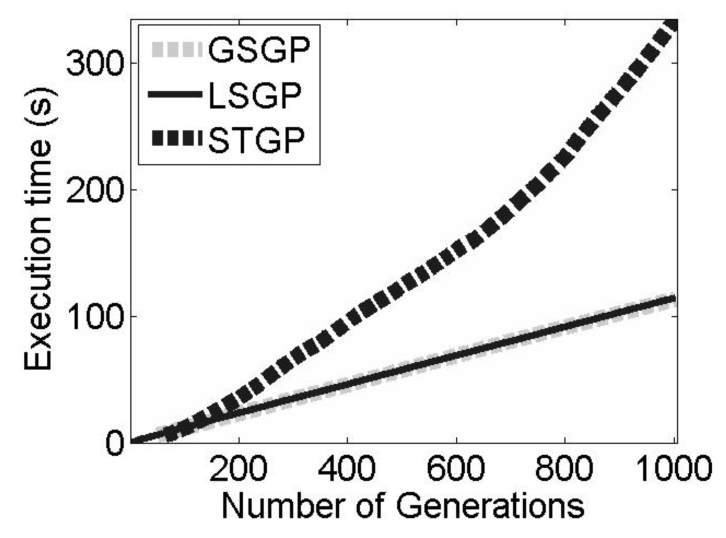
In the context of this work, the use of a local searcher is motivated by the improvement of the convergence speed of GSGP when finding good quality solutions. In this work, we include a local searcher (LS) within the GSM mutation operator. While this is not the only viable option, it is the one that does not produce a significantly negative effect on the execution time of the system. To observe this fact, it is possible to consider (Figure 1) the execution time of standard GP, GSGP, and the proposed system (LSGP) for completing a GP run with 1000 iterations (generations). The running times of GSGP and LSGP are comparable but, as discussed in the following section, LSGP is able to achieve the same accuracy as GSGP by considering only a few iterations.
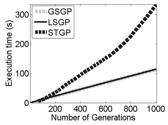
Figure 1.
Comparison between the execution time of different GP systems. GSGP stands for Geometric Semantic Genetic Programming, the GP system that uses the GSC and GSM operators; LSGP is the GSGP version in which the GSM operator is combined with the local search operator; STGP refers to the traditional GP algorithm that makes use of standard syntax-based genetic operators.
The GSM with LS (LSGSM) is defined as follows: Given an individual T, the LSGSM operator produces a new individual such that , where ; here, replaces the mutation step parameter ms used in the definition of GSM.
This formulation defines a basic multivariate linear regression problem that can be solved, for example, by Ordinary Least Square regression (OLS). Hence, after the application of geometric semantic mutation, OLS is applied to the previous expression to obtain the values of the parameters () that best fit the training instances. As explained by Castelli, Trujillo [40], combining the exploration ability of GSGP with the exploitation ability of a local search method allows LSGP to find good quality solutions in a small number of generations while also avoiding the excessive specialization of a model of the training instances and, consequently, overfitting.
Thanks to its properties, LSGP provides an efficient tool to energy market participants for the energy price forecasting task. As demonstrated in the experimental phase, this system is able to outperform existing machine learning techniques, providing an accurate prediction of the energy price in a negligible amount of time. The system that implements the geometric semantic operators used in this work is available at the following URL: http://gsgp.sourceforge.net/. The system was implemented in C++. The computational cost of evolving a population of n individuals for g generations is O(ng), while the cost of evaluating a new unseen instance is O(g) [43,44].
The LSGP algorithm is reported in Algorithm 1.
| Algorithm 1: The GP algorithm. |
| 1: Population ß InitializePopulation(population_size, problem_variables) |
| 2: EvaluatePopulation(Population) |
| 3: S_best ß GetBestSolution(Population) |
| 4: num_iterations ß 0 |
| 5: While (num_iteration < num_generations) |
| 6: Children_pop ß Ø |
| 7: Children_pop ß Children_pop U S_best |
| 8: While (Size(Children_pop) < population_size) |
| 9: Operator ß SelectGeneticOperator(Crossover_Rate, Mutation_Rate) |
| 10: If (Operator == CrossoverOperator) |
| 11: Parent_1 ß SelectParent(Population) |
| 12: Parent_2 ß SelectParent(Population) |
| 13: Child = GSC(Parent_1,Parent_2) |
| 14: Children_pop = Children_pop U Child |
| 15: ElseIf (Operator == MutationOperator) |
| 16: Parent_1 ß SelectParent(Population) |
| 17: Child = LSGSM(Parent_1) |
| 18: Children_pop = Children_pop U child |
| 19: Else |
| 20: Parent_1 ß SelectParent(Population) |
| 21: Children_pop = Children_pop U parent_1 |
| 22: End |
| 23: End |
| 24: EvaluatePopulation(Children_pop) |
| 25: S_bset ß GetBestSolution(Children_pop) |
| 27: Population ß Children_pop |
| 28: num_iteration ß num_iteration + 1 |
| 29: End |
| 30: Return (S_best) |
4. Experimental Phase
This section presents the experimental settings and the performance achieved with the proposed system. In particular, the first part of the experimental phase is dedicated to a comparison between GSGP and LSGP to assess whether the inclusion of a local searcher is beneficial for the problem at hand. Then, in a subsequent phase, LSGP is compared against traditional statistical and machine learning techniques that are commonly used to address forecasting problems. In the first part of the experimental phase, standard GP was not considered because of its unbearable running time and because it performs poorly with respect to GSGP in this kind of forecasting application [39,40].
4.1. Data
Extant studies [43,44,45,46] indicate that electricity prices have time-varying behavior, with periods of longer mean reversion during which there may be stronger associations with fuel and carbon prices. On the other hand, the different meteorological variables are not widely investigated. Most of the proposed models employ temperature and wind as the key meteorological variables [8,47,48].
The considered dataset consists of 15 variables, ranging from alternative energy sources to weather conditions. In our analysis, we considered the data from 1 January 2010 through 30 June 2015 for all model variables. Each observation represents one day, and the prediction horizon is 24 h. As an alternative energy source (variable X0), the crude oil spot price in USD per barrel for EU was used [49]. Apart from alternative energy sources, the EEX EU Emission Allowances have also been taken into consideration (variable X1) as the spot EU emissions allowance in price per EUR/tCO2 [50]. Variables X2 through X15 relate to the weather conditions and include air temperature, air density, ground temperature, air pressure, relative humidity, wind speed, maximum intraday air temperature, minimum intraday air temperature, minimum intraday air temperature at ground level, maximum intraday wind speed, next-day precipitation of rain to cover a horizontal ground surface, next day precipitation of snow to cover a horizontal ground surface, sunshine duration, and snow depth. The data for the weather conditions in Munich, Germany were obtained from the online data source “Deutscher Wetterdienst” [51]. All the variables were normalized and are dimensionless. Thus, it is possible to combine all variables without considering their different units of measurement. Table 1 provides a list of all variables used in this study.

Table 1.
Model variables available in the considered dataset. Observations collected on a daily basis; the task is to predict the target variable in the next 24 h.
4.2. Experimental Settings and Results for GP-Based Systems
This section reports the experimental settings considered for evaluating the performance of the considered GP-based systems. We tested the proposed LSGP against GSGP. A total of 100 runs were performed with each technique. This is a fundamental aspect given the stochastic nature of the considered systems. In each run, we used data until 2013 for training purposes, while the remaining data (until 2015) were used to assess the performance of the systems on unseen data (i.e., the generalization ability of the solutions). All the runs used populations of 200 individuals, and the evolution stopped after 300 generations. Tree initialization was performed using the Ramped Half-and-Half method [34] with a maximum initial depth equal to 6. The function set contained the arithmetic operators +, −, *, and protected division [34]. The terminal set contained 16 variables, each corresponding to a different feature in the dataset.
Mutation was used with a probability of 0.6. For GSM, a random mutation step was considered in each mutation event. The crossover rate was 0.4. Survival from one generation to the other was always guaranteed for the best individual of the population (elitism). These values were selected after a preliminary tuning phase that was performed through a grid-search to find the ideal values of these parameters.
In particular, the training set was split into five folds, with the first four folds used to train the model, and the fifth fold used to assess the performance of the model on unseen data.
At the end of this procedure, we trained the model with the whole training set, taking into account the values of the parameters resulting in the best performance on the validation fold.
We tested the following parameters: for the mutation rate, values from 0.1 to 0.8 with a step of 0.05 were considered; for the crossover rate, values from 0.1 to 0.8 with a step of 0.05 were taken into account; for the number of generations, we considered the values of 100, 300, and 500; for the population size, values of 50, 100, 200, 300, and 500 were considered.
The performance, across the different configurations, is stable, and increasing the number of generations and the population size beyond the considered values provided no significant improvements in performance.
Fitness was calculated by using the Mean Absolute Error (MAE) between the predicted and target values. The definition of this error measurement is the following:
where is the output of a GP individual on the i-th training case, and is the target value for that training case. N denotes the number of samples in the training or testing subset, and Q contains the indices of that set.
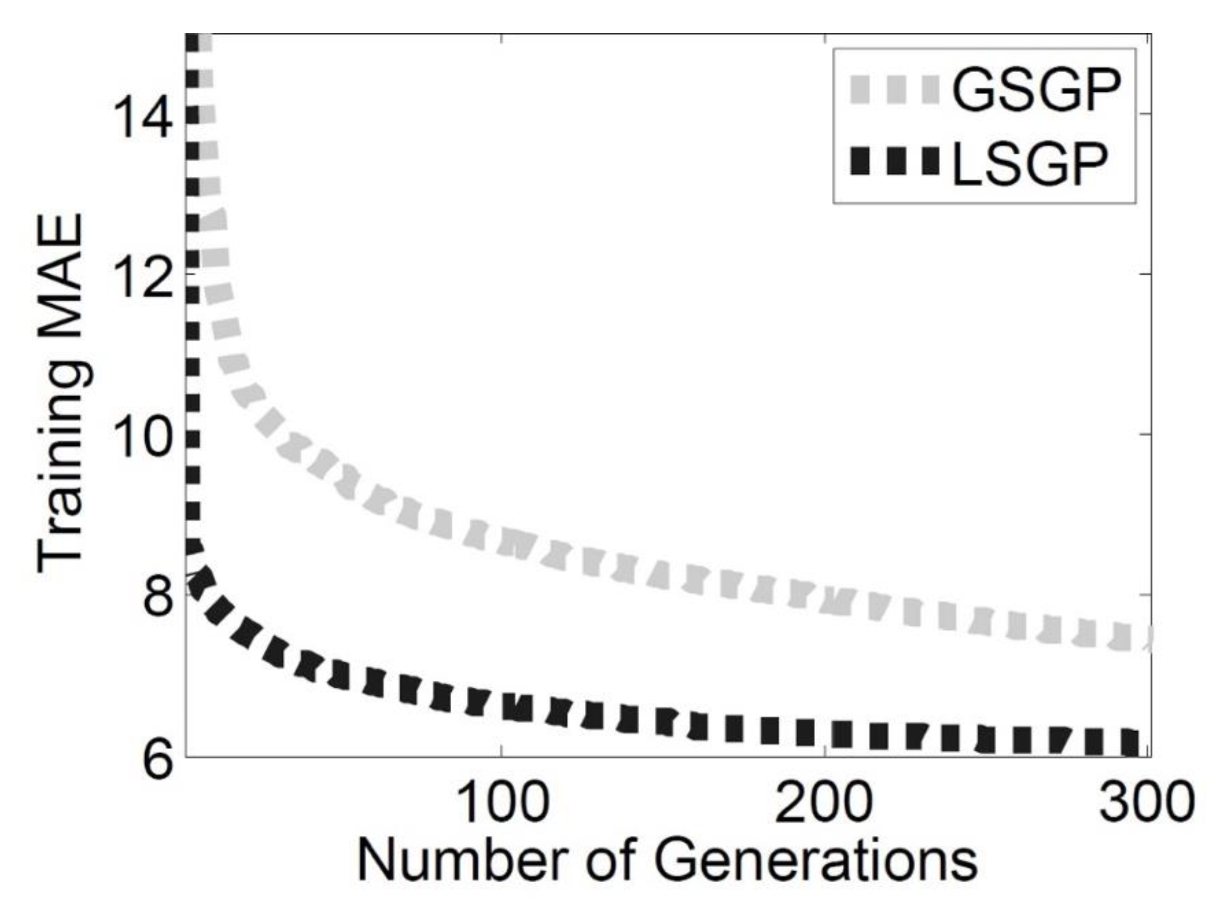
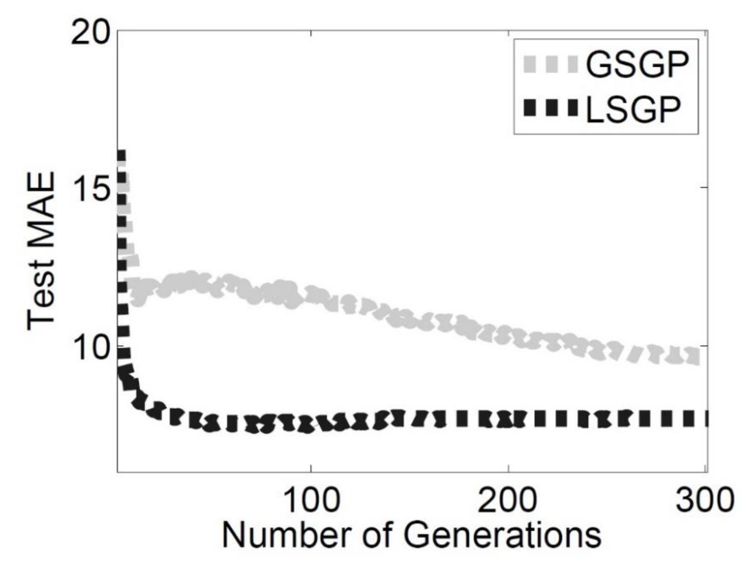
The results of this first part of the experimental phase are reported in Figure 2 and Figure 3 using the curves of the training and test MAE.
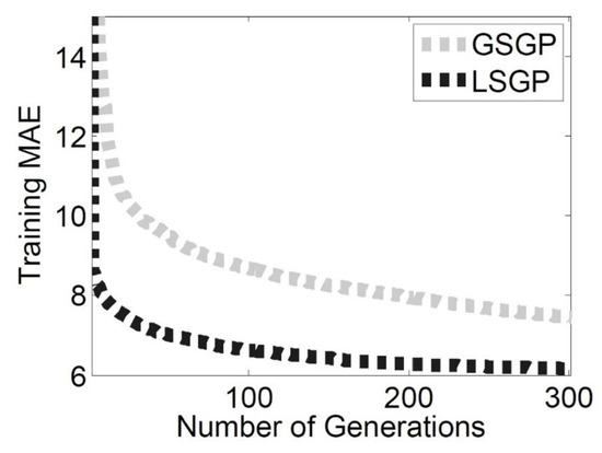
Figure 2.
Training Mean Absolute Error (MAE). The plots show the median over 100 runs. The training MAE is expressed in Euros. The light gray line represents Geometric Semantic Genetic Programming, while the black line represents Geometric Semantic Genetic Programming with Local Search.
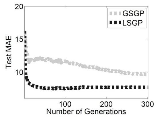
Figure 3.
Test MAE. The plots show the median over 100 runs. The Test MAE is expressed in Euros. The light gray line represents Geometric Semantic Genetic Programming, while the black line represents Geometric Semantic Genetic Programming with Local Search.
Considering the results on the training set (Figure 2), the LSGP outperforms GSGP. In particular, the inclusion of a local searcher in the GSM operator allows the GP process to converge into a smaller number of generations with respect to GSGP, for which the GSM operator without a local searcher is used. This observable increase in speed allows LSGP to achieve the same good quality solutions after 20 generations obtained by GSGP at the end of the search process, thereby saving the computational effort needed to build the model. Considering the fitness values achieved at the end of the search process, the difference between the two systems taken into account is still notable.
Similar considerations can be drawn when the fitness of the test instances (Figure 3) is taken into account. LSGP is able to outperform GSGP and, even more importantly, the solutions produced by LSGP do not overfit the training instances. Hence, LSGP is able to produce good quality solutions that are also able to generalize unseen test cases. This is an important property in a real and dynamic application like the one we are considering.
To assess the statistical significance of these results, a set of statistical tests was performed on the median errors. Preliminary analysis using the Lilliefors test (with α = 0.05) showed that the data were not normally distributed. Thus, a rank-based statistic was used. The Mann–Whitney rank-sum test for pairwise data comparison was used with the alternative hypothesis that the samples do not have equal medians. The p-values returned by the test (3.018 × 10⁻¹¹ for the training MAE and 8.6632 × 10⁻⁷ for the test MAE) confirm that LSGS is able to outperform GSGP by producing solutions with a significantly smaller MAE than the latter system.
To perform a fair comparison between the two systems, it is also important to consider the computational time required to solve the linear regression problem posed by LSGSM. For this reason, Table 2 reports the median running time (as well as the standard deviation), expressed in seconds, of the same 100 runs discussed above. The extra computational effort required by LSGSM is negligible, and a subsequent statistical validation confirmed that the difference between the running times of the two systems is not statistically significant.

Table 2.
Median and standard deviation of the running time (in seconds) for the two GP based systems.
4.3. Comparison with Other State-of-the-Art Machine Learning Techniques
In the second part of the experimental phase, the performance of LSGP was compared to that achieved with the other machine learning and statistical techniques commonly used to address forecasting problems. The objective of this section is to assess if, besides outperforming GSGP, LSGP is able to produce better models with respect to the other techniques considered.
The techniques considered to perform this comparison are the following: linear regression (LIN) [52], ordinary least square regression (SQ) [53], isotonic regression (ISO) [54], radial basis function network (RBF) [55], multilayer perceptron trained with backpropagation (NN) [55], and support vector machine (SVM) [56] with a polynomial kernel.
The implementation provided by the WEKA machine learning software [57] was used in this experimental phase. A tuning phase was performed with the objective of finding suitable values for the parameters that characterize the techniques considered. The tuning phase was performed by using the grid search functionality provided by Weka, which allows searching for the best parameters’ values.
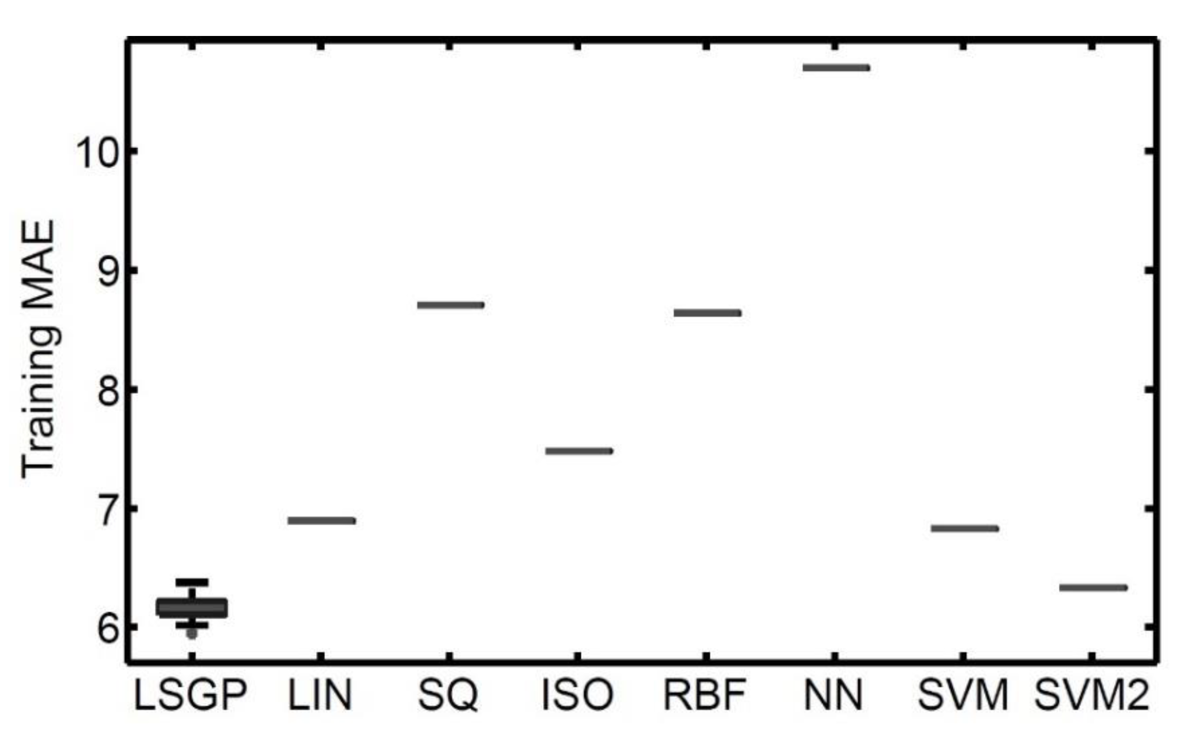
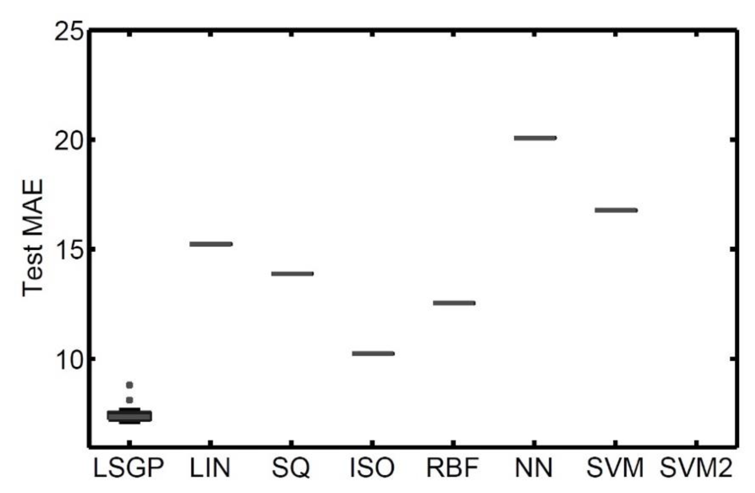
The boxplots reported in Figure 4 and Figure 5 show a comparison between the performance achieved by using the different machine learning techniques considered. On each box, the central mark is the median, the edges of the box are the 25th and 75th percentiles, and the whiskers extend to the most extreme data points not considered outliers. In the boxplots, SVM refers to support vector machines with a polynomial kernel of degree 1, while SVM-2 refers to support machines with a polynomial kernel of the second degree.

Figure 4.
Boxplots of the training MAE calculated over 100 runs. On each box, the central mark is the median, the edges of the box are the 25th and 75th percentiles, and the whiskers extend to the most extreme data points not considered outliers. The MAE is expressed in Euros. LIN stands for linear regression, SQ stands for ordinary least square regression, ISO stands for isotonic regression, RBF stands for radial basis function network, NN stands for multilayer perceptron trained with backpropagation, and SVM stands for support vector machine with a polynomial kernel (of second degree for SVM2).
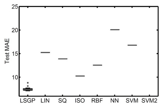
Figure 5.
Boxplots of the test MAE calculated over 100 runs. On each box, the central mark is the median, the edges of the box are the 25th and 75th percentiles, and the whiskers extend to the most extreme data points not considered outliers. The MAE is expressed in Euros. LIN stands for linear regression, SQ stands for ordinary least square regression, ISO stands for isotonic regression, RBF stands for radial basis function network, NN stands for multilayer perceptron trained with backpropagation, and SVM stands for support vector machine with a polynomial kernel (of second degree for SVM2).
Considering the MAE on the training instances, the LSGP is observably the best performer, with MAE values that are comparable to the ones achieved with SVM-2. The worst technique on the training set is the multilayer perceptron, followed by SQ and RBF. ISO, LIN, and SVM produce results that are better than the latter techniques but still worse than the results achieved with LSGP. To summarize the results observed with the training set, LSGP is the best performer, and, among the other techniques taken into account, SVM-2 is able to produce comparable good quality solutions.
While the results obtained from a training set give a good indication of the suitability of a given technique to match the training data, it is more important to assess if a given technique can produce the same positive results on unseen test cases. This will give an indication of the generalization ability of the model returned by the technique. Indeed, a model that perfectly matches the training set but cannot properly handle unseen test cases is completely useless in real applications. Figure 5 shows the performance achieved by the machine learning techniques considered for the test set. The first observation is that LSGP is still the best performer and can also produce good quality results with the test set. On the other hand, SVM-2 is now the worst technique, thereby showing the method’s poor generalization ability: SVM-2 is not able to achieve the same good quality results for the test set that were found for the training instances. The same observation applies to LIN and SVM. While they can produce satisfactory results with the training set, they cannot show the same performance for the test set. For the training set, the worst technique with the test set is multilayer perceptron (NN).
According to the results obtained from the experimental phase, it is possible to draw some interesting considerations with respect to the stability of the techniques taken into account. In particular, focusing on the differences between the training and test MAE and LSGP can provide robust models that are able to translate the excellent performance achieved for the training set to the test set. Linear regression and ordinary least square regression are characterized by some amount of overfitting, and it seems that they learned patterns from the training set that are not useful for generalization with unseen data. This issue is even more evident when considering artificial neural networks and support vector machines. SVM and SVM2 produced a training error comparable to that obtained with LSGP, but the model they learned is not able to be generalized for unseen data. This is clear from the performance on the test set, where SVM2 is the worst performer, followed by NN and SVM. NN showed some overfitting, but its performance on the training set was the worst among its competitors. Finally, isotonic regression and radial basis function networks also showed some overfitting but, excluding LSGP, were the best performers for unseen data.
Overall, this comparison highlights the suitability of the proposed approach. LSGP outperformed the other considered techniques for the training set, but it also produced robust models that can successfully handle unseen observations.
To analyze the statistical significance of the obtained results, a set of tests was performed on the median errors. Firstly, the Lilliefors test showed that the data are not normally distributed; hence, rank-based statistics were applied. In the second step, the Mann–Whitney rank-sum test for pairwise data comparison was used (with a Bonferroni correction for a value of α = 0.05) under the alternative hypothesis that the samples do not have equal medians. In particular, this test compared the median MAE obtained by the considered techniques over the 100 runs we performed (or each method, 100 runs were executed). For each run, the training and test MAE of the best solution was stored. For each technique, we stored 100 MAE values. These values are those considered in the statistical tests. The p-values are reported in Table 3. As can be seen, LSGP produces results that are statistically better than those produced by the other techniques in both the training and test instances.

Table 3.
P-values returned by the Mann–Whitney test under the alternative hypothesis that the samples do not have equal medians. In particular, the test compared the median MAE obtained by the considered techniques over the 100 runs we performed. Bold denotes values indicating a statistical difference among the considered techniques.
To summarize the previous findings, the proposed LSGP system is effective in addressing the forecasting problem at hand. In particular, the following advantages emerged from the experimental results: LSGP requires fewer iterations to converge towards good quality solutions with respect to GSGP; the models produced by LSGP have a smaller MAE than the models trained with GSGP; LSGP outperforms other statistical and machine learning techniques that are commonly used to tackle forecasting problems; and LSGP can be successfully used in an online environment for short time frame trading (after the training of the model (that must be performed once), the prediction about future prices is instantaneously available). On the other hand, the integration of the local search operator results in an increased running time. While in the context of this application, the increase in the running time is not significant, it is a fundamental aspect to be considered if more complex local search operators have to be defined.
4.4. Interpretability of the Models
One important issue that limits the use of machine learning methods in real applications is the poor comprehension of the models produced by these techniques. Focusing on the applications considered in this work, it is difficult for an energy market participant to fully understand a model produced by support vector machines or neural networks. Both the previous examples highlight an important and desirable feature of the learned models: their interpretability. In complex applications, where the domain experts have usually a limited knowledge of machine learning techniques, it is valuable to work with a model that can be understood by a human being. This is particularly important in the considered application: Energy market participants should have the ability to understand the model they are using for making decisions that can result in economical gains but also important losses.
From this perspective, LSGP allows us to partially counteract one of the drawbacks of GSGP, namely the creation of solutions that, while representing mathematical expressions, are very difficult to understand because of their complexity. As shown in the previous sections, LSGP can produce good quality solutions in few iterations. Hence, the final model represents a mathematical expression that contains few operators and variables.
To summarize, LSGP can produce better models than all the considered machine learning techniques. As an additional feature, these models can be interpreted and understood by domain experts. This should facilitate the use of LSGP as a tool for predicting energy prices and increase the confidence of energy market participants in the obtained predictions.
5. Discussion
Electricity markets, as an environment for electric utilities, are brutal and non-forgiving. The costs of over-contracting or under-contracting and selling and buying power in the balancing (or real-time) market are typically so high that they can lead to huge financial losses or even bankruptcy. To manage the risk of financial loss, companies apply electricity price forecasting as a fundamental input for decision-making mechanisms. Instead of using black box principles, firms should understand the model, allowing domain experts to modify or correct the model according to their experience. With this principle, companies can provide an environment for comprehensive in-house knowledge management in the area of electricity price forecasting. In our case, we provided a system for energy market participants as a viable option for addressing the energy price forecasting task, overcoming the main limitations of existing methods.
In our paper, we focused on EU electricity markets, as Germany's energy exchange is the leading energy exchange in Central Europe. This represents a limitation but also provides directions for further research. Our goal is to test our findings on other energy markets.
Equation (2) is one of the models produced by the semantic GP system. The model is composed of the main factor and a correction factor k (Equation (3)). The second factor slightly corrects the output of the model, and several variables of the dataset are considered.
where
More interesting from an energy market participant standpoint is the primary factor of the model. Considering its structure and variables, it is possible to extract a better understanding of the variables that play a significant role in the determination of the energy price.
Here, x0, x1, x4, x6, and x7 are the main variables used by the system to forecast the spot energy price. Our model shows that the spot electricity price depends on the crude oil spot price (x0), the settlement price EUR/t CO2 (x1), ground temperature (x4), relative humidity (x6), and wind speed (x7). Interestingly, variables x0, x1, and x4 are used in the primary factor of all the models obtained at the end of the experimental phase. On the other hand, the variables from x8 to x13 are never used.
A variety of methods and ideas have been applied to electricity price forecasting over the last 15 years, with varying degrees of success [6]. The electricity market represents a dynamic environment with a rich structure where modelers capture economic, technical, and behavioral influences with a mixture of econometric and stochastic specifications. Nevertheless, our environment is becoming strategically and politically unstable, and this sensitivity of electricity should not be underestimated. From a forecasting perspective, this problem will require the time series and econometric specifications to be consistent with higher level political and strategic models, which will inevitably be of a different, more subjective, character.
6. Conclusions
The electricity market is a complex and dynamic environment. The deregulation of the EU electricity market turned electricity price forecasting into a challenge that requires the development and use of ad-hoc techniques to be successfully addressed. This study focused on the use of machine learning for improving electricity price forecasting accuracy. More specifically, this study presented a novel genetic programming system (LSGP) that includes semantic awareness in the search process, as well as a local search optimizer to speed up the convergence of the learning process. Drawing on empirical data from the largest EU energy markets, we tested this new system against several existing state-of-the-art techniques considered in previous studies to address the same optimization problem. The results show that the proposed approach is very competitive; in fact, the LSGP outperformed all the other alternatives for the problem at hand, providing robust off-the-shelf software that can be used by energy market participants to obtain accurate and precise energy price forecasts. The contribution of the paper could be extended with several future works. It would be interesting to define different local search operators, for example. We plan to explore a novel LS strategy that relies on the Broyden–Fletcher–Goldfarb–Shanno algorithm, a Quasi-Newton second-derivative line search family method and one of the most useful methods to solve unconstrained optimization problems. Another interesting future work would be to consider approaches based on mathematical optimization. In particular, it would be interesting to apply a Mixed Integer Linear Program strategy to analyze its effects on the search process, both in terms of convergence and the quality of the obtained solutions.
Author Contributions
Conceptualization, M.C., A.G., A.P.; methodology, M.C.; investigation, M.C. and A.P.; writing—original draft preparation, M.C., A.G., A.P.; writing—review and editing, M.C., A.G., A.P.; visualization, M.C.; supervision, A.P.; project administration, A.G.; funding acquisition, M.C and A.P. All authors have read and agreed to the published version of the manuscript.
Funding
The authors acknowledge that the project (Business analytics and business models in supply chains, J5-9329) was financially supported by the Slovenian Research Agency and by FCT (Fundação para a Ciência e a Tecnologia), Portugal, under the project DSAIPA/DS/0022/2018 (GADgET).
Conflicts of Interest
The authors declare no conflict of interest. The data used in this work are available on request (Ales Groznik: ales.groznik@ef.uni-lj.si) and only for non-commercial use.
List of Acronyms
| AI | Artificial Intelligence |
| GP | Genetic Programming |
| GSC | Geometric Semantic Crossover |
| GSGP | Geometric Semantic Genetic Programming |
| GSM | Geometric Semantic Mutation |
| GSOs | Geometric Semantic Operators |
| ISO | Isotonic Regression |
| LIN | Linear Regression |
| LSGP | Geometric Semantic Genetic Programming with Local Search |
| LSGSM | Geometric Semantic Mutation with Local Search |
| MAE | Mean Absolute Error |
| NN | Multilayer Perceptron trained with Backpropagation |
| OLS | Ordinary Least Square regression |
| RBF | Radial Basis Function Network |
| SQ | Least Square Regression |
| STGP | Standard Genetic Programming |
| SVM | Support Vector Machine (with polynomial kernel) |
| SVM2 | Support Vector Machine (with polynomial kernel of second degree) |
References
- Pinto, T.; Barreto, J.; Praça, I.; Sousa, T.M.; Vale, Z.; Pires, E.S. Six thinking hats: A novel metalearner for intelligent decision support in electricity markets. Decis. Support Syst. 2015, 79, 1–11. [Google Scholar] [CrossRef]
- Gareta, R.; Romeo, L.M.; Gil, A. Forecasting of electricity prices with neural networks. Energy Convers. Manag. 2006, 47, 1770–1778. [Google Scholar] [CrossRef]
- Amjady, N.; Hemmati, M. Energy price forecasting—Problems and proposals for such predictions. IEEE Power Energy Mag. 2006, 4, 20–29. [Google Scholar] [CrossRef]
- Bastian, J.; Zhu, J.; Banunarayanan, V.; Mukerji, R. Forecasting energy prices in a competitive market. IEEE Comput. Appl. Power 1999, 12, 40–45. [Google Scholar] [CrossRef]
- Aggarwal, S.K.; Saini, L.M.; Kumar, A. Electricity price forecasting in deregulated markets: A review and evaluation. Int. J. Electr. Power Energy Syst. 2009, 31, 13–22. [Google Scholar]
- Weron, R. Electricity price forecasting: A review of the state-of-the-art with a look into the future. Int. J. Forecast. 2014, 30, 1030–1081. [Google Scholar] [CrossRef]
- Huang, W.; Nakamori, Y.; Wang, S.-Y. Forecasting stock market movement direction with support vector machine. Comput. Oper. Res. 2005, 32, 2513–2522. [Google Scholar]
- Aneiros, G.; Vilar, J.; Raña, P. Short-term forecast of daily curves of electricity demand and price. Int. J. Electr. Power Energy Syst. 2016, 80, 96–108. [Google Scholar]
- Hassler, M. Heuristic decision rules for short-term trading of renewable energy with co-located energy storage. Comput. Oper. Res. 2017, 83, 199–213. [Google Scholar]
- Wang, X.; Tang, L. A machine-learning based memetic algorithm for the multi-objective permutation flowshop scheduling problem. Comput. Oper. Res 2017, 79, 60–77. [Google Scholar]
- Crespo Cuaresma, J.; Hlouskova, J.; Kossmeier, S.; Obersteiner, M. Forecasting electricity spot-prices using linear univariate time-series models. Appl. Energy 2004, 77, 87–106. [Google Scholar] [CrossRef]
- Nowotarski, J.; Raviv, E.; Trück, S.; Weron, R. An empirical comparison of alternative schemes for combining electricity spot price forecasts. Energy Econ. 2014, 46, 395–412. [Google Scholar] [CrossRef]
- Nowotarski, J.; Weron, R. Computing electricity spot price prediction intervals using quantile regression and forecast averaging. Comput. Stat. 2014, 30, 791–803. [Google Scholar] [CrossRef]
- Weron, R.; Misiorek, A. Forecasting spot electricity prices: A comparison of parametric and semiparametric time series models. Int. J. Forecast. 2008, 24, 744–763. [Google Scholar] [CrossRef]
- Conejo, A.J.; Plazas, M.A.; Espinola, R.; Molina, A.B. Day-ahead electricity price forecasting using the wavelet transform and ARIMA models. IEEE Trans. Power Syst. 2005, 20, 1035–1042. [Google Scholar] [CrossRef]
- Li, G.; Liu, C.C.; Mattson, C.; Lawarrée, J. Day-Ahead Electricity Price Forecasting in a Grid Environment. IEEE Trans. Power Syst. 2007, 22, 266–274. [Google Scholar] [CrossRef]
- Li, X.R.; Yu, C.W.; Ren, S.Y.; Chiu, C.H.; Meng, K. Day-ahead electricity price forecasting based on panel cointegration and particle filter. Electr. Power Syst. Res. 2013, 95, 66–76. [Google Scholar] [CrossRef]
- Singhal, D.; Swarup, K.S. Electricity price forecasting using artificial neural networks. Int. J. Electr. Power Energy Syst. 2011, 33, 550–555. [Google Scholar]
- Yamin, H.Y.; Shahidehpour, S.M.; Li, Z. Adaptive short-term electricity price forecasting using artificial neural networks in the restructured power markets. Int. J. Electr. Power Energy Syst. 2004, 26, 571–581. [Google Scholar]
- Azadeh, A.; Moghaddam, M.; Mahdi, M.; Seyedmahmoudi, S.H. Optimum Long-Term Electricity Price Forecasting in Noisy and Complex Environments. Energy Sources Part B Econ. Plan. Policy 2013, 8, 235–244. [Google Scholar] [CrossRef]
- Papadimitriou, T.; Gogas, P.; Stathakis, E. Forecasting energy markets using support vector machines. Energy Econ. 2014, 44, 135–142. [Google Scholar] [CrossRef]
- Pao, H.-T. Forecasting electricity market pricing using artificial neural networks. Energy Convers. Manag. 2007, 48, 907–912. [Google Scholar] [CrossRef]
- Huisman, R. The influence of temperature on spike probability in day-ahead power prices. Energy Econ. 2008, 30, 2697–2704. [Google Scholar] [CrossRef][Green Version]
- Hong, T.; Pinson, P.; Fan, S.; Zareipour, H.; Troccoli, A.; Hyndman, R.J. Probabilistic energy forecasting: Global Energy Forecasting Competition 2014 and beyond. Int. J. Forecast. 2016, 32, 896–913. [Google Scholar] [CrossRef]
- Kialashaki, A.; Reisel, J.R. Forecasting United States' industrial sector energy demand using artificial neural networks. Int. J. Energy Stat. 2014, 2, 207–226. [Google Scholar] [CrossRef]
- Koza, J.R. Introduction to genetic programming tutorial: From the basics to human-competitive results. In Proceedings of the 12th Annual Conference Companion on Genetic and Evolutionary Computation; ACM: Portland, OR, USA, 2010; pp. 2137–2262. [Google Scholar]
- Preece, A. Asking ‘Why’ in AI: Explainability of intelligent systems—Perspectives and challenges. Intell. Syst. Account. Financ. Manag. 2018, 25, 63–72. [Google Scholar] [CrossRef]
- Bose, I.; Mahapatra, R.K. Business data mining—A machine learning perspective. Inf. Manag. 2001, 39, 211–225. [Google Scholar]
- Caruana, R.; Lou, Y.; Gehrke, J.; Koch, P.; Sturm, M.; Elhadad, N. Intelligible Models for HealthCare: Predicting Pneumonia Risk and Hospital 30-day Readmission. In Proceedings of the 21th ACM SIGKDD International Conference on Knowledge Discovery and Data Mining; Association for Computing Machinery: Sydney, NSW, Australia, 2015; pp. 1721–1730. [Google Scholar]
- Adadi, A.; Berrada, M. Peeking Inside the Black-Box: A Survey on Explainable Artificial Intelligence (XAI). IEEE Access 2018, 6, 52138–52160. [Google Scholar] [CrossRef]
- Ribeiro, M.T.; Singh, S.; Guestrin, C. “Why Should I Trust You?”: Explaining the Predictions of Any Classifier. In Proceedings of the 22nd ACM SIGKDD International Conference on Knowledge Discovery and Data Mining; Association for Computing Machinery: San Francisco, CA, USA, 2016; pp. 1135–1144. [Google Scholar]
- Gunning, D.; Aha, D. DARPA’s Explainable Artificial Intelligence (XAI) Program. AI Mag. 2019, 40, 44–58. [Google Scholar] [CrossRef]
- Besozzi, D.; Manzoni, L.; Nobile, M.S.; Spolaor, S.; Castelli, M.; Vanneschi, L.; Cazzaniga, P.; Ruberto, S.; Rundo, L.; Tangherloni, A. Computational Intelligence for Life Sciences. Fundam. Inform. 2020, 171, 57–80. [Google Scholar] [CrossRef]
- Koza, J.R. Genetic Programming: On the Programming of Computers by Means of Natural Selection; MIT Press: Cambridge, MA, USA, 1992; p. 680. [Google Scholar]
- Vanneschi, L.; Castelli, M.; Silva, S. A survey of semantic methods in genetic programming. Genet. Program. Evolvable Mach. 2014, 15, 195–214. [Google Scholar] [CrossRef]
- Moraglio, A.; Krawiec, K.; Johnson, C. Geometric Semantic Genetic Programming. In Proceedings of PPSN XII Parallel Problem Solving from Nature; Springer: Berlin/Heidelberg, Germany, 2012; pp. 21–31. [Google Scholar]
- Castelli, M.; Vanneschi, L.; De Felice, M. Forecasting short-term electricity consumption using a semantics-based genetic programming framework: The South Italy case. Energy Econ. 2015, 47, 37–41. [Google Scholar] [CrossRef]
- Borenstein, Y.; Poli, R. Information landscapes. In Proceedings of the 7th Annual Conference on Genetic and Evolutionary Computation; ACM: Washington, DC, USA, 2005; pp. 1515–1522. [Google Scholar]
- Castelli, M.; Vanneschi, L.; Silva, S. Prediction of high performance concrete strength using Genetic Programming with geometric semantic genetic operators. Expert Systems Appl. 2013, 40, 6856–6862. [Google Scholar] [CrossRef]
- Castelli, M.; Trujillo, L.; Vanneschi, L.; Silva, S.; Z-Flores, E.; Legrand, P. Geometric Semantic Genetic Programming with Local Search. In Proceedings of the 2015 Annual Conference on Genetic and Evolutionary Computation; ACM: Madrid, Spain, 2015; pp. 999–1006. [Google Scholar]
- Grosan, C.; Abraham, A. Hybrid Evolutionary Algorithms: Methodologies, Architectures, and Reviews. In Hybrid Evolutionary Algorithms; Abraham, A., Grosan, C., Ishibuchi, H., Eds.; Springer: Berlin/Heidelberg, Germany, 2007; pp. 1–17. [Google Scholar]
- Trujillo, L.; Emigdio, Z.; Juárez-Smith, P.S.; Legrand, P.; Silva, S.; Castelli, M.; Vanneschi, L.; Schütze, O.; Muñoz, L. Local search is underused in genetic programming, in Genetic Programming Theory and Practice XIV.; Springer: Berlin/Heidelberg, Germany, 2018; pp. 119–137. [Google Scholar]
- Boersen, A.; Scholtens, B. The relationship between European electricity markets and emission allowance futures prices in phase II of the EU (European Union) emission trading scheme. Energy 2014, 74, 585–594. [Google Scholar] [CrossRef]
- de Menezes, L.M.; Houllier, M.A.; Tamvakis, M. Time-varying convergence in European electricity spot markets and their association with carbon and fuel prices. Energy Policy 2016, 88, 613–627. [Google Scholar] [CrossRef]
- Kanamura, T. Role of carbon swap trading and energy prices in price correlations and volatilities between carbon markets. Energy Econ. 2016, 54, 204–212. [Google Scholar] [CrossRef]
- Zachmann, G. A stochastic fuel switching model for electricity prices. Energy Econ. 2013, 35, 5–13. [Google Scholar] [CrossRef]
- Feijoo, F.; Silva, W.; Das, T.K. A computationally efficient electricity price forecasting model for real time energy markets. Energy Convers. Manag. 2016, 113, 27–35. [Google Scholar] [CrossRef]
- Gaillard, P.; Goude, Y.; Nedellec, R. Additive models and robust aggregation for GEFCom2014 probabilistic electric load and electricity price forecasting. Int. J. Forecast. 2016, 32, 1038–1050. [Google Scholar] [CrossRef]
- EIA. Spot Prices; U.S. Energy Information Administration: Washington, DC, USA, 2015.
- EEX. Spot Market Data; European Energy Exchange AG: Leipzig, Germany, 2015. [Google Scholar]
- DWD. Wetter und Klima; Deutscher Wetterdienst: Offenbach am Main, Germany, 2015. [Google Scholar]
- Weisberg, S. Applied Linear Regression; John Wiley & Sons: Hoboken, NJ, USA, 2005; Volume 528. [Google Scholar]
- Seber, G.A.; Lee, A.J. Linear Regression Analysis; John Wiley & Sons: Hoboken, NJ, USA, 2012; Volume 936. [Google Scholar]
- Hoffmann, L. Multivariate Isotonic Regression and its Algorithms; Wichita State University: Wichita, KS, USA, 2009. [Google Scholar]
- Haykin, S. Neural Networks: A Comprehensive Foundation; Prentice Hall: Upper Saddle River, NJ, USA, 1999. [Google Scholar]
- Schölkopf, B.; Smola, A.J. Learning with Kernels: Support Vector Machines, Regularization, Optimization, and Beyond; MIT Press: Cambridge, MA, USA, 2002. [Google Scholar]
- Hall, M.; Frank, E.; Holmes, G.; Pfahringer, B.; Reutemann, P.; Witten, I.H. The WEKA data mining software. ACM SIGKDD Explor. Newsl. 2009, 11, 10. [Google Scholar] [CrossRef]
© 2020 by the authors. Licensee MDPI, Basel, Switzerland. This article is an open access article distributed under the terms and conditions of the Creative Commons Attribution (CC BY) license (http://creativecommons.org/licenses/by/4.0/).

