1. Introduction
Insurance has long been considered a major pillar in risk management [
1,
2]. Insurance allows the transfer of risks to the insurer under the payment of a fee (the premium).
Beside its traditional domains (e.g., car and life), insurance has spread to many new application contexts, e.g., communications [
3,
4], cloud services [
5,
6], critical infrastructures [
7], and cyber-security [
8,
9,
10,
11,
12,
13].
A critical element in the application of insurance mechanisms to new contexts, where the statistics of claims may not be as established, is how to set the insurance premium that customers are asked to pay. The expected utility paradigm has been shown to be a powerful approach to premium pricing [
14,
15], with the so-called non-expected utility approach being rather its generalization [
16]. Though the expected utility in its original formulation provides an upper bound for the insured, i.e., the maximum premium the insured should pay, we consider here as the actual price set by the insurer, assuming that it wishes to set the premium as high as possible. If that is not the case, what follows applies anyway to the maximum premium. However, this approach requires knowledge of the expected value of utility, i.e., a generally nonlinear function of the random loss, which may not be exactly known or easy to compute [
17]. That is the case when asymmetric information is present [
18], or when we do not know enough about the probability distribution of losses, as in cyber-insurance. The textbook treatment, as in [
14], is to approximate the expected utility through a function of the first- and second-order moments of the loss (which we refer to as second-order approximation in the following). This may be too harsh an approximation when we think of the consequences for the insurer: setting the price too high will lead to potential insureds diverted from subscribing the policy, while the opposite mistake may lead to huge losses for the insurer.
In this paper, we wish to investigate the consequences of the second-order approximation. In particular, we compare it with a fourth-order approximation, which is based on the loss statistics up to the fourth order. Intuitively, we expect the fourth-order approximation to be closer to what the full knowledge of the loss distribution would tell us. However, the computation of the amount of premium misestimation when we stop at the second-order approximation matters: if the difference between the premiums returned by the two methods is low, asking for estimating fourth-order statistics is not worthwhile. We build on a previous paper of ours, where the fourth-order approximation was computed for loss occurrences following a Poisson model [
19]. Here, we make the following original contributions:
the pricing formula is derived under a fourth-order approximation for several choices of the risk-aversion coefficient (
Section 2);
by comparing the premiums under the two approximation levels, we derive the conditions for the second-order approximation to lead to premium underestimation, which is the most dangerous case for the insurer (
Section 3);
the second-order approximation is shown to lead to premium underestimation for the commonest loss distributions employed in insurance (
Section 3.1);
an estimate is provided for the impact of an imperfect knowledge of the fourth-order loss statistics (
Section 3.2);
the differences between second- and fourth-order approximations are analyzed for realistic values of the loss distribution parameters, as extracted from the literature (
Section 3.3);
the risk of premium underestimation is assessed for the insurer by using the Value-at-Risk metrics (
Section 4).
2. The Expected Utility Principle for Premium Computation
In this paper, we adopt the expected utility principle to compute the insurance premium. The principle is well-rooted in the literature. In this section, starting from its general definition, as described in [
14], we derive the premium. We largely follow the derivation reported in [
6,
19]. The list of symbols used throughout the paper are shown in
Table 1 for convenience.
Under the expected utility principle, the relevance of the loss suffered by the insured is evaluated through the utility function
, which is assumed to be a monotone non-decreasing function. In the absence of any event, the utility of the insured depends just on its assets
w, so that it is
. In the absence of an insurance policy, the occurrence of a damaging event would provoke a monetary loss
X, which would bring its utility down to
. Here, we do not make any assumption about the nature of the events leading to the loss, since what follows is derived under very general assumptions. An example of application of the expected utility principle to cloud storage is reported in [
6] (where the loss is the compensation provided by the cloud service provider to its customers when service quality falls below what is stated in Service Level Agreements). In
Section 3.3, the pricing formulas are instantiated for some contexts. Since the insured has bought an insurance policy (assuming that the event falls fully under the coverage umbrella of the policy), it pays a (fixed) premium
P, so that its utility decreases to the fixed quantity
. The insured can then compare the two alternatives: buying an insurance policy and end up with utility
or suffer the (random) monetary loss
X and end up with utility
.
A crucial element in deciding whether to buy an insurance policy is then the premium
P. Under the expected utility principle, the fair premium is defined as that for which the two alternatives are utility-equivalent (on average), i.e., that resulting from the following equilibrium equation:
We can solve that equation for
P through an approximation provided by the Taylor series expansion for both sides, centered in
:
It is to be noted that contrary to the standard treatment reported in [
14] and applied, e.g., in [
6], where the expansion stops at the second order, here we go through the fourth-order term. We aim to seek for a more accurate, though more complex, premium computation. When we replace those approximate expressions into Equation (
1), omitting the argument
of the utility function for the sake of simplicity, we obtain
where we have introduced the third- and fourth-order statistics (skewness and kurtosis)
Equation (
3) can be solved for the premium (which we label as
, to make it clear that we stop at the fourth-order term of Taylor’s expansion)
This is to be compared with the standard second-order approximation, which would give us
However, both expressions depend on the choice of the utility function.
We can now introduce the Arrow–Pratt measure of Absolute Risk Aversion (ARA) [
20]:
where the normalization by
makes that measure of risk aversion independent of the unit of measurement adopted so that
is a dimensionless quantity (hence the
absolute qualification). The second-order premium is then
A popular choice for the utility function is the exponential form
which results in the risk-aversion measure being constant
, where
is called the risk-aversion coefficient. The exponential function is the only one possessing this Constant Absolute Risk Aversion (CARA) property. Due to the CARA property, the exponential utility function has been extensively employed in the literature, see, e.g., [
8,
10,
21,
22]. In addition to the immediate simplification of the second-order premium, we can also recognize that the ratios of derivatives of the utility functions involved in the fourth-order premium become
so that the premium can then be rewritten as
for the fourth-order case and
for the second-order case.
As to the proper value to assign to the risk-aversion coefficient, it should be chosen to reflect the individual sensitivity towards risk: the higher is
, the more importance is attributed to risk. However, some proposals have appeared in the literature to assign sensible values to
. Bohme and Schwartz have considered the range of values
[
23]. Raskin et al. [
24] and Thomas [
25] have considered several alternatives for risk-aversion coefficient. Pitacco et al. [
26] proposed to set it as the inverse of the expected loss
Babcock et al. proposed to set it as proportional to the inverse of the expected loss through the following formula [
27]:
where
is the probability premium, i.e., the event probability in excess of 0.5 so that an individual gets the same utility as the status quo (i.e., it sees its utility unchanged by the event). As can be seen, Equation (
14) is a perturbation of (
13) through a logarithmic function of the probability premium.
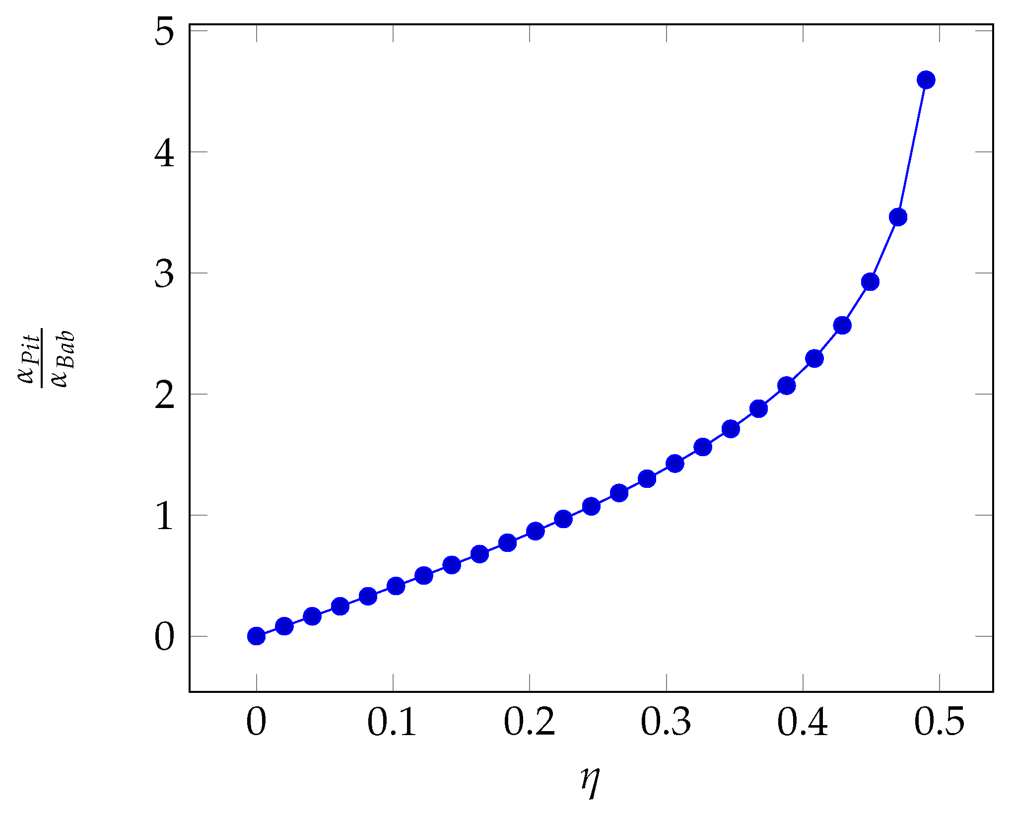
In
Figure 1, we can see that the perturbation factor is lower than 1 for
but can be significantly larger than 1 for higher probability premium values. We have therefore
.
The resulting premiums
and
using
and
for the specific risk-aversion coefficient are respectively
3. Comparison of Premiums
In
Section 2, we have derived the premium under two different approximation levels. We wish to see if the more accurate fourth-order approximation entails a higher premium, i.e., if the use of the usual second-order approximation results in an underestimated premium, which may be dangerous for the insurer. Though overestimation is similarly dangerous, here we take the viewpoint of the insurer, for which premium overestimation is the lesser problem, since it may result in a reduced number of insurance subscriptions. In the following, we limit ourselves to consider underestimation. In this section, we compare the two expressions and look for the conditions where that happens. Throughout this section, the number
n of claims will be considered to be a fixed quantity; this limitation will be removed in
Section 4.
From the two expressions (
11) and (
12), we can form their ratio
We consider the case when setting the premium through the usual second-order approximation can lead to underestimating the premium; we focus on underestimation, since it is the more dangerous error of the two (under- vs overestimation), leading to the possibility that premiums do not cover losses. Going back to Equation (
17), we see that we have underestimation when
. Therefore, whether the fourth-order premium is larger or not than its second-order counterpart depends just on the sign and relative values of the skewness and kurtosis of the loss. In
Table 2, we report the general conditions for underestimation of the premium when we stop at the second-order approximation. In two out of four cases (same signs for skewness and kurtosis), the conclusions are general. In the other two cases, the possibility of underestimation depends on the specific distribution of losses. Since we must have
for underestimation, the underestimation condition can be formulated as
Since the overall loss is determined by the accrual of losses over the single events, we can derive a condition on the statistics of any single event by recalling that
where
is the loss suffered during th
i-th event and
n is the overall number of events (and therefore claims), with
,…,
being i.i.d. random variables.
Due to the i.i.d. nature of the
variables, the skewness and the kurtosis of the random variable
X may be derived from that of the loss in any single event (see [
28]):
The underestimation condition can then be reformulated as follows, by replacing Equation (
20) in Equation (
18):
3.1. Premium Underestimation for Major Distributions
It is interesting to analyze if the underestimation condition, as ascertained through
Table 2 or Equation (
18), is met for the commonest distribution of losses. In particular, we consider the following distributions: Generalized Pareto (GPD), Lognormal, Gamma, Pareto. The main features of those distributions are shown in
Table 3, while their skewness and kurtosis are reported in
Table 4 [
29,
30,
31].
We now examine the underestimation condition for each distribution.
For the Generalized Pareto distribution, we see from
Table 4 that both the skewness and the kurtosis are positive under the same conditions for the existence of finite skewness and kurtosis (the shape parameter must be lower than 1/3 and 1/4 respectively), so that we fall into the underestimation condition of
Table 2.
Similarly, for the lognormal distribution, we have positive skewness and kurtosis. In particular, the kurtosis is always larger than 3. The second-order premium is an underestimate again.
For the Gamma distribution, the positivity of the shape parameter a implies that both the skewness and the kurtosis are positive, ending up again under the underestimation case.
Finally, for the Pareto distribution, the conditions for the existence of finite skewness and kurtosis guarantee the positive of both central moments and therefore the underestimation.
We can then conclude that for all these 4 common distributions, stopping at the second order in the premium computation leads us to underestimate the actual premium.
3.2. Premium Uncertainty
So far, we have assumed that the insurer can compute the premium if it knows the distribution of losses. However, such knowledge is typically approximate, since the insurer will typically estimate the parameters of the loss model based on observations. Consequently, the premium computed according to Equations (
11) or (
12) will be just an approximation of the correct value. It is important to quantify the uncertainty associated with the premium since that is an additional source of error, which may even mask the error due to a lower-order approximation. In this section, we compute the uncertainty in the premium due to an approximate knowledge of the loss distribution parameters.
Since the computation of the premium is carried out through a complex function, we resort to a Taylor series approximation of that function by considering it as a function of the loss distribution parameters. The expansion is performed around the expected values of those parameters. All the distributions considered so far rely on two parameters so that we can write the Taylor series expansion
of the premium by adopting the following generic notation
where
x and
y are the estimates of the two parameters, and
and
are their expected values. If we stop at the first order, we get
In the following, the parameters of the distributions of interest will be considered to be random variables to describe their uncertainty, so that the premium (from now on we use the generic symbol P) is a random variable as well. To gauge the uncertainty on the premium, we will compute its variance. As a simplifying assumption, we consider the estimates of the two parameters as independent of each other, though they will be typically estimated on the same sample of observations.
The general expression for the variance of
P is then
We can now compute the variance of the premium for the loss distributions we have reported in
Table 3.
After recalling the premium expressions for the Pareto distribution
we can get the variances, by indicating with
e
the expected values of the two parameters
Similarly, for the Generalized Pareto distribution we get
and consequently, we get the variances
Under the gamma distribution, we have instead:
so that the variances are
Finally, for the lognormal distribution we have
and the variances are
3.3. An Application to Realistic Cases
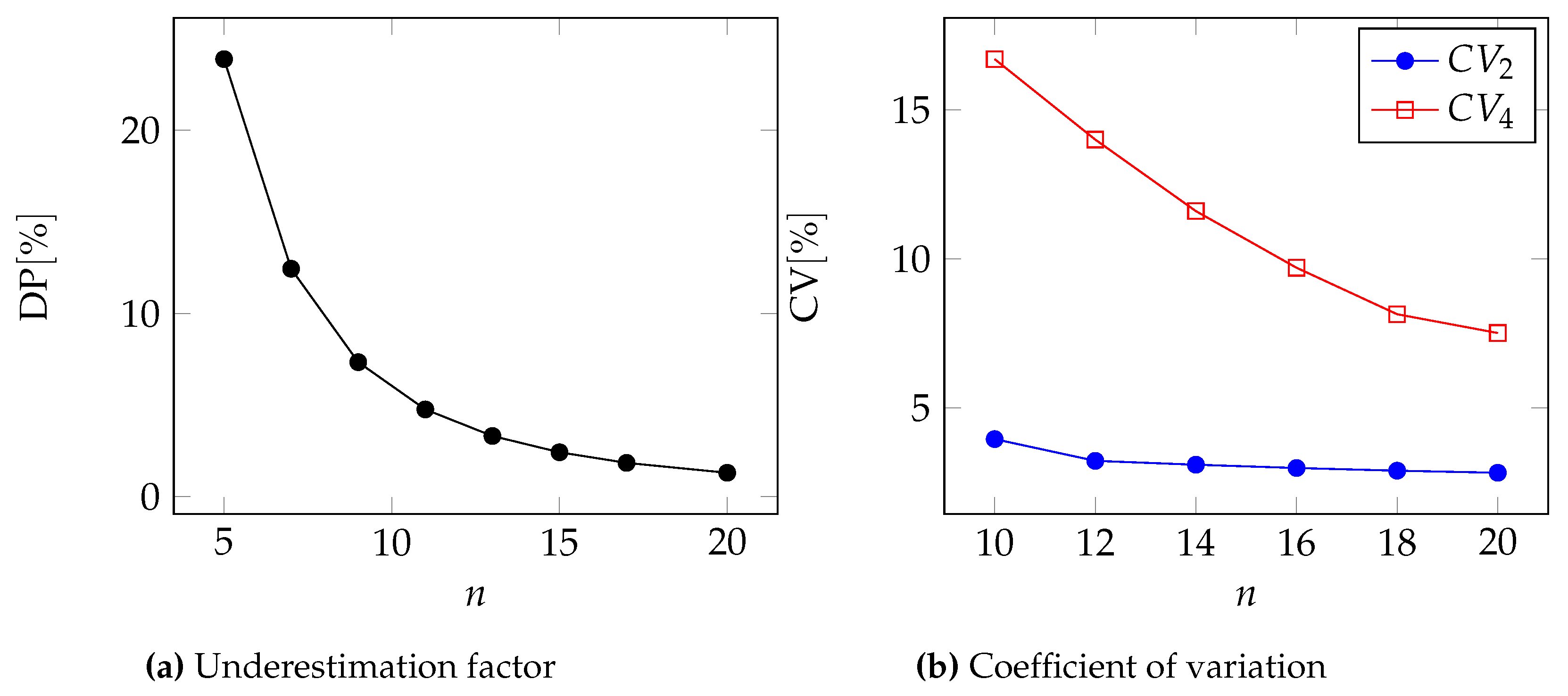
In the previous sections, we have derived two metrics (underestimation factor and premium estimator variance) that allow us to compare the insurance premium as computed at two different approximation levels: second and fourth order. In this section, we get a feeling of how the two approximation levels compare in realistic cases, i.e., when the loss distribution parameters take realistic values.
For this purpose, we consider the parameter values obtained in [
6,
30,
31], which we report in
Table 5. In particular, the Generalized Pareto distribution describes the duration (in minutes) of a cloud service outage, where the amount of economic losses is proportional to the duration of the outage. The lognormal distribution describes the severity of the losses due to a cyber-attack by a hacker. The Gamma distribution describes the severity of the losses due to a natural catastrophe (as a hurricane). The Pareto distribution is one of the most used distributions in the literature to describe the severity of losses in many cases, for example, losses due to fire damages, car accidents, and ICT service failures.
All the cases we consider here refer to a policy duration of one year, and assume full compensation. In this section, we adopt the Babcock method with
to determine the risk-aversion coefficient. As assumed in
Section 3.2, for the sake of computing the premium uncertainty, the loss distribution parameters are considered to be random variables. We plug their estimators, assumed to be unbiased and with a standard deviation equal to 1% of their expected value (this value is taken as a reference for convenience, but it should be assessed for the specific case at hand), in the premium computation formula.
To compare the two approximations, we first compute the underestimation factor through the percentage relative difference of the premiums, assuming that the distribution parameters are known exactly:
As a second metric for comparison, we compute the coefficient of variation (i.e., the ratio of standard deviation to expected value) for the two approximation levels. We obviously wish that coefficient to be as low as possible.
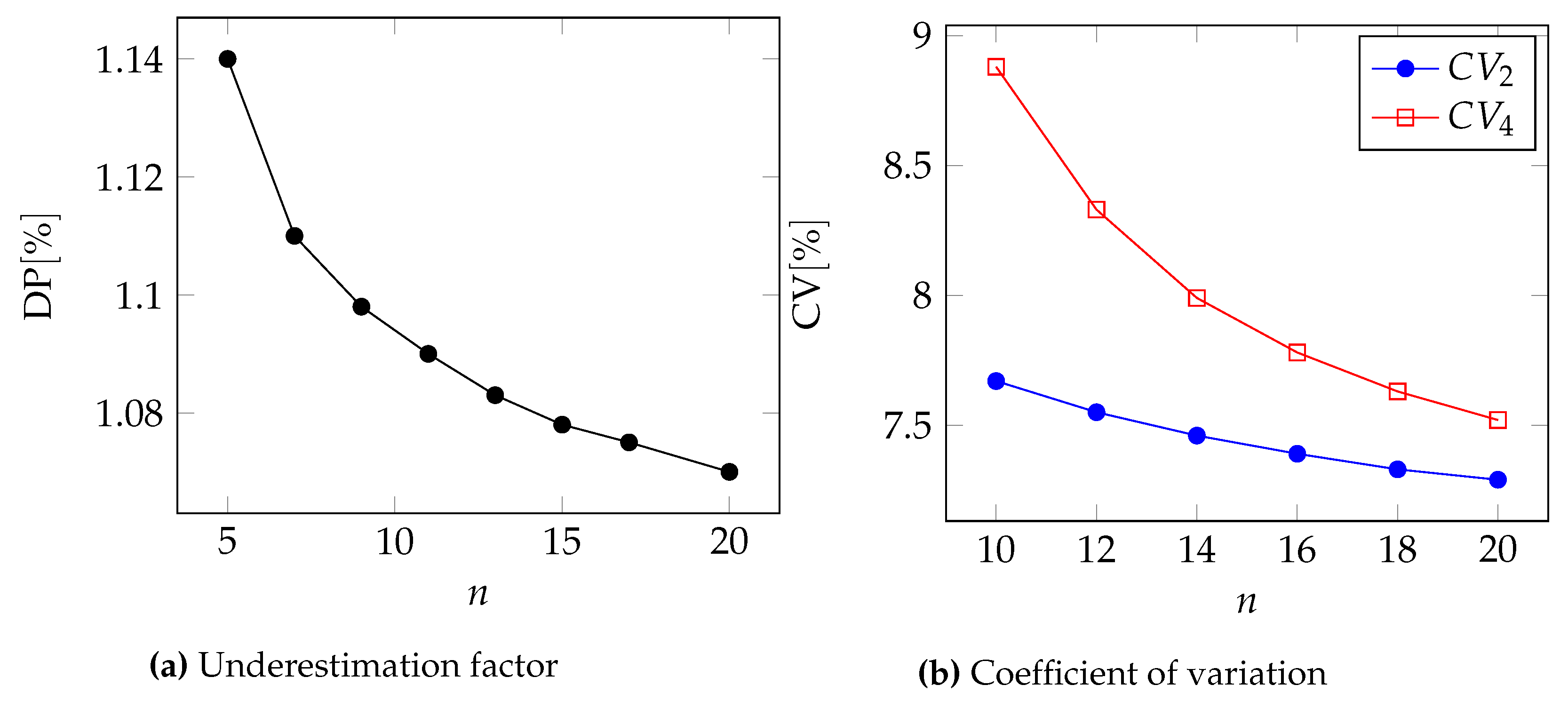
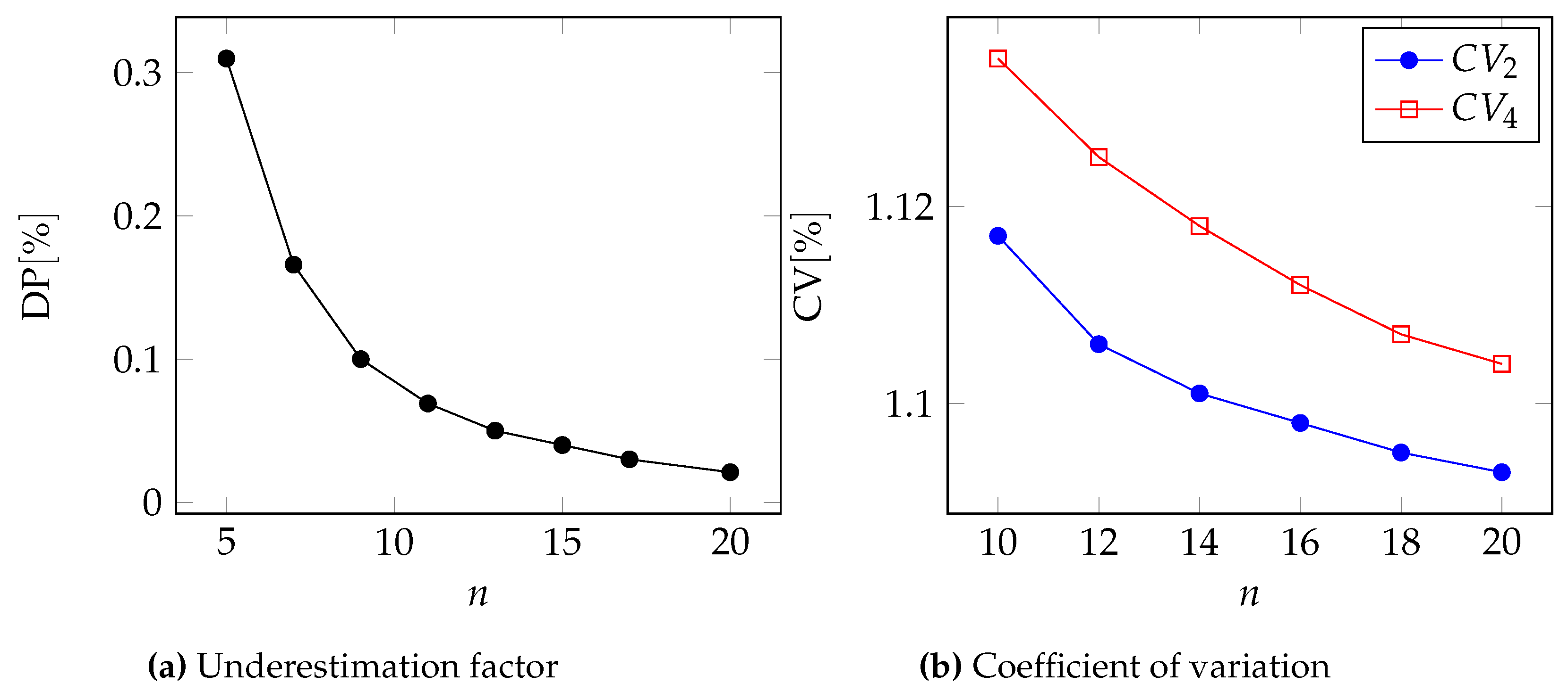
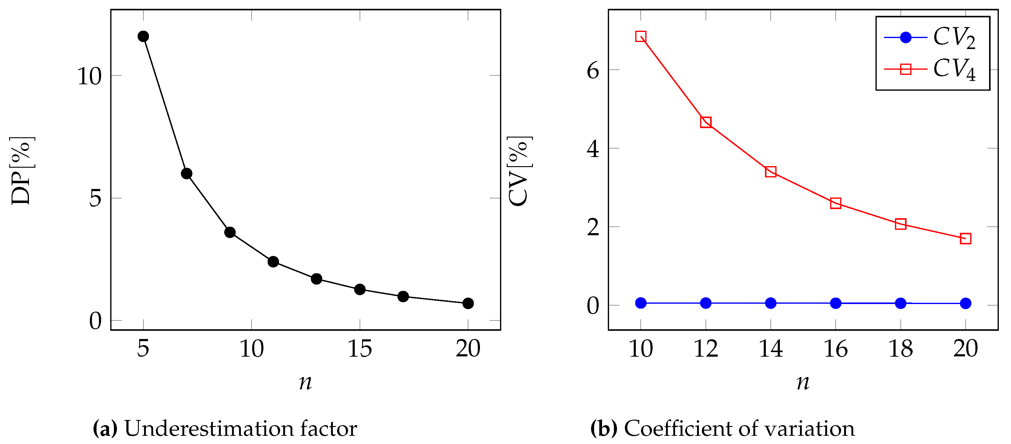
In
Figure 2,
Figure 3,
Figure 4 and
Figure 5, we can see the two metrics to compare the two approximations for the Pareto, GPD, Gamma, and Lognormal distributions respectively.
Moreover, in
Table 6 and
Table 7, we report the underestimation DP and the coefficient of variation for two different values of the number of events
n.
In all cases, we can see that .
Naturally, using
(therefore also
) the difference
between the two approximation levels tends to zero
In fact, for large values of
n,
. Instead, if
is a fixed real constant, the relative difference
is always positive and does not depend on the number of events
n:
4. Insurer’s Risk
As in any total coverage insurance scheme, the insured is held indemnified against any damage by just paying the premium. On the other hand, the insurer must cover all the losses the insured suffers. Since the premium is a fixed quantity and the loss is a random variable, the insurer incurs the risk of paying more than what is cashed in. Of course, this risk is different for the two approximation levels we have considered so far. It is larger for the second-order approximation as long as its premium is lower than the fourth-order approximation. In this section, we quantify that risk by computing the Value-at-Risk (VaR), also considering the number n of events as a random variable.
The Value-at-Risk is a well-known measure of risk, defined first in the financial world and then extended to other fields. For example, it has been employed in the ICT sector in [
3,
32,
33]. In our case, the Value-at-Risk at the confidence level
is the smallest number
such that the probability that the loss
X exceeds
is not larger than
[
34]:
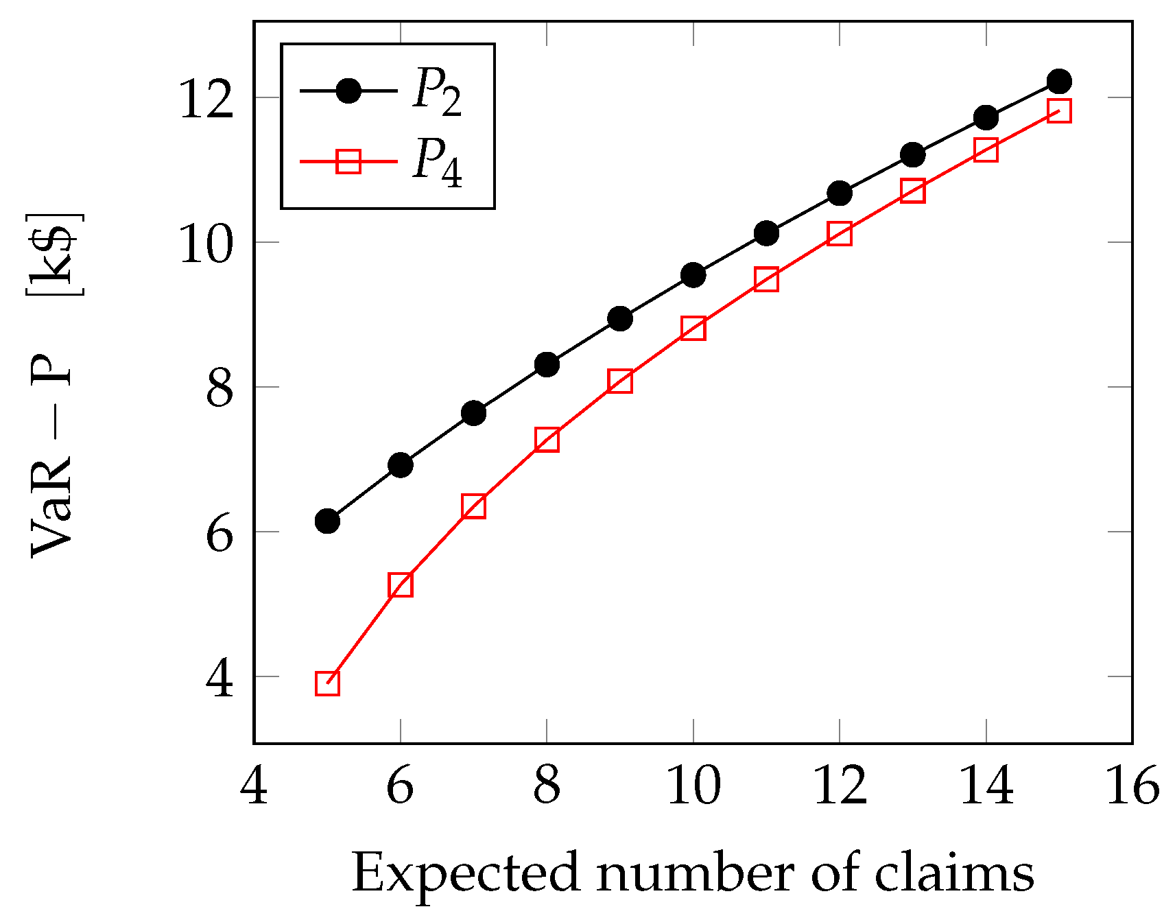
We can now compute the VaR for the four distributions we have considered so far. For the sake of simplicity, we use the notation , to represent the insurance premium. In the following, the number of claims n is considered to follow a Poisson random variable with parameter , where refers to the frequency of the claims, and T is the length of the observation period. The losses taking place over the sequence of events are assumed to be i.i.d. random variables.
Lognormal case: For the case of the lognormal distribution we use Wilkinson’s method as employed in [
35] to estimate the queue of lognormal sums. They assume that the sum of lognormal variables is still lognormal. So that the overall loss
follows a lognormal distribution, in particular
, with
Z being a Gaussian variable with mean
and variance
, which we can compute using Wald identity:
The Value-at-Risk can therefore be determined as follows
where
is the cumulative distribution function of a standard (zero-mean, unit-variance) Gaussian random variable. In
Figure 6, we see how the extreme loss (i.e., the difference between the Value-at-Risk and the premium) grows with the expected number of claims
.
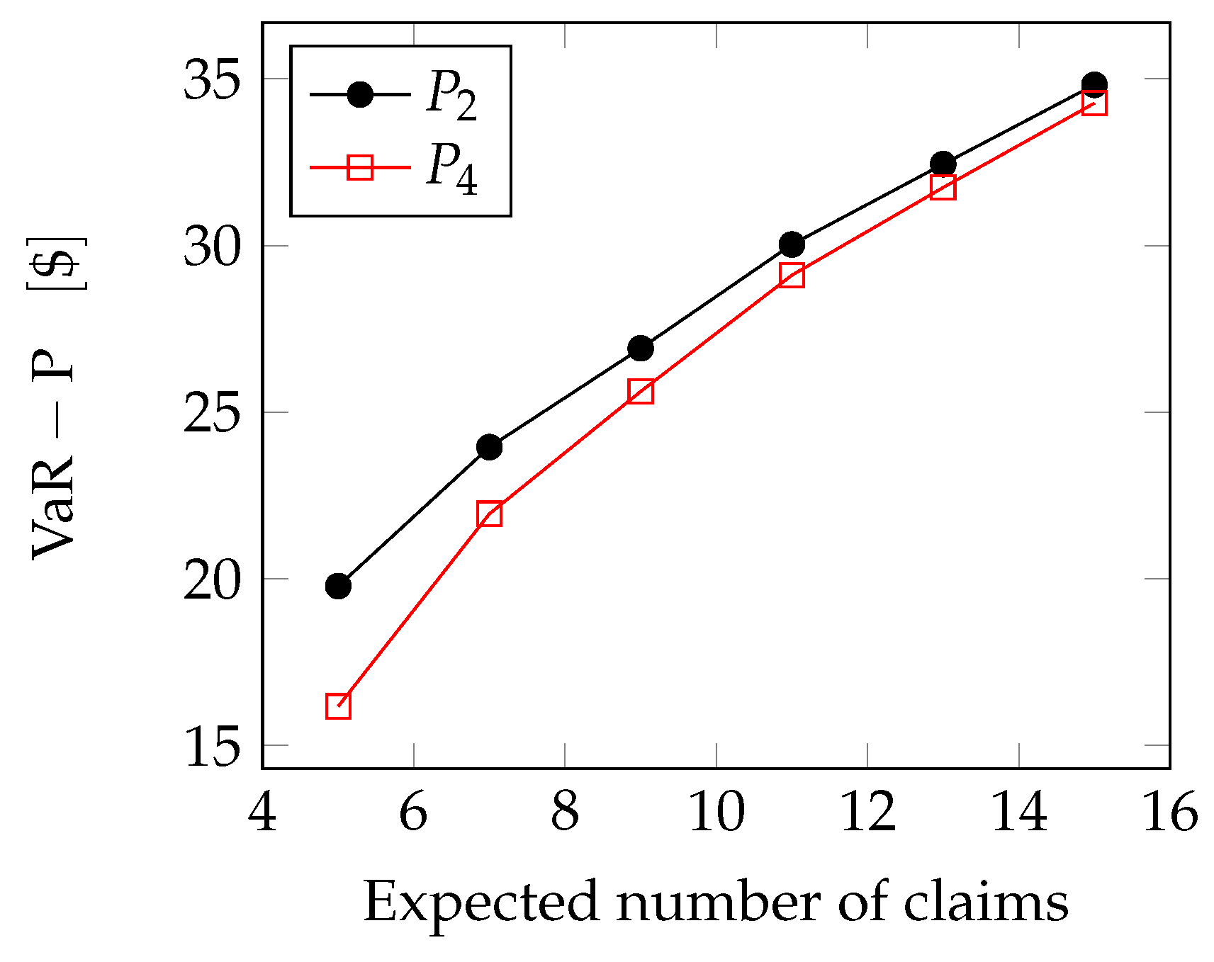
Pareto case: In the Pareto and GPD cases, we can use the Generalized Extreme Value Theory [
36,
37,
38] to compute the VaR.
As can be seen, for example, in [
39], we can approximate the sum of
n i.i.d. Pareto-distributed variables through a Generalized Extreme Value (GEV) variable, so that the overall loss
X exhibits the probability density function
where
and
,
and
are the location, scale and shape parameter of the GEV distribution.
is a parameter that governs the shape of the tail under consideration: the fatness of the tail will then depend on the exact value assumed by it. We can observe that
is related to the number of events
n, in fact, when
n increases, it changes the slope of the distribution and consequently also
. The most used range in which
is found is
. In our case, we estimate the location scale and shape parameters through an R-package (ismev). Therefore, if
p is the probability that an event occurs, the quantile function for GEV distribution is
Assuming
, we can compute the VaR as follows.
In
Figure 7, we see how the extreme loss grows with the number of claims: the extreme loss is anyway lower for the fourth-order approximation.
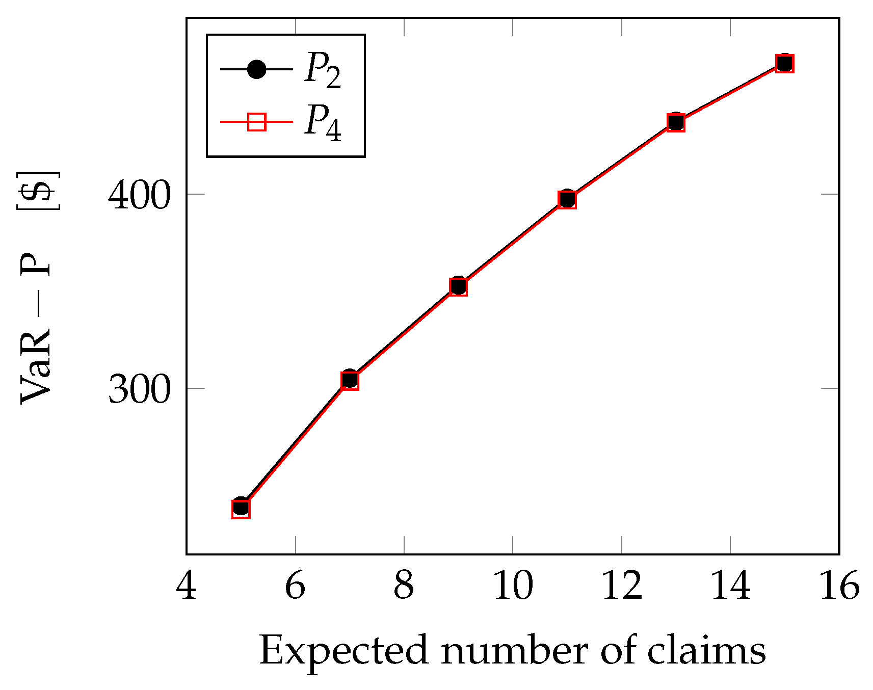
GPD case:
Now, using the same arguments that we adopted for Pareto case, we can find the VaR for the GPD case.
In
Figure 8 the curves are actually very close but not coincident, because the difference in percentage between the two premiums,
and
, is very low.
Gamma case: Since
, again using Wald’s identity and the property of the Gamma distribution, the overall loss
X is also
distribution with mean
and variance
. If we assume that
, the loss
X can be approximated by a normal distribution with the same mean and variance, so that
. We can then estimate the Value-at-Risk as follows
As can be seen in
Figure 9, the extreme loss grows with the number of claims, but is lower for the fourth-order approximation.
5. Conclusions
In this work, we have focused our attention on the comparison of insurance premium when they are computed under the expected utility principle based on two approximation levels for the loss statistics: second-order (mean-variance) vs fourth-order (mean-variance-skewness-kurtosis).
We have shown that for the major cases of interest, computing the premium based on the second-order approximation is riskier for the insurer, since the premium is lower.
However, if we take into account the possibility of incorrectly estimating the higher-order statistics involved in the fourth-order approximation, the comparison outcome may be reversed. In fact, the dispersion in the fourth-order premium may be so high as to have too high a premium. A higher premium would probably divert prospective customers away from subscribing an insurance policy.
A tentative conclusion is then to use the fourth-order approximation to compute the insurance premium as long as the estimate of the fourth-order statistics is sufficiently accurate.


