How to Identify Varying Lead–Lag Effects in Time Series Data: Implementation, Validation, and Application of the Generalized Causality Algorithm


Abstract
1. Introduction
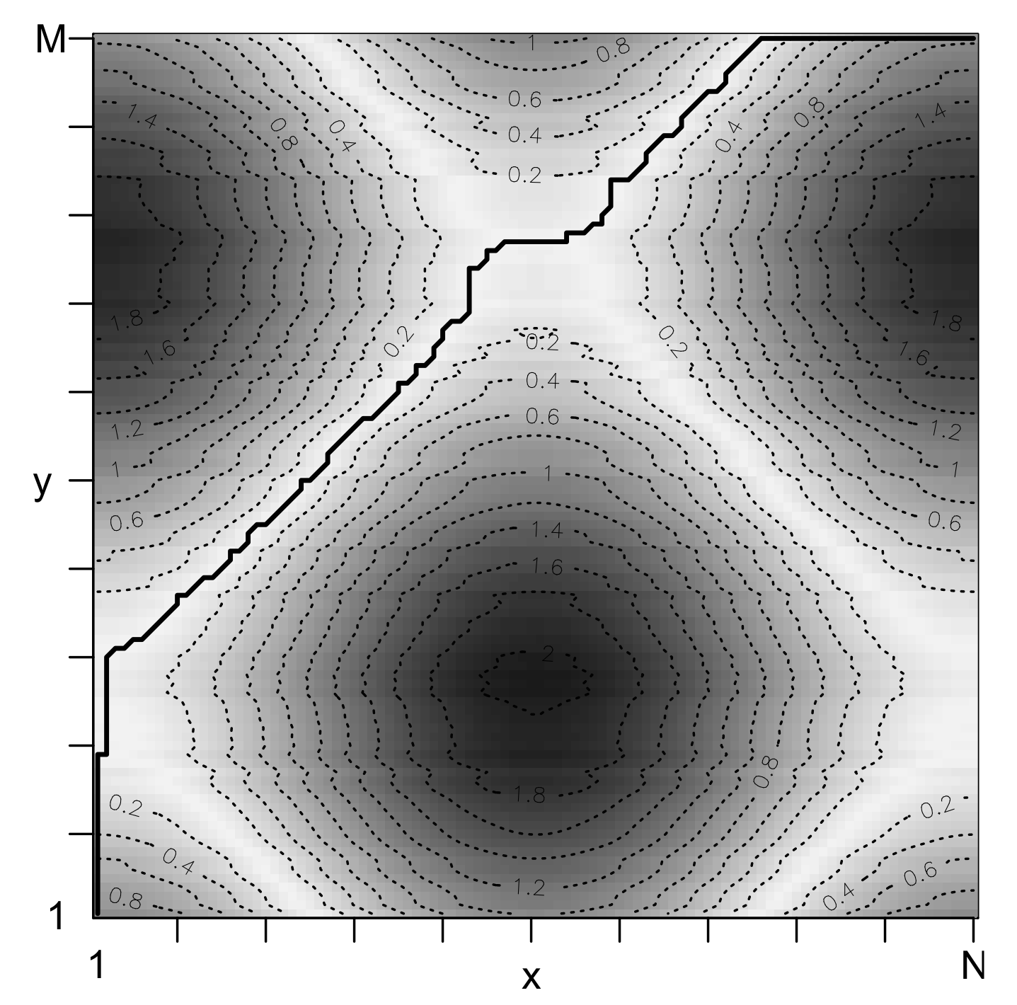
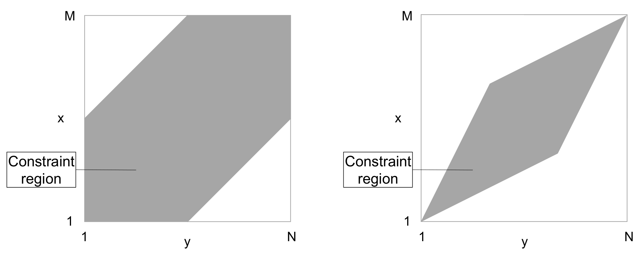
2. Theoretical Concept
- and (Boundary condition).
- and (Monotonicity condition).
- (Step size condition).
3. Generalized Causality Algorithm
3.1. Methodology
| Algorithm 1 Generalized causality algorithm |
|
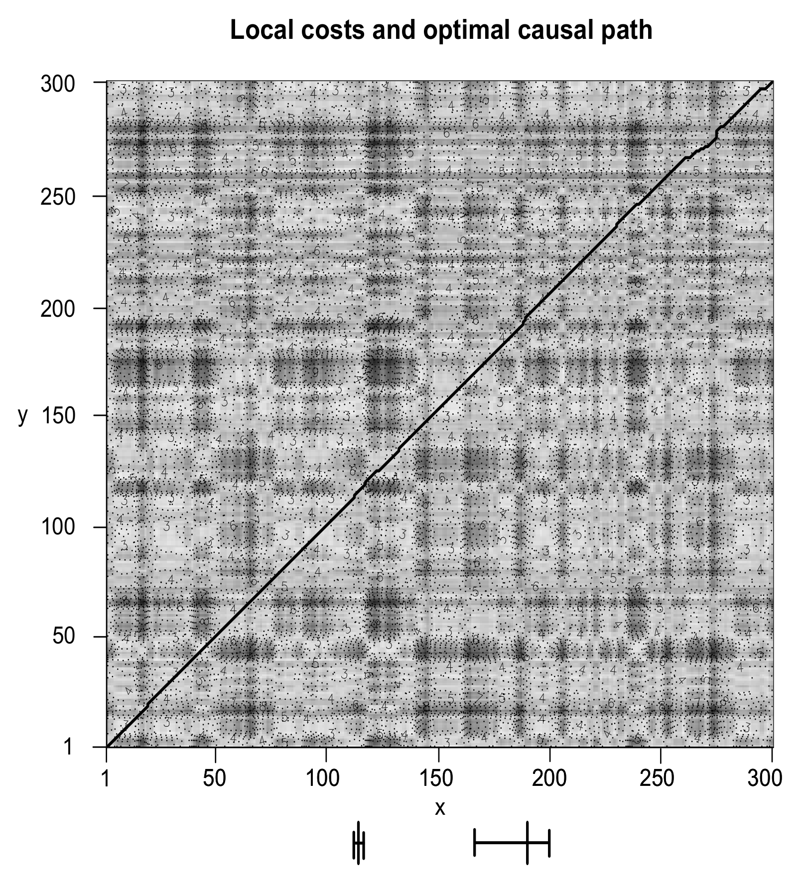
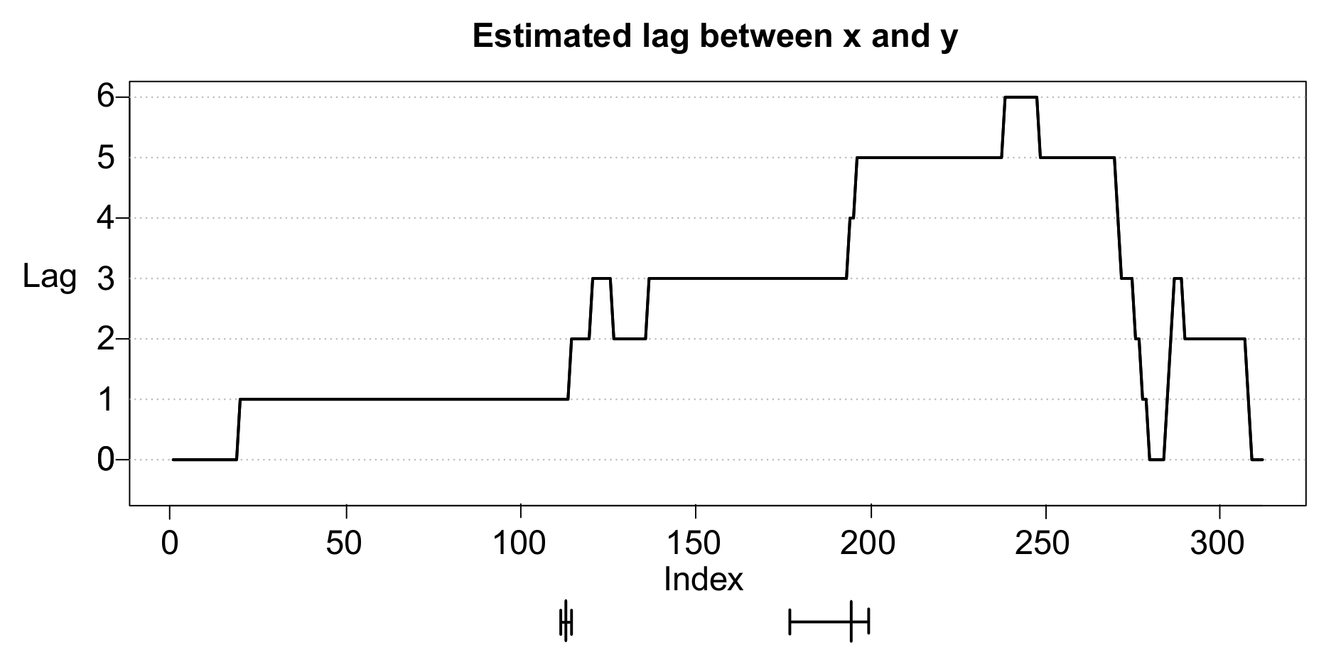
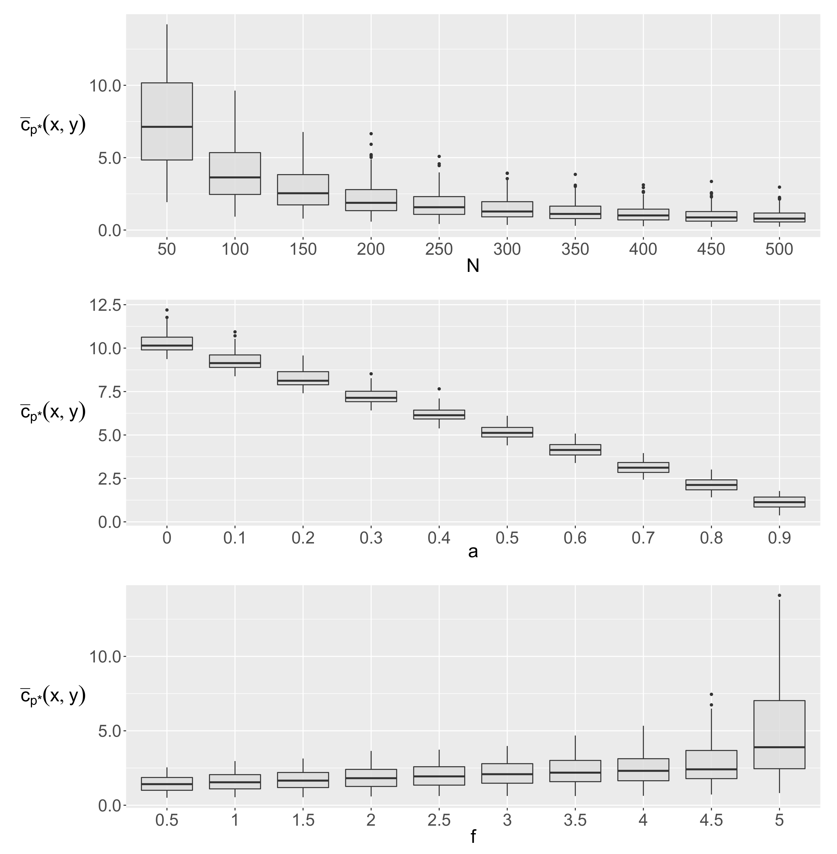
3.2. Simulation Study
- The first phase () contains 100 data points () where X leads Y by 1 lag () with a “strength” of .
- The second phase () contains 100 data points () where X leads Y by 3 lags () with a “strength” of .
- The third phase () contains 100 data points () where X leads Y by 5 lags () with a “strength” of .
4. Applications to Real Data
4.1. Data set
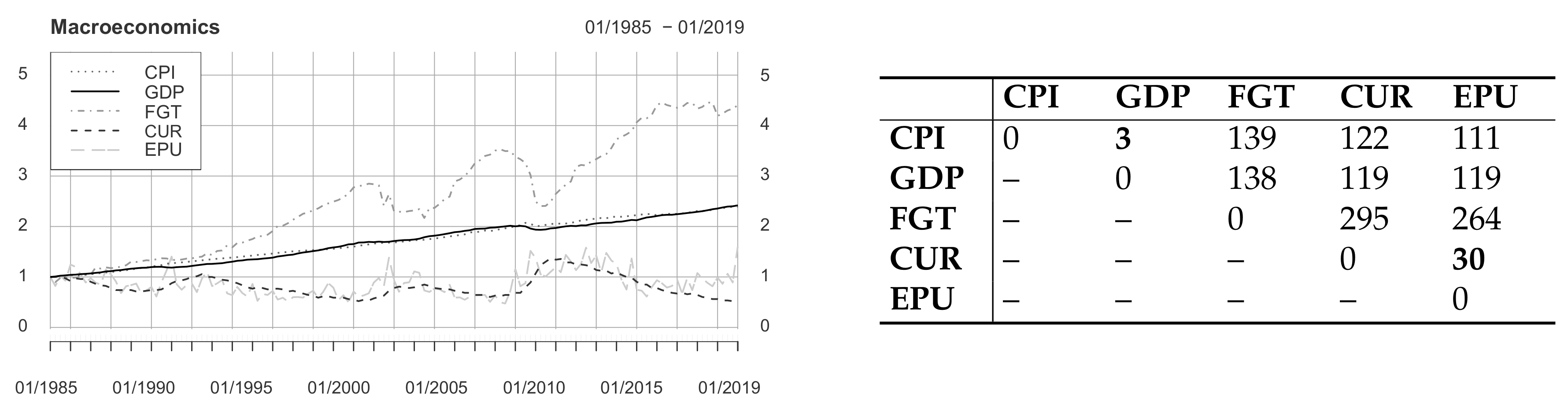
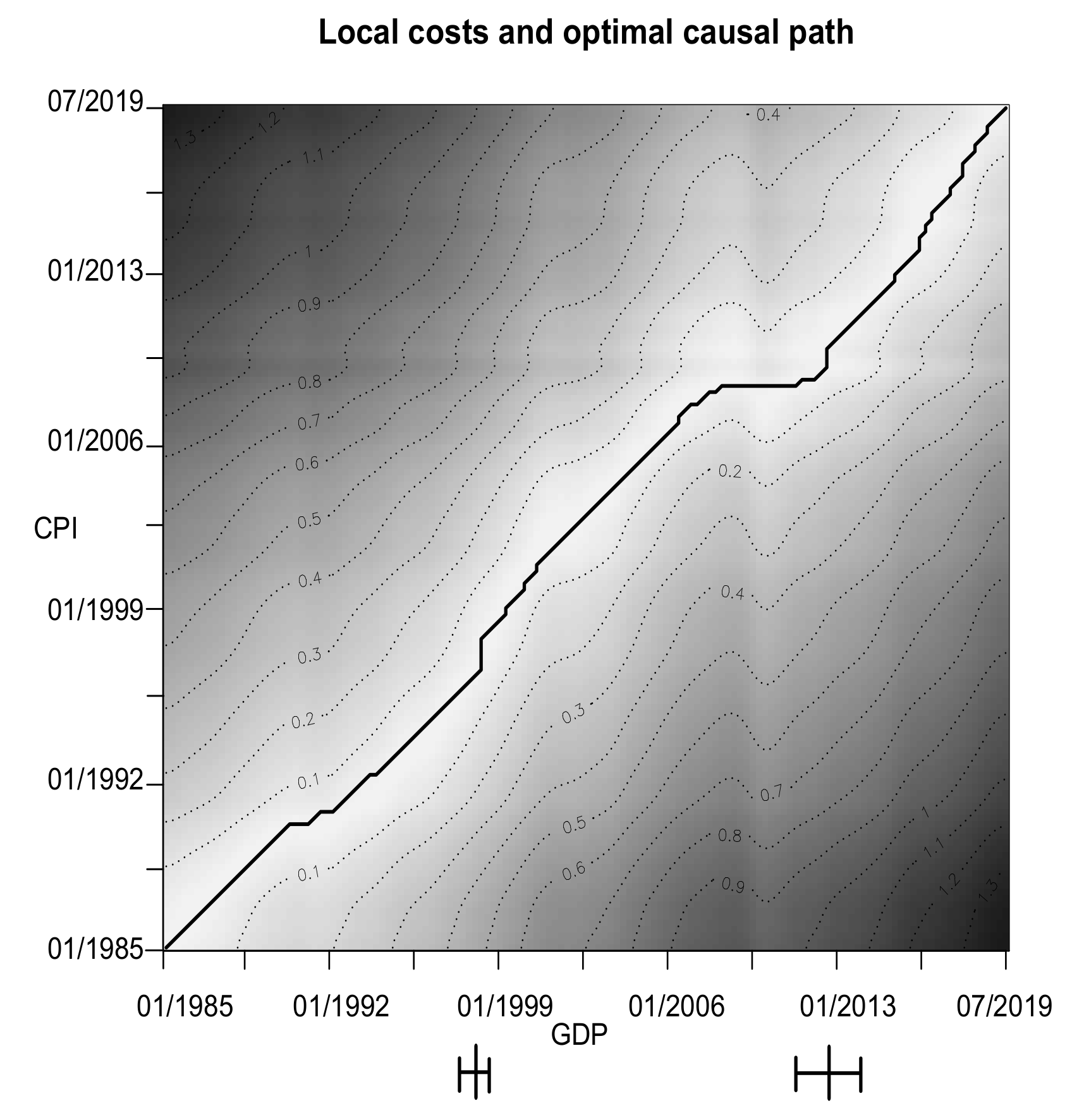
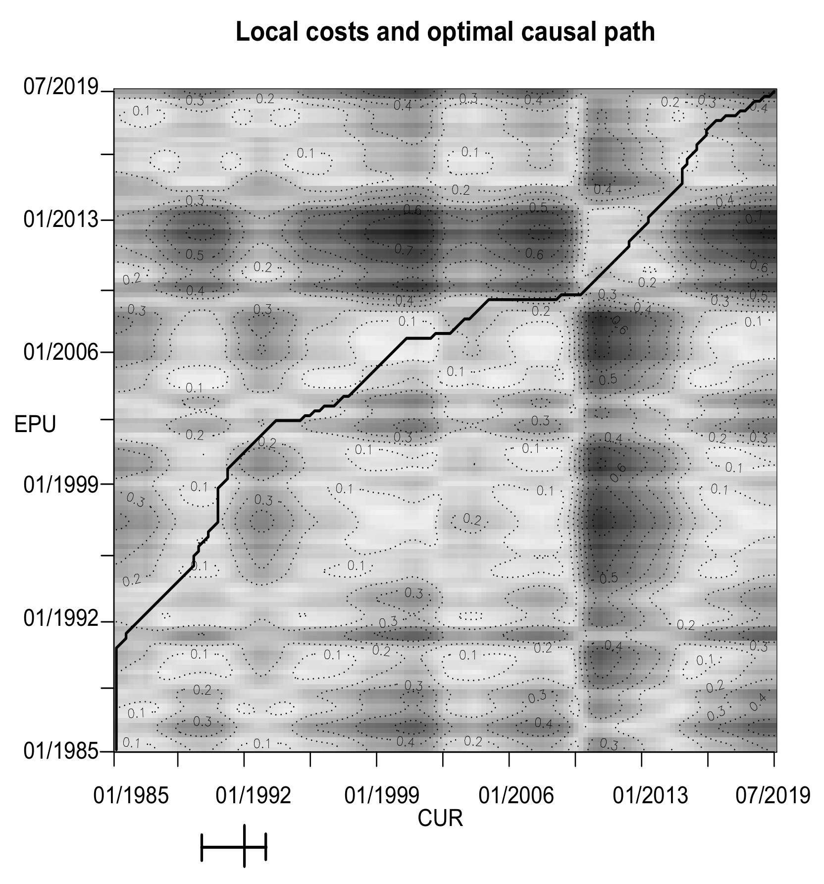
4.2. Macroeconomics
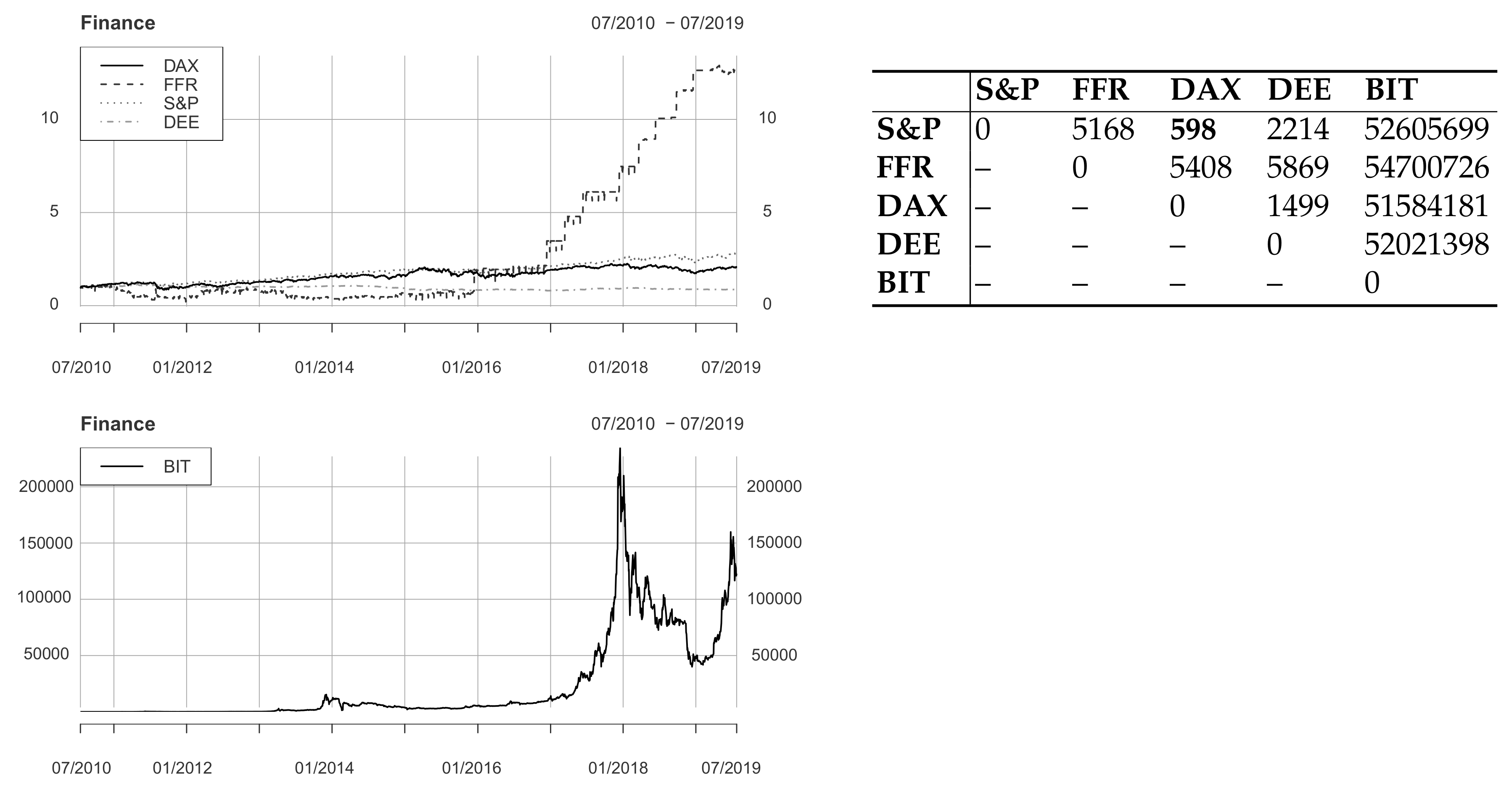
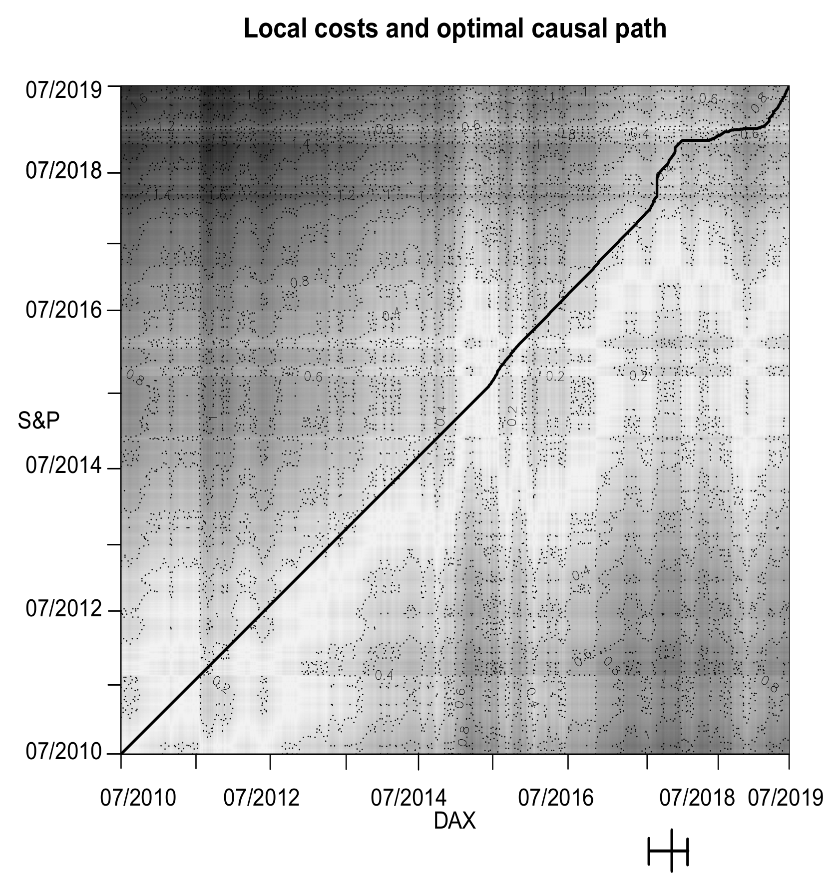
4.3. Finance
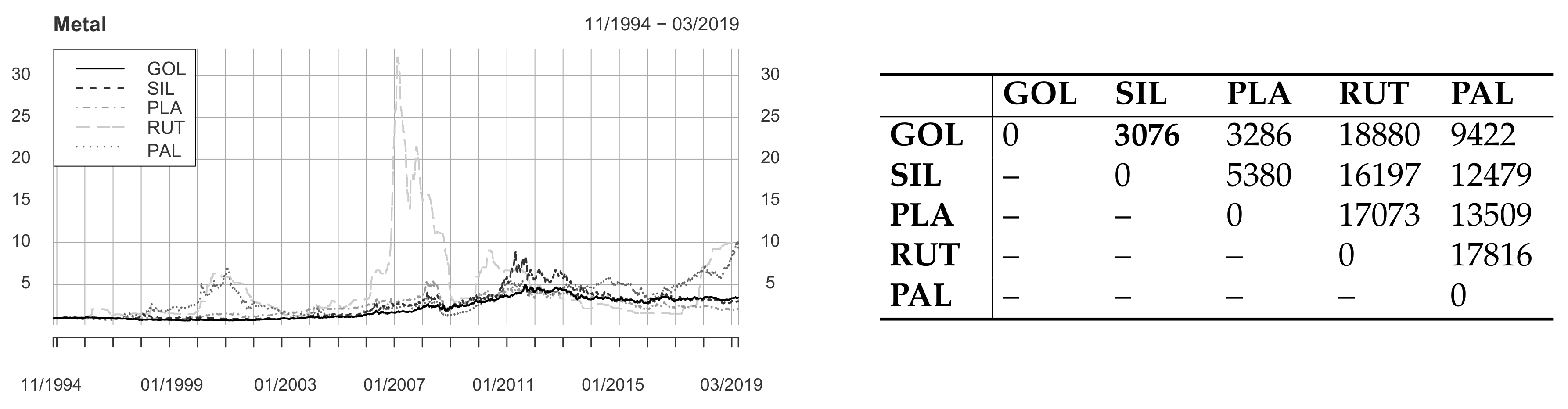
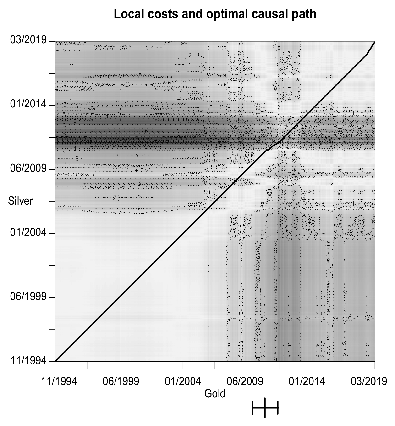
4.4. Metal
5. Conclusions
Author Contributions
Funding
Acknowledgments
Conflicts of Interest
References
- Gauthier, T.D. Detecting trends using Spearman’s rank correlation coefficient. Environ. Forensics 2001, 2, 359–362. [Google Scholar] [CrossRef]
- Mudelsee, M. Estimating Pearson’s correlation coefficient with bootstrap confidence interval from serially dependent time series. Math. Geol. 2003, 35, 651–665. [Google Scholar] [CrossRef]
- Gatev, E.; Goetzmann, W.N.; Rouwenhorst, K.G. Pairs trading: Performance of a relative-value arbitrage rule. Rev. Financ. Stud. 2006, 19, 797–827. [Google Scholar] [CrossRef]
- Batista, G.E.; Wang, X.; Keogh, E.J. A complexity-invariant distance measure for time series. In Proceedings of the 2011 SIAM International Conference on Data Mining; Liu, B., Liu, H., Clifton, C.W., Washio, T., Kamath, C., Eds.; Society for Industrial and Applied Mathematics: Philadelphia, PA, USA, 2011; pp. 699–710. [Google Scholar]
- Stübinger, J.; Endres, S. Pairs trading with a mean-reverting jump-diffusion model on high-frequency data. Quant. Financ. 2018, 18, 1735–1751. [Google Scholar] [CrossRef]
- Knoll, J.; Stübinger, J.; Grottke, M. Exploiting social media with higher-order factorization machines: Statistical arbitrage on high-frequency data of the S&P 500. Quant. Financ. 2019, 19, 571–585. [Google Scholar]
- Ding, H.; Trajcevski, G.; Scheuermann, P.; Wang, X.; Keogh, E.J. Querying and mining of time series data: Experimental comparison of representations and distance measures. In Proceedings of the VLDB Endowment; Jagadish, H.V., Ed.; ACM: New York, NY, USA, 2008; pp. 1542–1552. [Google Scholar]
- Wang, G.J.; Xie, C.; Han, F.; Sun, B. Similarity measure and topology evolution of foreign exchange markets using dynamic time warping method: Evidence from minimal spanning tree. Phys. A Stat. Mech. Its Appl. 2012, 391, 4136–4146. [Google Scholar] [CrossRef]
- Stübinger, J. Statistical arbitrage with optimal causal paths on high-frequency data of the S&P 500. Quant. Financ. 2019, 19, 921–935. [Google Scholar]
- Juang, B.H. On the hidden Markov model and dynamic time warping for speech recognition—A unified view. Bell Labs Tech. J. 1984, 63, 1213–1243. [Google Scholar] [CrossRef]
- Rath, T.M.; Manmatha, R. Word image matching using dynamic time warping. In Proceedings of the IEEE Computer Society Conference on Computer Vision and Pattern Recognition; Dyer, C., Perona, P., Eds.; IEEE: Danvers, MA, USA, 2003; pp. 521–527. [Google Scholar]
- Muda, L.; Begam, M.; Elamvazuthi, I. Voice recognition algorithms using mel frequency cepstral coefficient (MFCC) and dynamic time warping (DTW) techniques. J. Comput. 2010, 2, 138–143. [Google Scholar]
- Arici, T.; Celebi, S.; Aydin, A.S.; Temiz, T.T. Robust gesture recognition using feature pre-processing and weighted dynamic time warping. Multimed. Tools Appl. 2014, 72, 3045–3062. [Google Scholar] [CrossRef]
- Cheng, H.; Dai, Z.; Liu, Z.; Zhao, Y. An image-to-class dynamic time warping approach for both 3D static and trajectory hand gesture recognition. Pattern Recognit. 2016, 55, 137–147. [Google Scholar] [CrossRef]
- Jiao, L.; Wang, X.; Bing, S.; Wang, L.; Li, H. The application of dynamic time warping to the quality evaluation of Radix Puerariae thomsonii: Correcting retention time shift in the chromatographic fingerprints. J. Chromatogr. Sci. 2014, 53, 968–973. [Google Scholar] [CrossRef] [PubMed]
- Dupas, R.; Tavenard, R.; Fovet, O.; Gilliet, N.; Grimaldi, C.; Gascuel-Odoux, C. Identifying seasonal patterns of phosphorus storm dynamics with dynamic time warping. Water Resour. Res. 2015, 51, 8868–8882. [Google Scholar] [CrossRef]
- Rakthanmanon, T.; Campana, B.; Mueen, A.; Batista, G.; Westover, B.; Zhu, Q.; Zakaria, J.; Keogh, E.J. Searching and mining trillions of time series subsequences under dynamic time warping. In Proceedings of the 18th ACM SIGKDD International Conference on Knowledge Discovery and Data Mining; Yang, Q., Ed.; ACM: New York, NY, USA, 2012; pp. 262–270. [Google Scholar]
- Fu, C.; Zhang, P.; Jiang, J.; Yang, K.; Lv, Z. A Bayesian approach for sleep and wake classification based on dynamic time warping method. Multimed. Tools Appl. 2017, 76, 17765–17784. [Google Scholar] [CrossRef]
- Stübinger, J.; Schneider, L. Epidemiology of coronavirus COVID-19: Forecasting the future incidence in different countries. Healthcare 2020, 8, 99. [Google Scholar] [CrossRef]
- Chinthalapati, V.L. High Frequency Statistical Arbitrage via the Optimal Thermal Causal Path; Working Paper; University of Greenwich: London, UK, 2012. [Google Scholar]
- Kim, S.; Heo, J. Time series regression-based pairs trading in the Korean equities market. J. Exp. Theor. Artif. Intell. 2017, 29, 755–768. [Google Scholar] [CrossRef]
- Ghysels, E. A Time Series Model with Periodic Stochastic Regime Switching; Université de Montréal: Montreal, QC, Canada, 1993. [Google Scholar]
- Bock, M.; Mestel, R. A regime-switching relative value arbitrage rule. In Operations Research Proceedings 2008; Fleischmann, B., Borgwardt, K.H., Klein, R., Tuma, A., Eds.; Springer: Berlin/Heidelberg, Germany, 2009; pp. 9–14. [Google Scholar]
- Xi, X.; Mamon, R. Capturing the regime-switching and memory properties of interest rates. Comput. Econ. 2014, 44, 307–337. [Google Scholar] [CrossRef]
- Endres, S.; Stübinger, J. Regime-switching modeling of high-frequency stock returns with Lévy jumps. Quant. Financ. 2019, 19, 1727–1740. [Google Scholar] [CrossRef]
- Shi, Y.; Feng, L.; Fu, T. Markov regime-switching in-mean model with tempered stable distribution. Comput. Econ. 2019, 12, 105. [Google Scholar] [CrossRef]
- Ghysels, E. Macroeconomics and the reality of mixed frequency data. J. Econ. 2016, 193, 294–314. [Google Scholar] [CrossRef]
- Kuzin, V.; Marcellino, M.; Schumacher, C. MIDAS vs. mixed-frequency VAR: Nowcasting GDP in the euro area. Int. J. Forecast. 2011, 27, 529–542. [Google Scholar] [CrossRef]
- Geweke, J.; Amisano, G. Optimal prediction pools. J. Econ. 2011, 164, 130–141. [Google Scholar] [CrossRef]
- Del Negro, M.; Hasegawa, R.B.; Schorfheide, F. Dynamic prediction pools: An investigation of financial frictions and forecasting performance. J. Econ. 2016, 192, 391–405. [Google Scholar] [CrossRef]
- McAlinn, K.; West, M. Dynamic Bayesian predictive synthesis in time series forecasting. J. Econ. 2019, 210, 155–169. [Google Scholar] [CrossRef]
- McAlinn, K.; Aastveit, K.A.; Nakajima, J.; West, M. Multivariate Bayesian predictive synthesis in macroeconomic forecasting. J. Am. Stat. Assoc. 2019. [Google Scholar] [CrossRef]
- Sornette, D.; Zhou, W.X. Non-parametric determination of real-time lag structure between two time series: The “optimal thermal causal path” method. Quant. Financ. 2005, 5, 577–591. [Google Scholar] [CrossRef]
- Zhou, W.X.; Sornette, D. Non-parametric determination of real-time lag structure between two time series: The “optimal thermal causal path” method with applications to economic data. J. Macroecon. 2006, 28, 195–224. [Google Scholar] [CrossRef]
- Müller, M. Information Retrieval for Music and Motion; Springer: Berlin/Heidelberg, Germany, 2007. [Google Scholar]
- Keogh, E.J.; Ratanamahatana, C.A. Exact indexing of dynamic time warping. Knowl. Inf. Syst. 2005, 7, 358–386. [Google Scholar] [CrossRef]
- Li, Q.; Clifford, G.D. Dynamic time warping and machine learning for signal quality assessment of pulsatile signals. Physiol. Meas. 2012, 33, 1491–1502. [Google Scholar] [CrossRef]
- Vlachos, M.; Kollios, G.; Gunopulos, D. Discovering similar multidimensional trajectories. In Proceedings of the 18th International Conference on Data Engineering; Agrawal, R., Dittrich, K., Eds.; IEEE: Washington, DC, USA, 2002; pp. 673–684. [Google Scholar]
- Senin, P. Dynamic Time Warping Algorithm Review; Working Paper; University of Hawaii at Manoa: Honolulu, HI, USA, 2008. [Google Scholar]
- Coelho, M.S. Patterns in Financial Markets: Dynamic Time Warping; Working Paper; NOVA School of Business and Economics: Lisbon, Portugal, 2012. [Google Scholar]
- Bellman, R. Dynamic programming. Science 1966, 153, 34–37. [Google Scholar] [CrossRef]
- Sakoe, H.; Chiba, S. Dynamic programming algorithm optimization for spoken word recognition. IEEE Trans. Acoust. Speech Signal Process. 1978, 26, 43–49. [Google Scholar] [CrossRef]
- Itakura, F. Minimum prediction residual principle applied to speech recognition. IEEE Trans. Acoust. Speech Signal Process. 1975, 23, 67–72. [Google Scholar] [CrossRef]
- Myers, C.; Rabiner, L.; Rosenberg, A. Performance tradeoffs in dynamic time warping algorithms for isolated word recognition. IEEE Trans. Acoust. Speech Signal Process. 1980, 28, 623–635. [Google Scholar] [CrossRef]
- Myers, C.; Rabiner, L. A level building dynamic time warping algorithm for connected word recognition. IEEE Trans. Acoust. Speech Signal Process. 1981, 29, 284–297. [Google Scholar] [CrossRef]
- Rabiner, L.; Juang, B.H. Fundamentals of Speech Recognition; Prentice Hall: Upper Saddle River, NJ, USA, 1993. [Google Scholar]
- Berndt, D.J.; Clifford, J. Using dynamic time warping to finder patterns in time series. In Knowledge Discovery in Databases: Papers from the AAAI Workshop; Fayyad, U.M., Uthurusamy, R., Eds.; AAAI Press: Menlo Park, CA, USA, 1994; pp. 359–370. [Google Scholar]
- Salvador, S.; Chan, P. Toward accurate dynamic time warping in linear time and space. Intell. Data Anal. 2007, 11, 561–580. [Google Scholar] [CrossRef]
- Wang, K.; Gasser, T. Alignment of curves by dynamic time warping. Ann. Stat. 1997, 25, 1251–1276. [Google Scholar]
- Meng, H.; Xu, H.C.; Zhou, W.X.; Sornette, D. Symmetric thermal optimal path and time-dependent lead-lag relationship: Novel statistical tests and application to UK and US real-estate and monetary policies. Quant. Financ. 2017, 17, 959–977. [Google Scholar] [CrossRef]
- Keogh, E.J.; Pazzani, M.J. Scaling up dynamic time warping for datamining applications. In Proceedings of the 6th ACM SIGKDD International Conference on Knowledge Discovery and Data Mining; Ramakrishnan, R., Stolfo, S., Bayardo, R., Parsa, I., Eds.; ACM: New York, NY, USA, 2000; pp. 285–289. [Google Scholar]
- Müller, M.; Mattes, H.; Kurth, F. An efficient multiscale approach to audio synchronization. In Proceedings of the 7th International Conference on Music Information Retrieval; Tzanetakis, G., Hoos, H., Eds.; University of Victoria: Victoria, BC, Canada, 2006; pp. 192–197. [Google Scholar]
- Al-Naymat, G.; Chawla, S.; Taheri, J. SparseDTW: A novel approach to speed up dynamic time warping. In Proceedings of the 8th Australasian Data Mining Conference; Kennedy, P.J., Ong, K., Christen, P., Eds.; Australian Computer Society: Melbourne, Australia, 2009; pp. 117–127. [Google Scholar]
- Prätzlich, T.; Driedger, J.; Müller, M. Memory-restricted multiscale dynamic time warping. In Proceedings of the IEEE International Conference on Acoustics, Speech and Signal Processing; Ding, Z., Luo, Z.Q., Zhang, W., Eds.; IEEE: Danvers, MA, USA, 2016; pp. 569–573. [Google Scholar]
- Silva, D.; Batista, G. Speeding up all-pairwise dynamic time warping matrix calculation. In Proceedings of the 16th SIAM International Conference on Data Mining; Venkatasubramanian, S.C., Wagner, M., Eds.; Society for Industrial and Applied Mathematics: Philadelphia, PA, USA, 2016; pp. 837–845. [Google Scholar]
- Babii, A.; Ghysels, E.; Striaukas, J. Estimation and HAC-Based Inference for Machine Learning Time Series Regressions; Working Paper; 2019. Available online: https://ssrn.com/abstract=3503191 (accessed on 16 April 2020).
- Basu, S.; Shojaie, A.; Michailidis, G. Network granger causality with inherent grouping structure. J. Mach. Learn. Res. 2015, 16, 417–453. [Google Scholar]
- Davis, P.K.; O’Mahony, A.; Pfautz, J. Social-Behavioral Modeling for Complex Systems; John Wiley & Sons: Hoboken, NJ, USA, 2019. [Google Scholar]
- Li, G.; Yuan, T.; Qin, S.J.; Chai, T. Dynamic time warping based causality analysis for root-cause diagnosis of nonstationary fault processes. IFAC-PapersOnLine 2015, 48, 1288–1293. [Google Scholar] [CrossRef]
- Sliva, A.; Reilly, S.N.; Casstevens, R.; Chamberlain, J. Tools for validating causal and predictive claims in social science models. Procedia Manuf. 2015, 3, 3925–3932. [Google Scholar] [CrossRef]
- Bai, J. Estimation of a change point in multiple regression models. Rev. Econ. Stat. 1997, 79, 551–563. [Google Scholar] [CrossRef]
- Bai, J.; Perron, P. Computation and analysis of multiple structural change models. J. Appl. Econ. 2003, 18, 1–22. [Google Scholar] [CrossRef]
- McFadden, D.; Train, K. Mixed MNL models for discrete response. J. Appl. Econ. 2000, 15, 447–470. [Google Scholar] [CrossRef]
- Ilzetzki, E.; Mendoza, E.G.; Végh, C.A. How big (small?) are fiscal multipliers? J. Monet. Econ. 2013, 60, 239–254. [Google Scholar] [CrossRef]
- Létourneau, P.; Stentoft, L. Refining the least squares Monte Carlo method by imposing structure. Quant. Financ. 2014, 14, 495–507. [Google Scholar] [CrossRef]
- Baker, S.R.; Bloom, N.; Davis, S.J. Measuring economic policy uncertainty. Q. J. Econ. 2016, 131, 1593–1636. [Google Scholar] [CrossRef]
- Badrinath, S.G.; Chatterjee, S. On measuring skewness and elongation in common stock return distributions: The case of the market index. J. Bus. 1988, 61, 451–472. [Google Scholar] [CrossRef]
- Frankel, R.; Lee, C.M. Accounting valuation, market expectation, and cross-sectional stock returns. J. Account. Econ. 1998, 25, 283–319. [Google Scholar] [CrossRef]
- Stübinger, J.; Schneider, L. Statistical arbitrage with mean-reverting overnight price gaps on high-frequency data of the S&P 500. J. Risk Financ. Manag. 2019, 12, 51. [Google Scholar]
- Meucci, A. Risk and Asset Allocation; Springer Science & Business Media: Berlin, Germany, 2009. [Google Scholar]
- The Economist. Ten Years on—How Asia Shrugged off its Economic Crisis. 2007. Available online: https://www.economist.com/news/2007/07/04/ten-years-on (accessed on 10 March 2020).
- Ba, A.D. Asian Financial Crisis. Encyclopaedia Britannica. 2013. Available online: https://www.britannica.com/event/Asian-financial-crisis (accessed on 10 March 2020).
- Elliott, L. Global Financial Crisis: Five Key Stages 2007–2011. The Guardian. 2011. Available online: https://www.theguardian.com/business/2011/aug/07/global-financial-crisis-key-stages (accessed on 10 March 2020).
- The Washington Post. A Brief History of U.S. Unemployment. The Washington Post. 2011. Available online: https://www.washingtonpost.com/wp-srv/special/business/us-unemployment-rate-history/??noredirect=on#21st-century (accessed on 10 March 2020).
- BBC News Service. US Unemployment Rate Hit a Six-Year Low in September. British Broadcasting Corporation. 2014. Available online: https://www.bbc.com/news/business-29479533 (accessed on 10 March 2020).
- Stübinger, J.; Mangold, B.; Krauss, C. Statistical arbitrage with vine copulas. Quant. Financ. 2018, 18, 1831–1849. [Google Scholar] [CrossRef]
- Chan, M.L.; Mountain, C. The interactive and causal relationships involving precious metal price movements: An analysis of the gold and silver markets. J. Bus. Econ. Stat. 1988, 6, 69–77. [Google Scholar] [CrossRef]
- Rich, M.; Ewing, J. Weaker Dollar Seen as Unlikely to Cure Joblessness. New York Times. 2010. Available online: https://www.nytimes.com/2010/11/16/business/economy/16exports.html (accessed on 10 March 2020).
- Scottsdale Bullion & Coin. 10 Factors that Influence Silver Prices. 2019. Available online: https://www.sbcgold.com/investing-101/10-factors-influence-silver-prices (accessed on 10 March 2020).
- Baur, D.G.; Tran, D.T. The long-run relationship of gold and silver and the influence of bubbles and financial crises. Empir. Econ. 2014, 47, 1525–1541. [Google Scholar] [CrossRef]


| Data | Time Series | Frequency | Period Source | Period Article | Source |
|---|---|---|---|---|---|
| Macro | Consumer price index (CPI) | Monthly | 01/1947 – 06/2019 | 01/1985 – 01/2019 | FRED |
| Gross domestic product (GDP) | Quarterly | 07/1947 – 04/2019 | 01/1985 – 01/2019 | FRED | |
| Federal government tax receipts (FGT) | Quarterly | 07/1947 – 01/2019 | 01/1985 – 01/2019 | FRED | |
| Civilian unemployment rate (CUR) | Monthly | 07/1948 – 07/2019 | 01/1985 – 01/2019 | FRED | |
| Economic policy uncertainty (EPU) | Monthly | 07/1985 – 07/2019 | 01/1985 – 01/2019 | FRED | |
| Finance | S&P 500 index (S&P) | Daily | 01/1950 – 07/2019 | 07/2010 – 07/2019 | Yahoo |
| Federal funds rate (FFR) | Daily | 07/1954 – 07/2019 | 07/2010 – 07/2019 | FRED | |
| Deutscher Aktienindex (DAX) | Daily | 12/1987 – 07/2019 | 07/2010 – 07/2019 | Yahoo | |
| Dollar/Euro exchange rate (DEE) | Daily | 01/1999 – 07/2019 | 07/2010 – 07/2019 | FRED | |
| Bitcoin (BIT) | Daily | 07/2010 – 07/2019 | 07/2010 – 07/2019 | Yahoo | |
| Metal | Gold (GOL) | Daily | 01/1975 – 03/2019 | 11/1994 – 03/2019 | Perth Mint |
| Silver (SIL) | Daily | 01/1975 – 03/2019 | 11/1994 – 03/2019 | Perth Mint | |
| Platinum (PLA) | Daily | 06/1991 – 03/2019 | 11/1994 – 03/2019 | Perth Mint | |
| Ruthenium (RUT) | Daily | 07/1992 – 07/2019 | 11/1994 – 03/2019 | Quandl | |
| Palladium (PAL) | Daily | 11/1994 – 03/2019 | 11/1994 – 03/2019 | Perth Mint |
© 2020 by the authors. Licensee MDPI, Basel, Switzerland. This article is an open access article distributed under the terms and conditions of the Creative Commons Attribution (CC BY) license (http://creativecommons.org/licenses/by/4.0/).
Share and Cite
Stübinger, J.; Adler, K. How to Identify Varying Lead–Lag Effects in Time Series Data: Implementation, Validation, and Application of the Generalized Causality Algorithm. Algorithms 2020, 13, 95. https://doi.org/10.3390/a13040095
Stübinger J, Adler K. How to Identify Varying Lead–Lag Effects in Time Series Data: Implementation, Validation, and Application of the Generalized Causality Algorithm. Algorithms. 2020; 13(4):95. https://doi.org/10.3390/a13040095
Chicago/Turabian StyleStübinger, Johannes, and Katharina Adler. 2020. "How to Identify Varying Lead–Lag Effects in Time Series Data: Implementation, Validation, and Application of the Generalized Causality Algorithm" Algorithms 13, no. 4: 95. https://doi.org/10.3390/a13040095
APA StyleStübinger, J., & Adler, K. (2020). How to Identify Varying Lead–Lag Effects in Time Series Data: Implementation, Validation, and Application of the Generalized Causality Algorithm. Algorithms, 13(4), 95. https://doi.org/10.3390/a13040095