Abstract
Artificial joint surface coating is a hot issue in the interdisciplinary fields of manufacturing, materials and biomedicine. Due to the complex surface characteristics of artificial joints, there are some problems with efficiency and precision in automatic cladding path planning for coating fabrication. In this study, a path planning method for a laser cladding robot for artificial joints surface was proposed. The key of this method was the topological reconstruction of the artificial joint surface. On the basis of the topological relation, a set of parallel planes were used to intersect the CAD model to generate a set of continuous, directed and equidistant surface transversals on the artificial joint surface. The arch height error method was used to extract robot interpolation points from surface transversal lines according to machining accuracy requirements. The coordinates and normal vectors of interpolation points were used to calculate the position and pose of the robot tool center point (TCP). To ensure that the laser beam was always perpendicular to the artificial joint surface, a novel laser cladding set-up with a robot was designed, of which the joint part clamped by a six-axis robot moved while the laser head was fixed on the workbench. The proposed methodology was validated with the planned path on the surface of an artificial acetabular cup using simulation and experimentation via an industrial NACHI robot. The results indicated that the path planning method based on topological reconstruction was feasible and more efficient than the traditional robot teaching method.
1. Introduction
Artificial joints are widely used in medical treatment, which can effectively help patients with joint injury to eliminate pain and rebuild joint functions [1,2]. With the aggravation of aging problems and the increase of joint injuries caused by accidents such as traffic accidents, the demand for artificial joints is increasing day by day [3]. Titanium alloys are commonly used to make artificial joint prosthesis, due to its superior mechanical properties, excellent corrosion resistance and good biocompatibility [4]. However, artificial joint prosthesis, as a body implant in direct contact with bone or tissue fluid, needs to have excellent biological activity [5], and the contact surface of the joint friction pair needs to have extremely high wear resistance [6]. In order to meet the special requirements of artificial joint application, titanium alloys are usually selected as the substrate, and one or more layers of high performance coating is fabricated on the surface of titanium alloys. In recent years, laser cladding as a novel and advanced surface modification technology has been gradually used to prepare ceramic coatings on the surface of titanium alloys to improve the wear resistance or impart bioactive properties [7,8].
However, the geometric shape of artificial joints is complex [9], so it is difficult to plan the laser cladding path. How to design a suitable laser cladding path on such a complex surface and improve the efficiency and quality of coatings preparation has become an urgent problem to be solved. At present, most research of coatings prepared on artificial joint surfaces using laser cladding are roughly divided into two categories: one is to study the effects of process parameters on laser cladding coatings [10], and the other is to study the selection and ratio of the materials for coatings preparation [11]. Although the laser cladding path is an important factor for coatings preparation in laser cladding, it is seldom discussed.
Francesco Baino et al. [12] used a five-axis CNC (Computerized Numerical Control) machine tool to generate the processing trajectory through the relative motion between the powder nozzle and the substrate. A dense, bioactive glass coating on the surface of a ceramic acetabular cup was prepared by superimposing multiple laser cladding trajectories. Taejin Shin et al. [13] created a metal coating with the porous structure on the surface of the artificial joint acetabular cup by using laser-aided direct metal tooling (DMT) technology. The pose of the acetabular cup was determined by programmatically combining the mobile platform with the positioner. However, either in the case of using multi-axis CNC machine tool or in the case of using both mobile platform and the positioner, there are problems such as complicated and expensive processing equipment, large processing space required, and difficult programming and operation.
The multi-joint industrial robot is gradually introduced in laser cladding because of the characteristics of high degree of freedom, flexibility and programmable [14,15]. Zheng et al. [16] analyzed the geometric information of the part CAD (Computer Aided Design) model, and the cladding paths were automatically generated layer by layer according to the CAD model. The effectiveness of this method was verified using a cladding experiment on a blade surface. Wang et al. [17] prepared good quality coatings on continuous curved surfaces according to the trajectory obtained by using point cloud slicing. The motion mode that a robot equipped with a laser head moves along a predetermined trajectory is adopted in most cases of robot laser cladding, which still brings the problem of requiring a large processing space.
Currently, the hip joint femoral head prosthesis with a diameter of 28–40 mm and the acetabular cup prosthesis with an external diameter of 44–56 mm are the most widely used in clinical applications [18,19]. Thus, it is not an optimal choice to prepare coatings on a femoral head or acetabular cup with such large and complex equipment or a robot equipped with a laser head. Moreover, most research has focused on the detection of cladding coating quality and failed to explain the methods and algorithms of path planning in detail. Therefore, the design of a reasonable processing mode and detailed path planning algorithm still need to be studied, especially in the field of coatings preparation on artificial joint surfaces.
In this paper, a novel processing mode was introduced, whereby the artificial joint parts clamped by a robot moved while the laser head was fixed on the workbench. The robot was used to adjust the relative position between the laser head and the processing surface, so that the laser beam and powder beam are always consistent with the normal direction of the surface and focus on the processing surface. This mode ensured the effectiveness and safety of cladding processing and saved processing space. Furthermore, an automatic path planning method for a laser cladding robot on an artificial joint surface was developed. The CAD model of artificial joints was analyzed to extract the surface information and to reconstruct the topological relation. Based on an established topological relation, the surface transversals were generated using the intersection of the surface and the parallel plane cluster and transformed to the cladding path using the arch height error method. The proposed method was applied to a sample model of the acetabular cup with an external diameter of 46 mm. The results showed that the laser cladding path can be generated more quickly and accurately using the proposed method than the traditional manual teaching method.
2. The Laser Cladding System
The laser cladding system mainly consists of a fiber laser source with a maximum output power of 500 W, a coaxial laser cladding head connected with a powder feeder and inert gas delivery, a six-axis robot and independently developed processing software. The design of the test bench is shown in Figure 1a. The laser cladding process is shown in Figure 1b. The coaxial head remains stationary, while the experimental sample carried by the six-axis robot moves along the planned cladding path. The laser beam stays perpendicular to the surface of the experimental sample all the time.
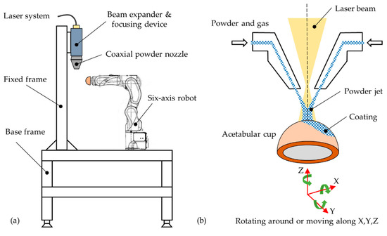
Figure 1.
(a) The laser cladding test bench. (b) Laser cladding coating on the acetabular cup.
The method proposed in this paper was implemented using processing software. Its architecture is shown in Figure 2. It mainly consisted of three modules: the CAD module, the path planning module and the simulation module. The CAD module offered two functions: graphic user interface for model handling and basic geometric operations for model transformation. The path planning module offered three functions: topological reconstruction of surface, cladding path planning and robot program generation. The simulation module was provided by the robot manufacturer.
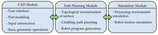
Figure 2.
The architecture of the processing software.
3. The Research Methods
The overall procedure of laser cladding path planning proposed in this paper is shown in Figure 3. The goal was to generate an optimal laser cladding path plan for the freeform surface parts of artificial joints. The overall procedure included mainly three steps:
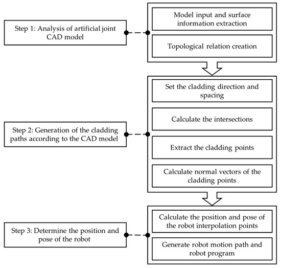
Figure 3.
The overall procedure.
Step 1: Analysis of artificial joint CAD model. The topological relation of the artificial joint surface was created by contacting feature vertices, edges and facets extracted from the artificial joint CAD model.
Step 2: Generation of the cladding paths according to the CAD model. The laser cladding path was automatically generated using the slicing algorithm based on a topological relation. The arch height error method was used to extract reasonable cladding points from a large number of intersections.
Step 3: Determination of the robot position and pose. The position and pose of the robot TCP were calculated according to the coordinates and normal vectors of the interpolation points. The robot motion paths were obtained by connecting the interpolation points sequentially, which finally were converted into the robot program.
4. Generation of Laser Cladding Paths
4.1. Topological Reconstruction of the Artificial Joint CAD Model
A STL (Stereo Lithography) file, which is a CAD data exchange file with a simple format, is very suitable for simulating, designing and modifying artificial joint models [20]. 3D models of artificial hip joints were converted into STL files by the CAD module, as shown in Figure 4a. Figure 4b shows the triangular facets in the STL file, which were described using three sets of X, Y and Z coordinates for each vertex and a normal unit vector indicating the direction of the facet. The three vertices were arranged counterclockwise. It must be mentioned that the triangular facets in the STL file were isolated and had no relation to the surrounding triangles. In other words, the STL file contained only graphical location information, not topological information. Therefore, in order to extract geometric information more effectively in the CAD model for subsequent path planning, it was necessary to pre-process STL files and create the relations among points, edges and facets [21]. In order to create the overall topological information at one time, the topology access should meet the following basic rules:
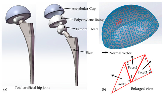
Figure 4.
(a) Main components of an artificial hip joint. (b) The triangular facets in an STL file of an acetabular cup.
- Rule 1: Given a triangular facet, get its three edges and three vertices.
- Rule 2: Given an edge, get its two adjacent triangular facets and two vertices.
- Rule 3: Given a vertex, get all triangular facets in which the vertex is located.
As shown in Figure 5, the respective data structures of vertices, edges and facets were designed according to the rules above. To store and read data more efficiently, three lists of vertices, edges and facets were created to store vertices, edges and facets respectively. The information of a vertex contained the index of the vertex, the coordinate of the vertex, the normal vector of the vertex and all indexes of the facet on which the vertex is located. The information of an edge contained the index of the edge, indexes of two end points of the edge and indexes of two facets on which the edge is located. The information of a facet contained the normal vector of the surface, the index of three vertices and the index of three edges.
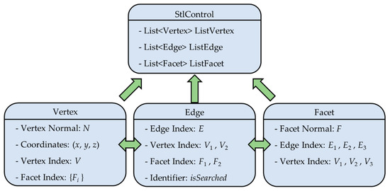
Figure 5.
The data structure after topology reconstruction.
According to the characteristics of the format of an STL file, a topological relation reconstruction algorithm was designed to read and parse STL files. The information of each triangular facet was read one by one, including the vertex coordinates and normal vector. Each vertex, edge and facet was topologically related to the surrounding elements and stored in the corresponding lists, as in the following steps.
Step 1: Read in the three vertices (V1, V2, V3) of a triangular facet in turn, and judge whether the vertex already exists in the list of vertices. If it does not exist, add it to the list of vertices; if it does, skip it.
Step 2: Read in the three edges (E1, E2, E3) of the current triangular facet in turn, and judge whether the edge already exists in the list of edges. If it does not exist, the index of the two vertices that make up the edge will be written in this edge, and add this edge to the list of edges; if it does, skip it.
Step 3: When all vertices and edges of a triangular facet (F) are added to the corresponding lists, the index of the three vertices and three edges that make up the facet will be written in this facet. Then, add this facet to the list of facets.
Step 4: Repeat Step 1–3 until all triangular facets are read and recorded.
To illustrate this procedure further, the pseudocode of this procedure is also given as the following Algorithm 1.
| Algorithm 1: Topological reconstruction algorithm. |
|
The local relations of a triangular mesh example extracted from the STL file are shown in Figure 6. The topological relation of edges after topological reconstruction and the quantity of the recorded data are listed in Table 1 and Table 2, respectively. Comparing Figure 6a with Figure 6b, it was obvious that the data structure was significantly simplified after topological reconstruction. The data of vertices, edges and facets were recorded uniquely after topological reconstruction, which contained no redundant information and provided complete topological relation. The topological relations of the edges are listed in Table 2. According to such information, it was easy to find the two vertices of each edge and the two facets on which the edge is located. This advantage played a huge role in the subsequent path planning method.
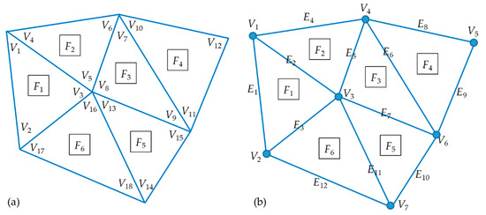
Figure 6.
The local relations schematic. (a) Before topological reconstruction, (b) after topological reconstruction.

Table 1.
Quantity of the recorded data.
Table 2.
Topology of edges after topological reconstruction.
4.2. Generation of the Laser Cladding Interpolation Points
4.2.1. The Slicing Algorithm Based on Topological Relation
In this section, the initial cladding path was generated from the CAD model based on the topological relations. A series of intersection point sets were obtained using a series of equidistant parallel planes intersecting the CAD model, which was called the slicing process. It was obvious that the process of intersection between the slicing planes and the CAD model was actually to find the intersection between the edges of the triangular facets and the cross planes. After all the intersection points were calculated, they were connected in a certain order to obtain the transversal lines.
In order to reduce the number of intersection calculations and avoid additional time consumption of sorting the intersection point sets, the slicing algorithm was designed based on topological relations of the edges. The core of the slicing algorithm was to constantly search the edge list for the edge that intersected with the current slicing plane and calculate the intersection point. The basic principle of the algorithm is, firstly, to traverse the list of edges to find an edge that intersects with the current slicing plane and, then, to search for next intersected edge in the adjacent edges of this edge according to the topological relation and to keep searching along the given direction until there are no intersected edges or return to the initial edge.
To distinguish the searched edge from the unsearched edge, a Boolean variable named isSearched was declared as an identifier in the data structure of the edge. The value of the identifier for all the edges was initially set as FALSE, which indicates none of the edges have been searched, and then changed to TRUE after being searched. The identifier was greatly useful for ensuring that each edge was accessed only once, which can significantly improve the efficiency of the slicing algorithm.
In addition, there were several important variables, namely the width, direction and range of the slicing process, which needed to be determined before the slicing algorithm was executed. The direction and width of the slicing process were specified by the user according to the specific laser cladding requirements. The range of the slicing process was determined by the maximum and minimum coordinates on the slicing direction in the list of vertices. When the slicing direction was determined, the slicing algorithm automatically calculated the range of the slicing process along the slicing direction.
Take the Z direction for example, the procedure of laser cladding path generation based on topological slicing is shown in Figure 7, where d is the slicing width, Z is the slicing direction and S is the value of the slicing plane in Z direction. The value of the slicing plane was initially set as the minimum value in Z direction and incremented by the value of the slicing width d. The slicing process started at the minimum coordinate and ended at the maximum coordinate.
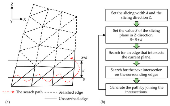
Figure 7.
(a) The topological slice process. (b) The cladding path generation in Z direction.
Each single transversal line was generated in the following steps:
Step 1: Find an edge that intersects with the current slicing plane but isSearched is FALSE. Figure out the intersection between this edge and the slicing plane and change isSearched of this edge to TRUE.
Step 2: Find all the adjacent edges of that edge according to the topological relationship between the points, edges and facets. If the isSearched of that edge is FALSE, figure out the intersection between that unsearched edge and the slicing plane; if it is TRUE, skip it.
Step 3: End the search when an unsearched edge cannot be found. Generate the path by joining all the intersections.
This slicing algorithm had two advantages. Firstly, through this method, it only needed to traverse the list of edges once to find the first edge intersecting the first current tangent plane. In the actual slicing process, only the edges contained in the triangular facet intersecting with the current tangent plane were searched and calculated, which greatly reduced the number of intersection calculations. Secondly, the topological slicing algorithm was automatically executed in a definite search direction. The ordered intersection sequence was directly obtained, which avoids the reordering and reconnection of the intersection set and greatly improves efficiency. In this way, the cladding path, which included a set of parallel, equidistant and directed transversal lines, was obtained directly.
To illustrate this procedure further, the pseudocode of this procedure is also given in Algorithm 2.
| Algorithm 2: Slicing algorithm based on topological relation. |
|
4.2.2. Simplification of the Intersection Data
It is difficult to directly interpolate curves when a curved surface part is processed using laser cladding. In engineering practice, the polyline, which includes multiple point-to-point line segments, is usually used to approximate the real curve line. The intersection points set directly obtained by the slicing algorithm was large and dense, which could not be directly used as the laser cladding processing point set. If it is directly used, the robot program file will be too large to execute, and the robot control system has to perform the interpolation point by point with extremely low efficiency. Furthermore, a greater degree of alloying and large dilution rate will occur during the laser cladding process when the cladding point set is too dense, which would pollute the composition of coatings and destroy its performance [22,23]. Therefore, on the premise of processing accuracy, it is essential to simplify the intersection point set and reasonably extract the effective processing points. The arch height error method [24] was introduced into this investigation as an effective mathematical method to optimize the discrete intersection point set.
The arch height calculation is shown in Figure 8. Known from the previous section, the set of discrete intersection points {Pi} was already an ordered sequence. The allowable arch height error dε was the key parameter that affected the number and density of the final interpolation point set, which determined the accuracy and quality of the final cladding path. In this study, dε was usually set as the allowable maximum limit value of defocusing change according to specific laser cladding requirements.
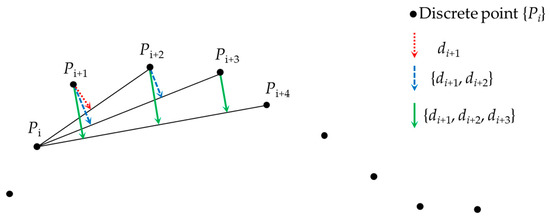
Figure 8.
Schematic diagram of arch height calculation.
The general steps for finding interpolation points are described as the following:
Step 1: Assuming that point Pi of the sequence is selected as the starting point, calculate the distance di+1 from the point Pi+1 to the line PiPi+2.
Step 2: If di+1 > dε, it means that the defocusing change exceeds the allowable range, then add Pi+1 as the valid interpolation point to the set of interpolation points. If di+1 < dε, it means that the defocusing change is within the allowable range, then go to the next step.
Step 3: Connect the Pi and Pi+3 points and calculate the distance from the points Pi+1 and Pi+2 to the line PiPi+3 as di+1 and di+2 respectively. The maximum dmax of the collection of {di+1, di+2} represents the maximum arch height of the arc segment PiPi+3. If dmax > dε, then add Pi+2 as the valid interpolation point to the set of interpolation points. If dmax < dε, continue to search forward until the maximum dmax of the collection of {di+1, di+2, di+3, … di+n} exceeds the allowable arch height error dε, then add the point Pi+n as the valid interpolation point to the set.
Step 4: Repeat Step 1-3, while point Pi+n is selected as the new starting point.
The simplification of the intersection point set usually started with the first point P1 in intersection points set {Pi} and ended with the last point Pm. Through the above method, all the effective processing interpolation points could be found and outputted as a sequence in the original order.
4.2.3. Calculation of the Normal Vector of Cladding Point
In order to facilitate the subsequent calculation of the position and pose of the robot TCP, the normal vector of vertex in the CAD model should be estimated first. The normal vector of each vertex was estimated by adding the normal vector of all triangles in which is located the center of gravity by area [25]. As shown in Figure 9, Aj denotes the area of the triangle, nj denotes the normal vector of each triangle, V denotes the common vertex, and N denotes the normal vector of the common vertex V. The normal vector N of vertex V can be estimated as follows:
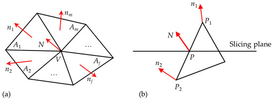
Figure 9.
(a) Vertex normal vector estimation. (b) Estimation of normal vector of the interpolation point.
This formula indicated that the normal vector of the triangle facet with a smaller area contributed more to the normal vector N of the common vertex V.
The normal vector of the processing interpolation point could be determined by the normal vectors of the two vertices on the edge, on which the interpolation point located. As shown in Figure 9b, P denotes an interpolation point, P1 and P2 denote two vertices on the edge containing P, and N, n1 and n2 denote the normal vectors of P, P1 and P2, respectively. The normal vector N of P could be calculated using the following equation:
where l1, l2 and l denote the length of the line segment P1P, PP2 and P1P2 respectively. If the slicing plane crossed exactly one vertex, then the normal vector N of P was equal to the normal vector of the vertex.
4.3. Determination of the Robot Position and Pose
In order to form a uniform and stable molten pool on the substrate during the laser cladding process, the laser beam is usually required to be perpendicular to the laser cladding surface. If the molten pool inclines during the cladding process, the shape and size of the coating section will be inconsistent, which affects the final quality of the coatings [26,27]. In this paper, therefore, the laser head was fixed on the worktable to keep it vertical all the time, and the workpiece clamped by the robot moved accordingly. In this mode, the laser beam was always perpendicular to the cladding surface, and the molten pool basically remained stable without tilting, which was beneficial for the formation of coatings.
The coordinates and normal vector of the interpolation point were recorded as V = [Vx Vy Vz]T and a = [ax ay az]T respectively in the workpiece coordinate system. The position and pose of the TCP defined as P = [Px Py Pz α β γ] could be calculated using a series of transformations. The rotation matrix T composed of vectors n, o and a could be expressed as:
where a = [ax ay az]T denotes the normal vector of the interpolation point, o = [ox oy oz]T is defined as the direction vector of the cladding processing path, and n = [nx ny nz]T is determined by n = o × a.
Matrix T represented the rotation matrix of the interpolation point relative to the workpiece coordinate system. However, in actual processing, the normal vector of the interpolation point was strictly required to coincide with the laser beam. Therefore, to meet this requirement, it was wise to set the interpolation point coordinate system {P} to be consistent with the world coordinate system {W} by adjusting the pose of the robot TCP. In other words, setting the pose of the robot made the vectors n, o and a coincide with the X, Y and Z axes of the world coordinate system, respectively, as shown in Figure 10.
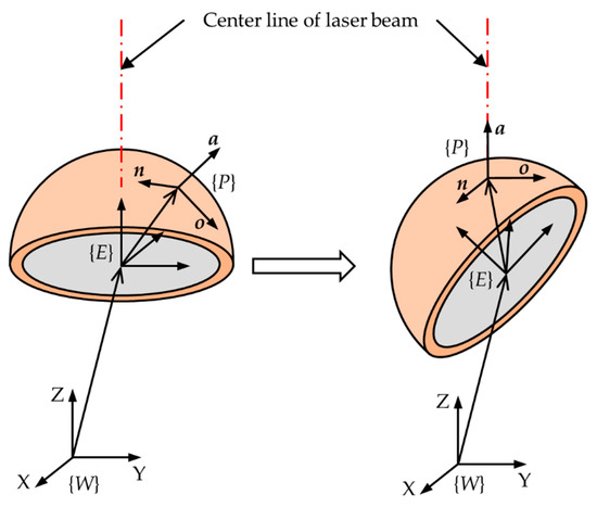
Figure 10.
Schematic diagram of robot TCP pose changes.
In this case, the rotation matrix T′ of the TCP coordinate system relative to the world coordinate system was equal to the rotation matrix of the workpiece coordinate system relative to the interpolation point coordinate system, expressed as the following:
As shown in Figure 11, vector L represents the position vector of the laser focus in the world coordinate system; vector V represents the position vector of the interpolation point in the workpiece coordinate system; and vector D represents the laser defocusing quantity of cladding processing. The position vector V' of the interpolation point in the world coordinate system could be expressed as the following:
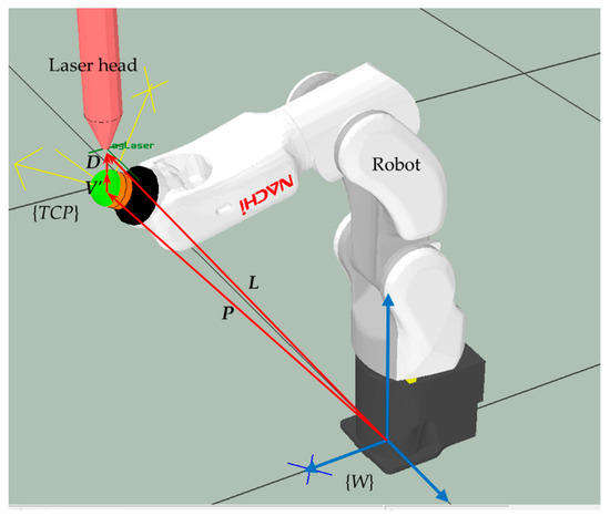
Figure 11.
Robot position and pose solution.
Furthermore, the position coordinates of the robot TCP could be expressed as the following:
The pose coordinates of the robot TCP are described as RPY rotation angles: α (Roll angle), β (Pitch angle) and γ (Yaw angle) as shown in Figure 12, which respectively represented the rotation of the robot TCP coordinate system around the Z, Y and X axis of the world coordinate system.
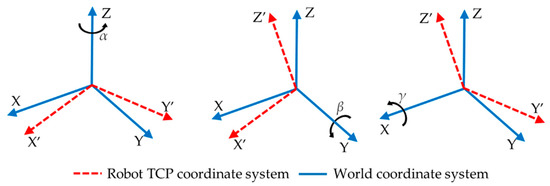
Figure 12.
RPY rotation angles: α (Roll angle), β (Pitch angle) and γ (Yaw angle).
The compound rotation matrix RPY was:
By comparing Equations (4) and (7), a set of equations for α, β and γ could be described:
By solving the equations, the expressions of α, β and γ could be obtained as follows:
According to the calculation results of Equations (6) and (9), the final position and pose of the robot TCP could be expressed as P = [Px Py Pz α β γ]. The robot positions and poses corresponding to all the interpolation points were obtained using the above method.
5. Experimental Validation
5.1. Automatic Path Generation Process
In order to realize the path planning method proposed in this paper, the authors developed a processing software based on C# and .net framework 4.5. The laser cladding path was generated and simulated using the processing software on a PC platform (CPU: Intel Core i3-4160 3.60 GHz; RAM 4.0 GB; OS: Microsoft Windows 10). An acetabular cup of an artificial hip joint with an outer diameter of 46 mm was selected as an example to verify the automatic generated path. The parameters related to path planning are listed in Table 3.
Table 3.
Parameters related to path generation.
The complete path generation process is shown in Figure 13. The STL model of the acetabular cup surface was sliced by five parallel planes in direction Z. Figure 13b shows five transversal lines with cladding spacing of 6 mm obtained by using the slicing algorithm based on a topological relation. Each single transversal line was connected by numerous intersection points in a laser scanning sequence. Figure 13c shows all the intersection points directly obtained. Figure 13d shows that the full path of the laser cladding consisted of five transversal lines end to end, each of which could be treated as single-pass cladding. To ensure the continuity of the cladding processing, the connecting lines were added between different single-pass cladding. When passing through the connecting lines, the robot moved without laser and powder. Figure 13e shows the direct result of the robot interpolation points with a defocus distance of 15 mm. Figure 13f shows the simplified result with an allowable arch height error of 0.5mm. Obviously, this not only guaranteed the shape precision of the surface machining, but also reduced the number of robot interpolations.
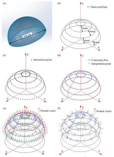
Figure 13.
Path generation process. (a) Acetabular cup STL model. (b) Transversal lines with cladding spacing at 6 mm. (c) All intersection points. (d) Full laser cladding path. (e) Direct result. (f) Simplified result with an allowable arch height error of 0.5mm.
Some key results of automatic path generation are listed in Table 4. Through topology reconstruction, the amount of data extracted and saved from the STL model was greatly reduced. The number of interpolation points were simplified from 850 to 74. The compression ratio of the interpolation points was approximately 8.7%, which contributed to reducing the size of the final robot program. On the other hand, the elapsed time of automatic path generation that involved software operations and computer processing was less than 30 seconds. When the full path was generated, the coordinates and normal vectors of the interpolation points were used to calculate the position and pose of the robot, which were finally transformed to the robot program.
Table 4.
Results of automatic path generation.
In the same case, the manual teaching method needed more than two hours to edit the processing program. Therefore, compared with the traditional manual teaching method, the automatic path generation method proposed in this paper had great advantages in saving time, improving efficiency and ensuring safety.
5.2. Simulation Experiment
The robot model is NACHI MZ04 from Japan and the simulation module named “FD on Desk” matches with the robot. As shown in Figure 14, after adding the entry and exit points, the text file was imported into the simulation module and compiled into the executable file of the robot program. First of all, the simulation environment was set up according to the actual working conditions. Then, the compiled robot program file was inputted into the simulation model to run in automatic operation mode.
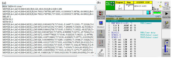
Figure 14.
(a) Text file of robot program. (b) The compiled robot program.
Some different positions and poses of the robot during the simulation process are shown in Figure 15. After the automatic operation started, the TCP of the robot moved from the original position to the entry point and then experienced each interpolation point one by one along the path. Finally, it went through the exit point and returned to the original position. The results showed that the TCP of the robot moved exactly along the planned interpolation path. Furthermore, in the whole simulation process, the robot achieved a complete and continuous movement without mechanical collision occurring or exceeding the range of motion. The relative position relationship between the laser beam and the surface of the acetabular cup was shown through different angles. During the laser cladding process, the laser beam was always vertical and perpendicular to the processed surface.
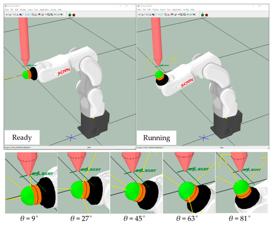
Figure 15.
Different positions and poses of robot during simulation process.
Figure 16 shows the changes of the robot pose angles during the simulation process. From those pictures, we can see the roll angle α changes from −180° to 180°, which indicates the robot TCP rotates around the X axis of the world coordinate system for circular motion, and the pitch angle β and the yaw angle γ changes from −90° to 90°, which indicates the robot TCP rotates around the Y and Z axis of world coordinate system in a half circular motion, respectively. The data results are consistent with the desired results of robot motion. The five cycles of smooth robot pose angles indicates that the robot TCP completes the whole motion correctly along the full path consisting of five parallel transversal lines. There are no singularities and drastic change of the robot pose in the motion process.
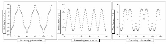
Figure 16.
Changes of robot pose angles (α, β, γ) during simulation process.
In a word, the simulation results preliminarily confirmed the correctness of the path automatically generated from the path planning module as well as the path planning method proposed in this paper.
6. Conclusions
In this paper, the laser cladding path planning for artificial joints was mainly investigated. In order to improve the efficiency of laser cladding on the surface of artificial joints, a path planning method for a laser cladding robot on an artificial joint surface based on topology reconstruction and a novel processing mode were designed. The main conclusions are as follows:
1. Different from traditional laser cladding mode, the presented mode of the laser beam fixation during workpiece movement met the requirements of the laser cladding process of the artificial joints and ensured the safety of the operator and equipment.
2. The path planning method based on the topological relations greatly reduced the amount of intersection calculation and directly obtained the sequential and simplified cladding path, which can be translated to the robot program with a small scale.
3. The planned path on the surface of a 46 mm artificial acetabular cup model was carried out by the simulation experiment. The results show that the robot accurately drove the artificial acetabular cup to move along the planned cladding path without mechanical collisions, trajectory deviations and so on.
Many facets of path planning remain for future investigation. We will still focus on the efficiency and quality of the path planning method. Moreover, we will combine laser cladding technology to investigate the quality of the coatings processed by applying the path planning method.
Author Contributions
Project administration, D.L.; software, Y.L.; supervision, T.C.; writing—original draft and editing, Y.L. All authors have read and agreed to the published version of the manuscript.
Funding
This work was supported by the National Natural Science Foundation of China, China (Grant 51775559), the Open Sharing Fund for Large-Scale Instruments and Equipment of Central South University, China (Grant CSUZC201919), and the Fund of the State Key Laboratory of High Performance Complex Manufacturing (Grant ZZYJKT2019-06).
Acknowledgments
The authors would like to thank the editors and reviewers for their helpful suggestions and comments, which indeed improved the manuscript.
Conflicts of Interest
The authors declare no conflict of interest.
References
- Kang, C.; Fang, F. State of the art of bioimplants manufacturing: Part I. Adv. Manuf. 2018, 6, 20–40. [Google Scholar] [CrossRef]
- Kang, C.; Fang, F. State of the art of bioimplants manufacturing: Part II. Adv. Manuf. 2018, 6, 137–154. [Google Scholar] [CrossRef]
- Pezzotti, G.; Yamamoto, K. Artificial hip joints: The biomaterials challenge. J. Mech. Behav. Biomed. 2014, 31, 3–20. [Google Scholar] [CrossRef] [PubMed]
- Goodman, S.B.; Barrena, E.G.; Takagi, M.; Konttinen, Y.T. Biocompatibility of total joint replacements: A review. J. Biomed. Mater. Res. A 2009, 90, 603–618. [Google Scholar] [CrossRef]
- Farid, M.M.; Hathout, R.M.; Fawzy, M.; Abou-Aisha, K. Fabrication of nano-structured calcium silicate coatings with enhanced stability, bioactivity and osteogenic and angiogenic activity. Colloids Surf. B Biointerfaces 2015, 126, 358–366. [Google Scholar] [CrossRef]
- Mattei, L.; di Puccio, F.; Piccigallo, B.; Ciulli, E. Lubrication and wear modelling of artificial hip joints: A review. Tribol. Int. 2011, 44, 532–549. [Google Scholar] [CrossRef]
- Chen, J.L.; Wang, D. Surface modification of titanium alloy with laser cladding RE oxides reinforced Ti3Al–matrix composites. Compos. Part B 2012, 43, 1207–1212. [Google Scholar] [CrossRef]
- Ghosh, S.; Abanteriba, S. Status of surface modification techniques for artificial hip implants. Sci. Technol. Adv. Mat. 2016, 17, 715–735. [Google Scholar] [CrossRef]
- Zhang, L.; Yuan, Z.; Tan, D.; Huang, Y. An Improved Abrasive Flow Processing Method for Complex Geometric Surfaces of Titanium Alloy Artificial Joints. Appl. Sci.-Basel 2018, 8, 1037. [Google Scholar] [CrossRef]
- Marzban, J.; Ghaseminejad, P.; Ahmadzadeh, M.H.; Teimouri, R. Experimental investigation and statistical optimization of laser surface cladding parameters. Int. J. Adv. Manuf. Technol. 2015, 76, 1163–1172. [Google Scholar] [CrossRef]
- Chen, F.W.; Yu, H. Research status of laser cladding on titanium and its alloys: A review. Mater. Des. 2014, 58, 412–425. [Google Scholar] [CrossRef]
- Baino, F.; Montealegre, M.A.; Orlygsson, G.; Novajra, G.; Vitale-Brovarone, C. Bioactive glass coatings fabricated by laser cladding on ceramic acetabular cups: A proof-of-concept study. J. Mater. Sci. 2017, 52, 9115–9128. [Google Scholar] [CrossRef]
- Shin, T.; Park, S.J.; Kang, K.S.; Kim, J.S.; Kim, Y.; Lim, Y.; Lim, D. A laser-aided direct metal tooling technology for artificial joint surface coating. Int. J. Precis. Eng. Manuf. 2017, 18, 233–238. [Google Scholar] [CrossRef]
- Tong, Y.; Zhong, M.; Li, J.; Li, D.; Wang, Y. Research on intelligent welding robot path optimization based on GA and PSO algorithms. IEEE Access 2018, 6, 65397–65404. [Google Scholar] [CrossRef]
- Funes-Lora, M.A.; Portilla-Flores, E.A.; Vega-Alvarado, E.; Blas, R.R.; Cruz, E.A.M.; Romero, M.F.C. A Novel Mesh Following Technique Based on a Non-Approximant Surface Reconstruction for Industrial Robotic Path Generation. IEEE Access 2019, 7, 22807–22817. [Google Scholar] [CrossRef]
- Zheng, H.; Cong, M.; Dong, H.; Liu, Y.; Liu, D. CAD-based automatic path generation and optimization for laser cladding robot in additive manufacturing. Int. J. Adv. Manuf. Technol. 2017, 92, 3605–3614. [Google Scholar] [CrossRef]
- Wang, X.; Sun, W.; Chen, Y.; Zhang, J.; Huang, Y.; Huang, H. Research on trajectory planning of complex curved surface parts by laser cladding remanufacturing. Int. J. Adv. Manuf. Technol. 2018, 96, 2397–2406. [Google Scholar] [CrossRef]
- Kluess, D.; Martin, H.; Mittelmeier, W.; Schmitz, K.; Bader, R. Influence of femoral head size on impingement, dislocation and stress distribution in total hip replacement. Med. Eng. Phys. 2007, 29, 465–471. [Google Scholar] [CrossRef]
- Phillips, A.T.; Pankaj; Usmani, A.S.; Howie, C.R. The effect of acetabular cup size on the short-term stability of revision hip arthroplasty: A finite element investigation. Proc. Inst. Mech. Eng. H 2004, 218, 239–249. [Google Scholar] [CrossRef]
- Ito, Y.; Nakahashi, K. Surface triangulation for polygonal models based on CAD data. Int. J. Numer. Methods Fluids 2002, 39, 75–96. [Google Scholar] [CrossRef]
- Xu, H.; Jing, W.; Li, M.; Li, W. A slicing model algorithm based on STL model for additive manufacturing processes. In Proceedings of the 2016 IEEE Advanced Information Management, Communicates, Electronic and Automation Control Conference (IMCEC), Xi’an, China, 3–5 October 2016; pp. 1607–1610. [Google Scholar]
- Salminen, J.P.; Kujanpää, V. Laser cladding with scanning optics: Effect of scanning frequency and laser beam power density on cladding process. J. Laser Appl. 2014, 26, 32002. [Google Scholar] [CrossRef]
- Lian, G.; Zhang, H.; Zhang, Y.; Huang, X.; Chen, C.; Jiang, J. Investigation of Geometric Characteristics in Curved Surface Laser Cladding with Curve Path. Metals 2019, 9, 947. [Google Scholar] [CrossRef]
- Tutunea-Fatan, H.L.R.; Feng, H. An improved tool path discretization method for five-axis sculptured surface machining. Int. J. Adv. Manuf. Technol. 2007, 33, 994–1000. [Google Scholar] [CrossRef]
- Sheng, W.; Xi, N.; Song, M.; Chen, Y.; MacNeille, P. Automated CAD-guided robot path planning for spray painting of compound surfaces. In Proceedings of the 2000 IEEE/RSJ International Conference on Intelligent Robots and Systems (IROS 2000) (Cat. No.00CH37113), Takamatsu, Japan, 31 October–5 November 2000; pp. 1918–1923. [Google Scholar]
- Lin, J.M.; Hwang, B.C. Coaxial laser cladding on an inclined substrate. Opt. Laser Technol. 1999, 31, 571–578. [Google Scholar] [CrossRef]
- Zhu, G.; Shi, S.; Fu, G.; Shi, J.; Yang, S.; Meng, W.; Jiang, F. The influence of the substrate-inclined angle on the section size of laser cladding layers based on robot with the inside-beam powder feeding. Int. J. Adv. Manuf. Technol. 2017, 88, 2163–2168. [Google Scholar] [CrossRef]


© 2020 by the authors. Licensee MDPI, Basel, Switzerland. This article is an open access article distributed under the terms and conditions of the Creative Commons Attribution (CC BY) license (http://creativecommons.org/licenses/by/4.0/).