Article

Detection and Monitoring of Bottom-Up Cracks in Road Pavement Using a Machine-Learning Approach

1
Department of Information, Infrastructure and Sustainable Energy (DIIES), Via Graziella, Feo di Vito, University Mediterranea of Reggio Calabria, 89124 Reggio Calabria, Italy
2
Faculty of Civil Engineering, Cracow University of Technology, Warszawska 24, 31155 Krakow, Poland
3
Institute for Software Systems in Technical Applications of Computer Science, University of Passau, Innstraße 43, D-94032 Passau, Germany
*
Author to whom correspondence should be addressed.
Algorithms 2020, 13(4), 81; https://doi.org/10.3390/a13040081
Submission received: 4 March 2020 / Revised: 27 March 2020 / Accepted: 30 March 2020 / Published: 31 March 2020
(This article belongs to the Special Issue Models and Technologies for Intelligent Transportation Systems)

Abstract

:
The current methods that aim at monitoring the structural health status (SHS) of road pavements allow detecting surface defects and failures. This notwithstanding, there is a lack of methods and systems that are able to identify concealed cracks (particularly, bottom-up cracks) and monitor their growth over time. For this reason, the objective of this study is to set up a supervised machine learning (ML)-based method for the identification and classification of the SHS of a differently cracked road pavement based on its vibro-acoustic signature. The method aims at collecting these signatures (using acoustic-sensors, located at the roadside) and classifying the pavement’s SHS through ML models. Different ML classifiers (i.e., multilayer perceptron, MLP, convolutional neural network, CNN, random forest classifier, RFC, and support vector classifier, SVC) were used and compared. Results show the possibility of associating with great accuracy (i.e., MLP = 91.8%, CNN = 95.6%, RFC = 91.0%, and SVC = 99.1%) a specific vibro-acoustic signature to a differently cracked road pavement. These results are encouraging and represent the bases for the application of the proposed method in real contexts, such as monitoring roads and bridges using wireless sensor networks, which is the target of future studies.

1. Introduction

Several types of distresses can lead to the failure of the flexible road pavements, which can be attributed to the following main causes [1,2,3,4]:
  • Inadequate mix design (e.g., excessive asphalt binder, or poor-quality asphalt binder, or aggregates);
  • Inadequate structural design (e.g., unsuitable road geometry, underestimated traffic load, insufficient layer thickness, and poor joint construction or location);
  • Inadequate construction quality (e.g., poor compaction and poor patching after utility cuts);
  • The increase in the traffic volume or of the number of vehicles with high axle loads;
  • Repeated traffic loading (fatigue);
  • Asphalt binder aging (i.e., oxidation of the binder resulting in a stiffer and more viscous material that is not able to hold the superficial aggregates that are pulled away by traffic);
  • Temperature (e.g., temperature cycling, freeze-thaw cycle, and low temperatures);
  • Moisture (e.g., excessive moisture in the subgrade);
  • Decreasing in pavement load supporting characteristics (i.e., loss in base, subbase or subgrade);
  • Reflective crack from an underlying layer (e.g., due to bottom-up cracking propagation, or presence of rigid objects);
  • Traffic start and stops;
  • Mechanical dislodging by uncommon traffic (e.g., studded tires, snowplow blades, or tracked vehicles);
  • Vibrations induced by the traffic, work zones, or natural events (e.g., earthquakes);
  • Maintenance policy pursued (e.g., failure- or condition-based).
Based on the main causes listed above, it is possible to state that: (1) they relate to intrinsic (e.g., inadequate design) or extrinsic (i.e., due to the interaction or the road pavement with the traffic or the environment); (2) the road pavement failures can be classified in surface and concealed; and (3) sometime surface failures are generated by concealed problems and/or failures.
Concealed failures (e.g., bottom-up cracks) are, by definition, difficult to be identified and localized. The methods that are commonly used to carry out this task have become unsustainable (i.e., destructive, spatially limited, and expensive), and obsolete (e.g., do not allow continuous monitoring, or are not able to provide real-time information). An infinite number of innovative solutions have been proposed in the last decades to perform the assessment and monitoring of the structural health conditions of road pavements. Furthermore, a big boost to this innovation can be attributed to the requests of the current and future smart cities [5], which sometimes come from the highest organization level, such as the Directive 2010/40/EU that strongly encourages the development of Intelligent Transportation System, ITS, to solve economic, energetic, environmental, social, and mobility-relate problems [6,7,8].

State of the Art about Technological Solutions Used to Detect Concealed Distresses in Road Pavements

Despite the noteworthy improvement of the Information and Communication Technologies (ICT), which is very well represented by the emerging field of the Internet of Things (IoT), it is still rare to find, in real contexts, monitoring systems based on ICT or IoT solutions that are able to detect and monitoring concealed distresses (e.g., bottom-up cracks). The current monitoring systems refer to mobile scanning technologies, such as those based on instrumented vehicles [9], unmanned aerial vehicles, airplanes, and satellites [10], ground penetrating radar [11], traffic speed deflectometer [12], smartphones’ accelerometers [13], and non-nuclear density gauges [14]. The main drawback of the above-mentioned technologies refers to the fact that they are focused on the recognition of surface distresses only, or on the derivation of these latter from surface-related parameters (e.g., texture and regularity [15], noise propagation [16], sound absorption [17], and vibration [18]).
Several approaches were used to process the data that come from the above mentioned solutions. Noteworthy examples applied for the structural health monitoring (SHM) of road pavements refer to (i) pothole detection using a fuzzy c-mean method based on morphological 2D image reconstruction [19], (ii) pavement roughness estimation based on analyses in the frequency domain [20], or the principal component analysis [21], or wavelet transform [22], (iii) automatic surface crack detection using wavelet-based analysis [23,24], (iv) crack detection using visual features extracted using Gabor filter [25], and particle filter [26], (v) surface crack detection using Otsu’s based method [27], (vi) surface crack classification by mean of support vector machine [28], (vii) use the fuzzy c-mean method to find the relationship between traffic emission (e.g., NOx) and the related built environment factors (e.g., short road in city center, bus stations density, ramps, and residential-commercial land proportion), and the relationship between built environment and the 24-hour congestion pattern [29,30], and (viii) ML-based approaches.
Among the different approaches listed above, those based on ML algorithms are becoming more and more popular because of the advantages offered by this approach. In particular, despite the ML algorithms requiring specialized skills for writing codes, a considerable computational effort, and big data sets (especially during their training), these algorithms are able to manage, automatically and in a smarter and easier way with respect to the more traditional techniques, the big data set mentioned above (e.g., sensor data, sounds, images, etc.), allowing detecting patterns and trends with good accuracy and in a wide range of applications. Consequently, a further analysis of the literature was carried out. Relevant and recent examples of the ML (and hybrid methods that consist of the combination of ML algorithms and the methods reported above) used to carry out the SHM of road pavements refer to (a) 3D reconstruction of concealed cracks using convolutional neural network (CNN)[31], (b) prediction of condition and performance, definition of management and maintenance strategies, surface distress forecasting (cracking, rutting, raveling, and roughness), structural evaluation (layer thicknesses, moduli, shear wave velocity, and deflection), distress identification using image analysis and classification, materials modeling [32], (c) detection of structural damage using wavelet-based and Artificial Neural Networks ANN [33,34], (d) detection of crack propagation using finite element method and ANN [35], (e) detection and classification of pavement crack using CNN and principal component analysis [36], (f) vision-based classification of cracks using a feed-forward ANN [37], and (g) predict the fracture energy of asphalt mixture specimens using an innovative ML algorithms [38].
In view of the foregoing, it is possible to assert that there is a lack in SHM methods based on ML-classifiers that aim at detecting and monitoring concealed cracks in road pavements. For this reason, in the study presented in this paper, a ML-based monitoring method that aims at detecting and classifying the concealed road cracks is proposed.
The remaining parts of the paper refer to: A) Section 2 (definition of the objectives of the study). B) Section 3, which refers to the description of the proposed method, to the experimental investigation carried out to gather the data set used in this study, and to the presentation of the different data analysis algorithms (i.e., a multilayer perceptron, a convolutional neural network, a random forest classifier, and a support vector classifier) used to analyze the data set mentioned above. C) Section 4, which refers to the presentation and discussions of the main results. D) Section 5 (Conclusions). E) References.

2. Objectives

The main objectives of the study presented in this paper were to (1) describe a new ML-based method specially designed for the SHM of road pavements, (2) describe the experimental investigation that was carried out to collect the acoustic signals (data set) used as input of the different classifiers presented in this study, and (3) define the most suitable classifier to process the data set collected during the experimental investigation.

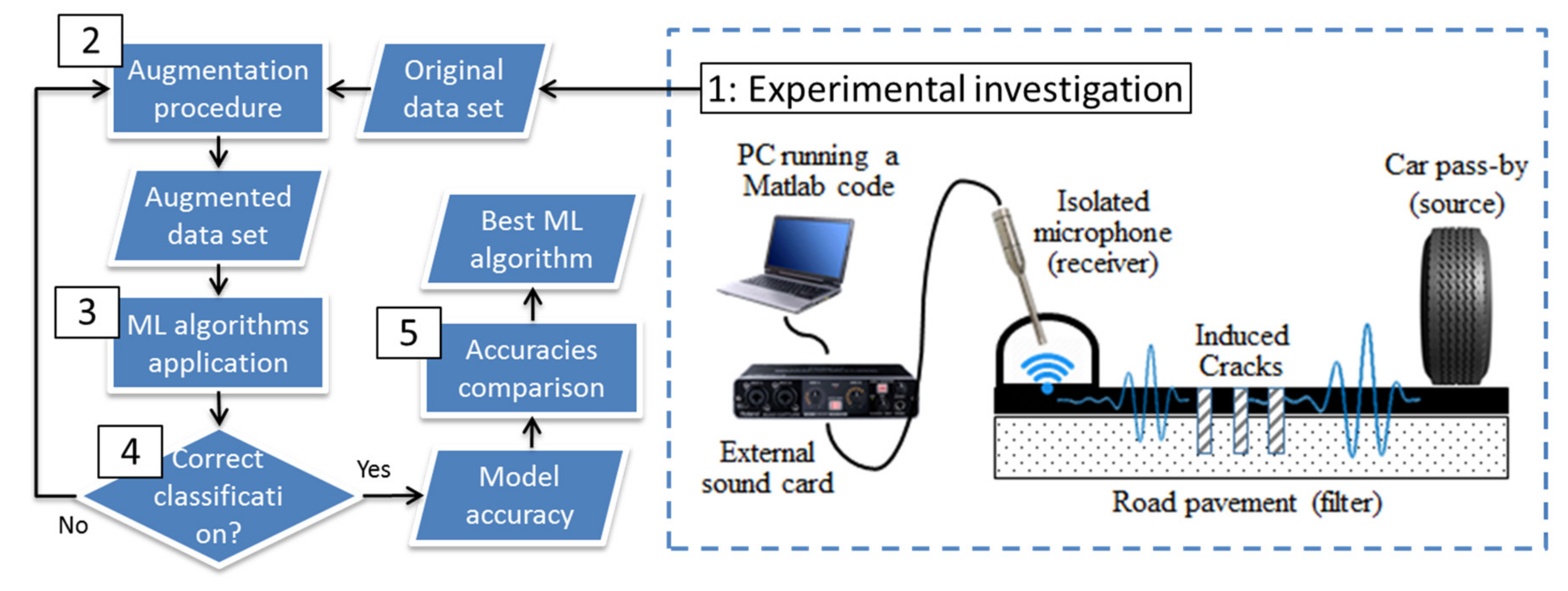
3. Innovative Method

3.1. The Method

The method considers the road pavement as a filter of the acoustic and seismic waves (see Figure 1) [39,40,41]. These latter are generated by a mechanical source (i.e., the vehicular traffic), travel into the medium (i.e., the road pavement), and finally are detected by a receiver (i.e., a microphone isolated from the airborne noise, attached on the road surface in a nondestructive way, connected to an external soundcard, in turn connected to a laptop running the Matlab code used to record sounds). Consequently, the related data set consists of the acoustic responses (ARs) of the road pavements to the loads induced by the vehicles. It is expected that the propagation of the above-mentioned signals will change if the structural health status (SHS) of the medium gets worse. As is well known, the seismic wave propagation depends on different parameters, such as the elastic modulus that in turns is affected by the temperature, the distance source–receiver (geometric damping), the material damping (related to the properties of the material and the vibration amplitude), the boundary conditions, and the occurrence of concealed distresses [42,43]. Figure 1 shows the tasks carried out in this study, from 1 (experimental investigation) to 5 (comparison of the results obtained by the ML algorithms, in terms of model accuracy, to find the best ML algorithm for the application of the proposed monitoring method).
Importantly, in the last years, a considerable effort was paid to set up the method. In particular, different experimental configurations and data analysis approaches were used to analyze the data gathered applying the proposed method. In particular, the analysis in time, frequency, and time–frequency domains, features extraction, hierarchical clustering [44], and Finite Element Models (FEM) [45] were used for the purposes mentioned above, while, in this study, different ML models were used. Based on the potentialities of the ML classifiers that were selected for this study and are presented in Section 3.3, good performance in term of automatic crack detection and monitoring was expected.

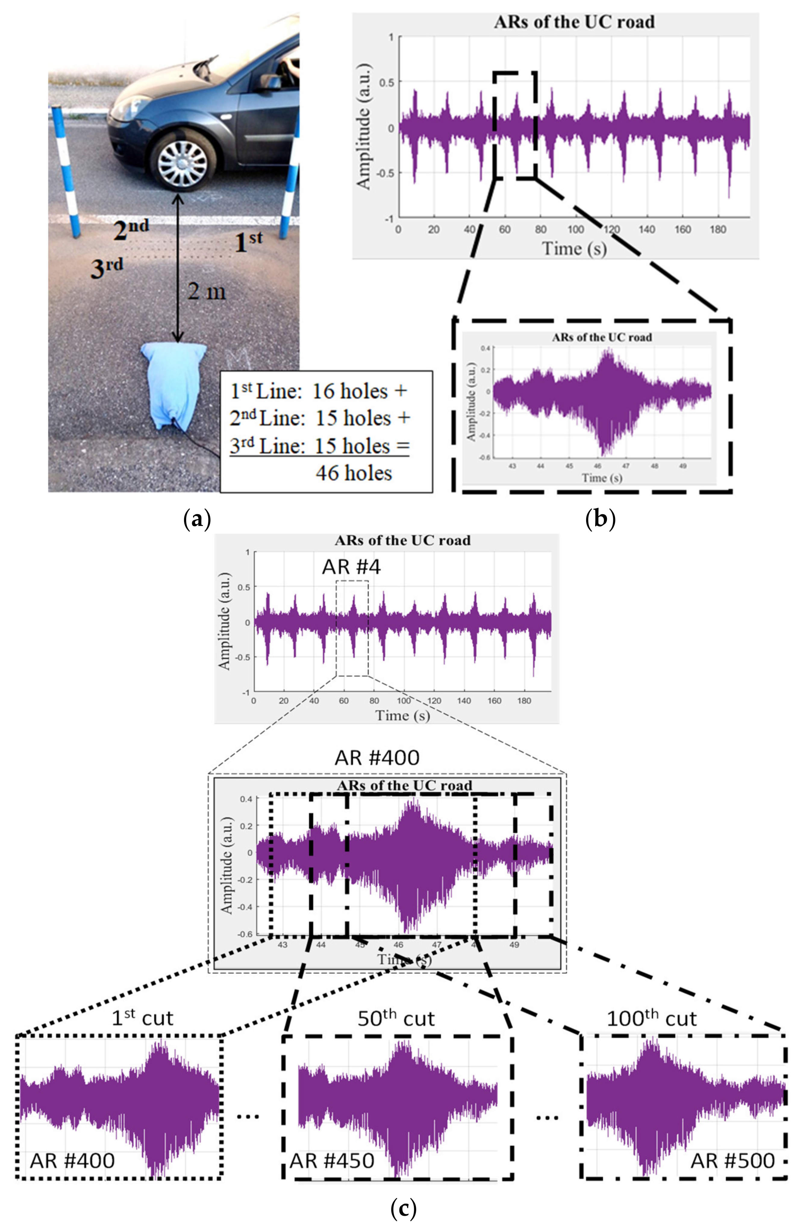
3.2. Experimental Investigation and Data Set Generation

This section aims at describing the experimental investigation that was carried out to collect the data set used to feed the different ML-classifiers.
The road pavement under investigation was a dense graded friction course (DGFC) consisting of two layers, i.e., one surface layer 3 cm-thick, and the second one 12 cm-thick. An accurate analysis of the surface of the road pavement used in this study allows recognizing the wheel paths. Therefore, we decided to pass the wheel of the car used during the tests over these areas. Importantly, no rutting phenomena (permanent deformations) or surface cracks were observed along the carriageway. Hence, even though the road was not new, it was considered suitable for our experiments.
Based on the well-known viscoelastic behavior of the material under test (i.e., asphalt concrete, which was also observed during previous experimental investigations), and with the aim of the proposed method (i.e., recognizing the occurrence of a damage from the vibro-acoustic response of the pavement), thermal excursions should be minimized, and other parameters, such as the speed of the vehicle, should be controlled or kept constant. To this end, the experimental investigation was carried out in one day, while the temperature of the pavement and the air were in the range 30-37 °C and 26-30 °C, respectively. At the same time, the speed of the vehicle used as a mechanical source was kept constant (about 20 km/h, i.e., the speed allowed in the parking area where the measurements were carried out).
The data set consisted of 40 ARs of a road pavement to the loads generated by 40 passages of a car (see Figure 2a), which was detected using the source of the system placed on the road surface 2 m far from the wheel path (i.e., the area of the pavement where the wheel of the vehicle is most likely to pass). The original data set (10 ARs for each SHSs of the pavement; see Figure 2b) was recorded running a Matlab code and using the highest sampling frequency allowed by the system, i.e., 192 kHz (to have signals with high resolution).
Based on a preliminary data analysis, it was observed that, because of the nature of the signal (pseudo-random) and of the high level of background noise due to the traffic and the environment, it was difficult to find the beginning of each acoustic response (AR). Consequently, we decided to use an augmentation procedure (see Figure 2c). The augmentation procedure was used several times in order to find the optimal data set size to properly classify the SHSs of the road pavement. In particular, each AR was cut several times using a window with a constant width, which was shifted with a constant step over the AR before the cut. After the augmentation, the augmented ARs were used as an input with different algorithms, using the Tensorflow and scikit-learn libraries [46,47].

3.3. The Machine Learning Classifiers Used

In this study, ANNs, random forest classifiers, and a set of support vector machine models were implemented in order to compare the efficiency of the developed ANN models.
As is well known [48], three practical issues must be faced in learning from samples: (1) capacity of the network (i.e., the number of patterns that can be stored, and the functions and the decision boundaries can be formed), (2) sample complexity (i.e., the number of training patterns needed to obtain a good generalization and avoid the “over-fitting”, namely obtaining good results in the training phase, and poor results in the test phase), and (3) computational complexity (i.e., the time required to estimate a solution from the training patterns). In more detail, the quality of the results of an ANN depends on the following variables, which should be carefully defined by the mean of trial-and-error approaches, and bearing in mind the following theoretical considerations and issues [49,50]: (i) data preprocessing (e.g., balancing an over- or underestimated class of signal, or enrichment using augmentation techniques such as scaling, translation, random noise addition, etc.) is recommended to accelerate the convergence of the testing results to the training results, (ii) input data set size (it should be sufficiently large to cover any variation in the problem domain), (iii) input data set partitioning (the percentages of signals of the data set used for learning and testing phases should be defined using the user experience, or the trial-and-error approach, or some statistical regression rule, (iv) learning rate (a high learning rate may lead to the overshooting of the optimal. This happens when the learning phase is too fast and the network is not able to carry out the classification, while a slow learning rate can make the network inefficient), (v) activation function (data non-linearity and noisiness should be considered before the selection of the activation function), (vi) hidden layers and node sizes (few hidden layers may underestimate complex patterns (under-parameterization), while too many hidden layers can lead the network to learn from the noise of the data (poor generalization). Furthermore, numerous hidden nodes may lead to time-consuming networks, while few hidden nodes can lead to the under-fitting of the network (network unable to obtain the underlying rules embedded in the data)), and (vii) training modes (weights updating) that refer to the size of the section of samples that are used in each testing iteration (i.e., the batch size). A trade-off between the batch size = 1 and the batch size = data set size should be found. If the batch size is equal to the data set size (a.k.a., batch training mode), a large storage for the weights is required, a better estimation of the error gradient can be obtained, but it is more likely that the network will be trapped in local minima. While, if a batch size = 1 is used (a.k.a., stochastic mode), an example-to-example training will be carried out, and this means smaller storage requirements for the weights, and fewer possibilities of entrapment in local minima. (viii) Convergence criteria or stopping criteria, namely the criteria used to stop the training, which can belong to the type “training error (i.e., error function ≤ small real number)”, “gradient error (i.e., gradient of the error function ≤ small real number)”, and “cross-validation (i.e., training the network using a part of the data set, and then validating the network using the remaining part of the data)”. Generally, during the training process the related error decreases when the number of nodes or training cycles increases. Examples of stopping criteria are the coefficient of determination and the sum of squared errors. Finally, confusion matrixes, or the hit (or miss) rate representing the percentage of examples classified correctly (or incorrectly) can be used as an error metric in classification problems, rather than the absolute deviation of the network classification from the target classification.
Based on the above, the following tasks were carried out: (a) the data set was preprocessed using the augmentation procedure described above in order to obtain an adequate input data set size (i.e., from an initial data set of 40 signals related to 4 SHSs, another 5 data sets were produced. The new data sets consist of 400, 800, 1600, 3200, and 4000 signals; see Table 1), (b) the data set was partitioned considering as a starting point the use of 50% of the ARs the training and the use of the remaining part (50%) for testing, (c) values extracted from an exponential scale starting from 0.001 (y = a × bx, where a = 0.001, and b = 2.5) were used as the learning rate, (d) the ReLu function was selected as activation function for the classification purpose (this activation function, f ( z ), is zero when z is less than zero, and it is equal to z when z is above or equal to zero, i.e., relu ( x ):=max ( 0, x)), and (e) the model accuracy (i.e., the ratio between the number of signals of the testing data set correctly classified and the total number of signals belonging to the testing data set to be classified), derived from confusion matrixes, were used to show the results of the classification. Furthermore, the Adadelta Optimized was selected as an optimizer function (for the adjustment of weights and biases).
ANNs are the basic classification approach considered in this study. The following ANN types were developed:
  • Multilayer perceptron (MLP);
  • Convolutional neural network (CNN).
The MLP consists of two fully connected hidden layers that are dedicated to the pattern recognition (using the ReLu as the activation function).
CNNs are commonly used for the classification of images (e.g., [31]), while, in this study, pseudorandom time series were used as input. These types of networks try to take advantage from the potentialities offered by the convolutional and pooling layers of the CNN (i.e., feature extraction and processing). The CNN used in this study consists of one convolution layer (feature extraction), one pooling layer (average pooling of the features extracted, applying the valid padding), and the same two fully connection layers used in the MLP (pattern recognition using the activation function ReLu). The activation function softmax cross entropy (i.e., measures the probability error in discrete classification tasks), and confusion matrixes were used to show and analyze the results of the classification.
In addition to ANNs, the following advanced ML-classifiers were developed:
  • Random forest classifier (RFC): an ensemble learning method for classification that operates by constructing a set of decision trees and returning the class that is the mode of the classes (classification) of the individual trees [38];
  • Support vector classifier (SVC): a supervised learning classifier with associated learning algorithms that can perform a nonlinear classification, implicitly mapping the model inputs into high-dimensional feature spaces.
The essential parameter of a RFC model is the number of estimators (the number of trees in the forest). The following types of SVC were implemented in the study:
  • SVC with linear kernel;
  • SVC with radial basis function (RBF) kernel;
  • SVC with polynomial kernel.
As it is stated in the scikit-learn documentation [47], two basic characteristics are used to parameterize SVC: (1) a kernel coefficient (gamma) and (2) the penalty parameter (C). The gamma parameter affects the influence of a single training example in the developed model. This parameter can be seen as the reciprocal of the radius of influence of samples selected by the model as support vectors. The penalty parameter C trades off correct classification of training examples against maximization of the decision function’s margin [46].

4. Results and Discussions

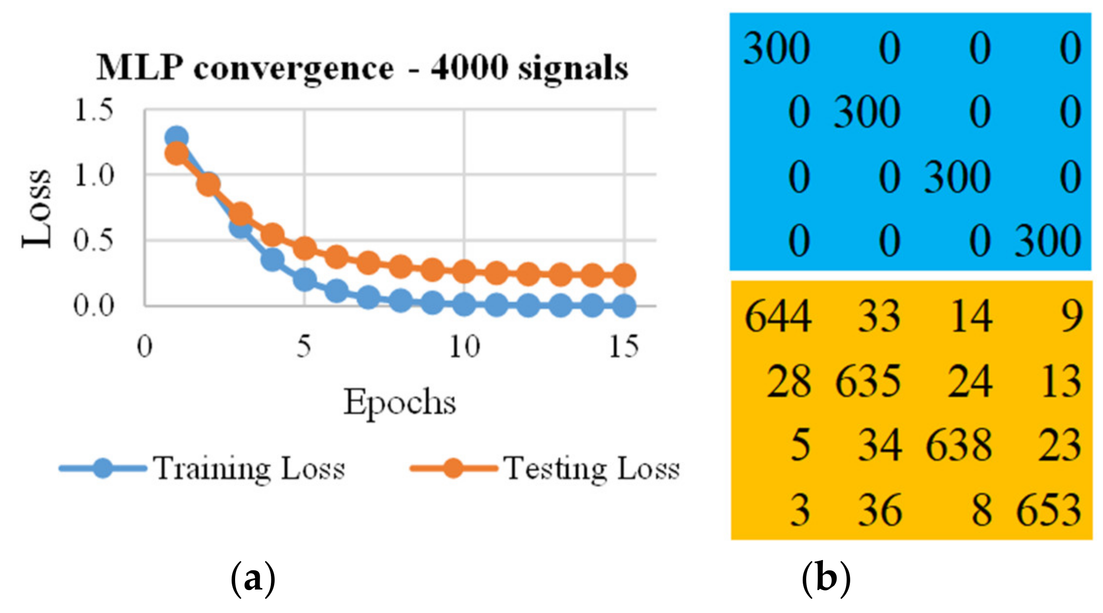
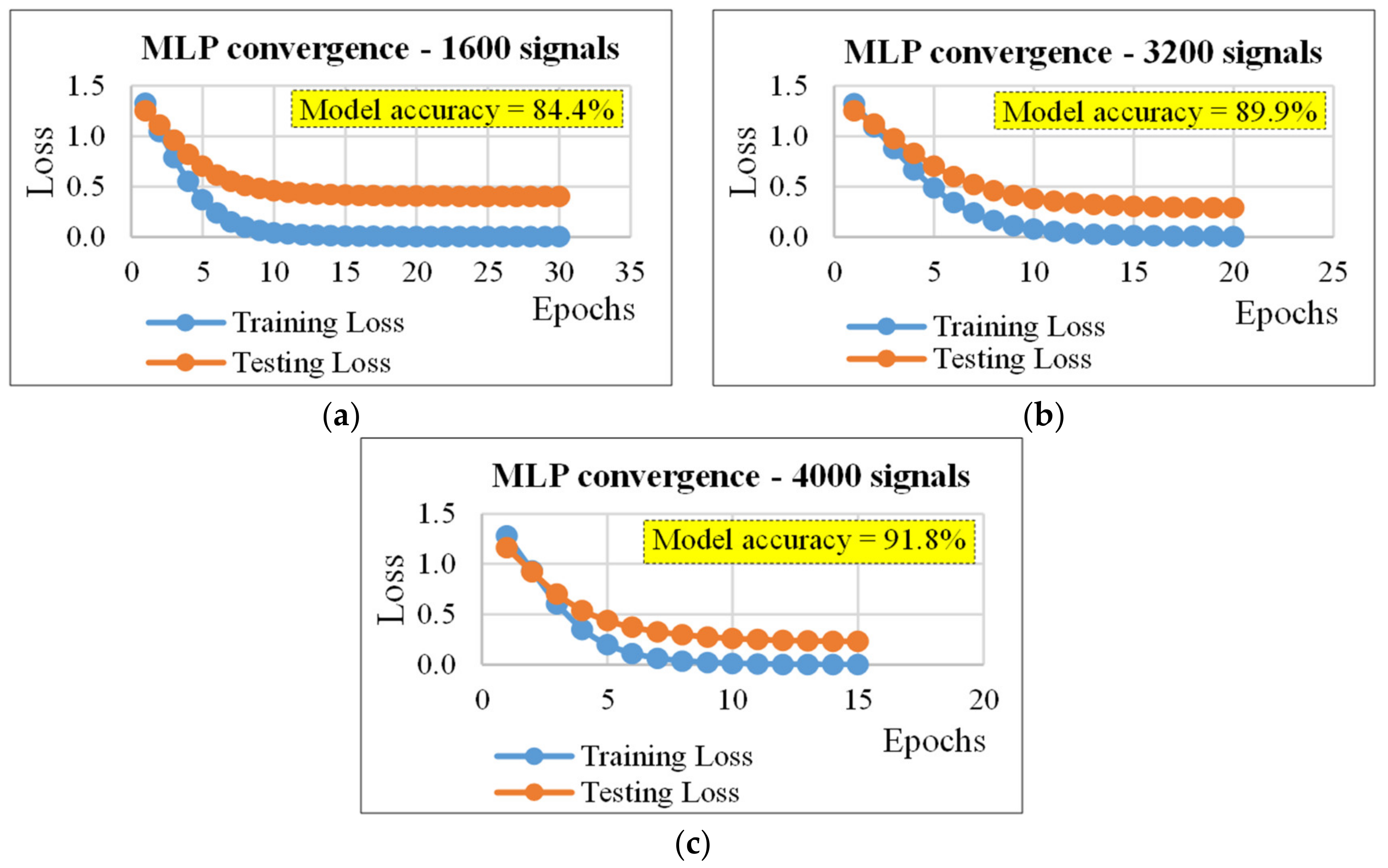
4.1. Multilayer Perceptron

The results of the classification procedure based on the MLP classifiers are presented in Table 1, where, for each data set size (D, first column), the following pieces of information were reported: (a) best data set partition (number of samples used in training versus testing processing); (b) number of nodes (nodes in each hidden layer); (c) number of epochs (number of times that the learning algorithm will work through the entire training dataset); (d) batch size (the training dataset is divided into more batches); and (e) model accuracy.
Figure 3 is an example of both graphical and numerical (confusion matrices) results that it is possible to obtain through the ML algorithms used in this study. In more detail, Figure 3a shows the trends of the training and testing losses during the epochs (e.g., 15) in which the algorithm (e.g., the MLP) works. Figure 3b shows the confusion matrix derived from (top) the training phase of the MLP algorithm, and (bottom) the testing phase. In more detail, a perfect training and a perfect testing (i.e. a perfect classification) were obtained when A) the losses tended to be zero when the epochs tended to be infinite and B) the non-zero elements of both the matrices mentioned above had all the non-zero elements in the main diagonal.
The results reported in Table 1 and Figure 4 point out how many signals were required to properly classify the SHS of a road pavement using the MLP. The results in Table 1 were derived in order to (i) minimize the use of signals for the training process, (ii) use few epochs that are a crucial factor when a real time monitoring is needed, (iii) have an overall reduction of the training loss (see Figure 3) of at least 65% (i.e., the difference between the highest, starting value and the lowest, final value), (iv) use a constant batch size of 16 samples, and (v) consider satisfying a model accuracy of at least 80%. Note that model accuracy is derived from the confusion matrixes of the training and testing processes. For example, by considering the results reported in the last row of Table 1 (recalled in Figure 3), the accuracy of 91.8% was derived dividing the sum of main diagonal elements of the confusion matrix of the testing phase (i.e., 644+635+638+653=2570; see Figure 3b bottom), with the training data set size (i.e., all the elements of the confusion matrix of the testing phase, which were 2800, and represented 70% of 4000).
Table 1 shows the best results obtained using the MLP. It is important to underline that, the MLP allows obtaining good results for the data sets with size greater than 800. It was not possible to reach the convergence of the model, which was measured considering a reduction of the training loss values (defined above) of 65% as lower limit. In addition, based on results, it can be stated that if the data set size increased (from 1600 to 4000), it is possible to (i) use a lower percentage of signals in the training phase (i.e., from 60% to 30%; see Table 1, column “Dataset partition”, rows 4th – 6th), (ii) speed-up the model by halving the epochs from 30 to 15 (see Table 1, column “# of epochs”), and (iii) obtain a better model accuracy (from 84.4% to 91.8% (see Table 1, last column)).

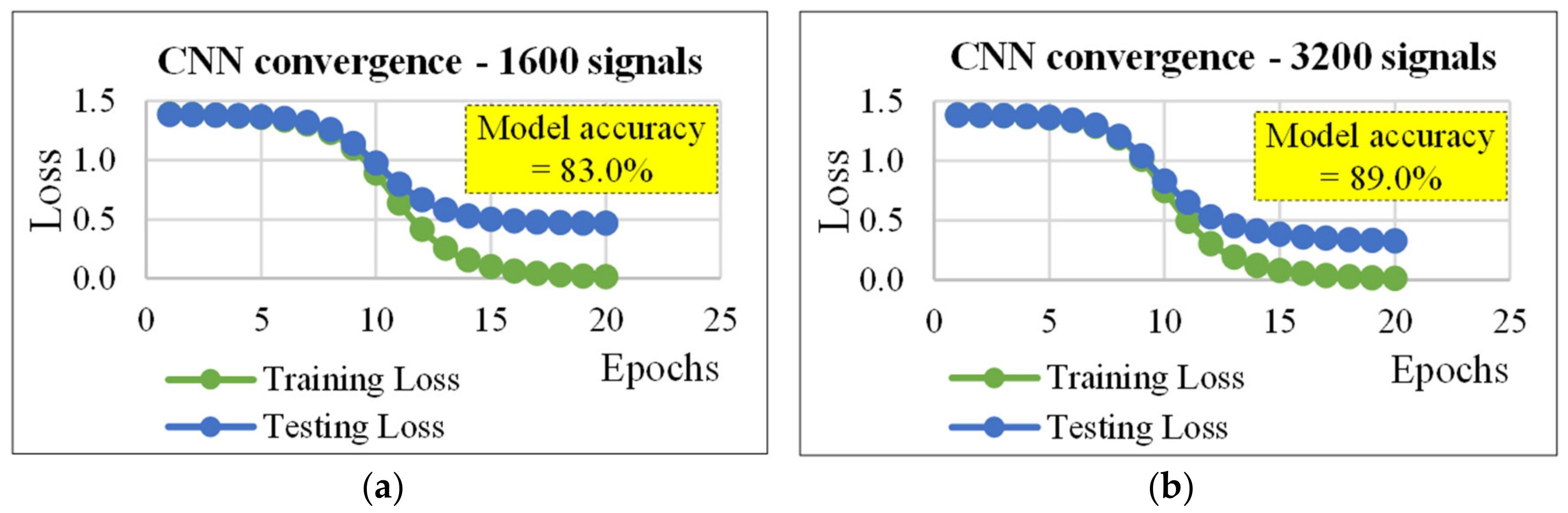
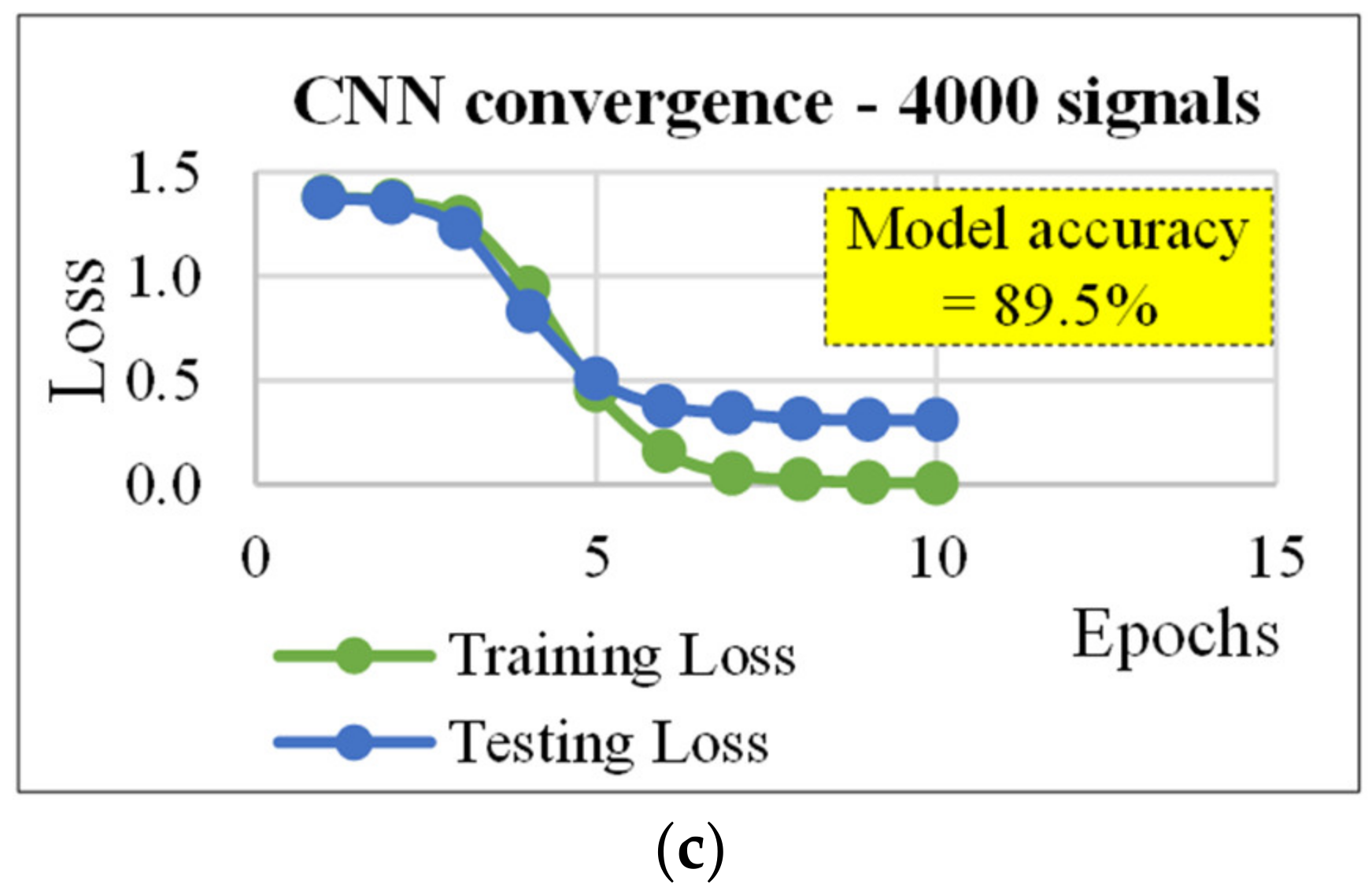
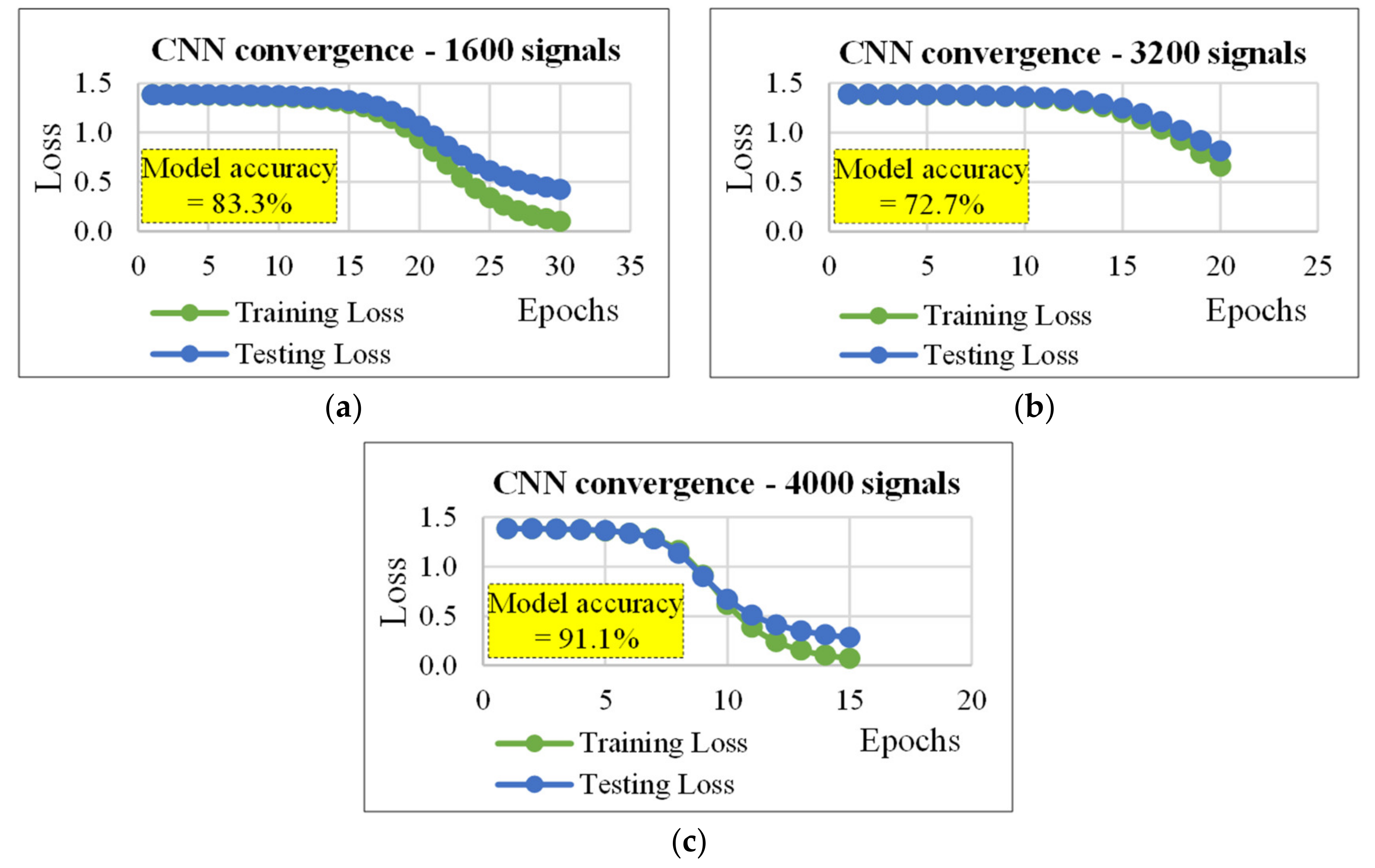
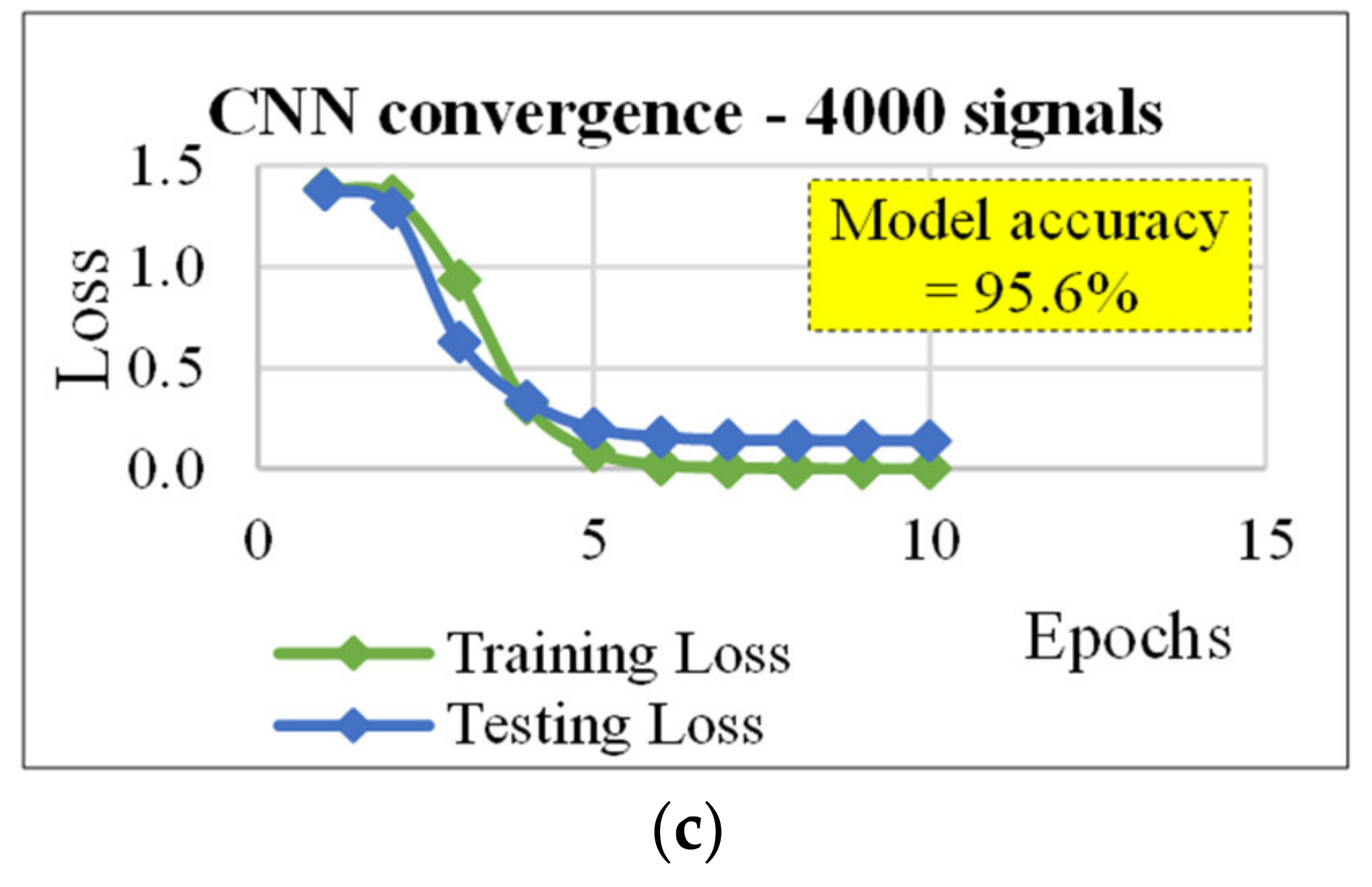
4.2. CNN for Classification

As for Table 1, Table 2 reports the parameters used in each layer of the CNN network and the results of its application on the same data sets used by the MLP. Note that, the batch size was the same used in the MLP (i.e., 16). Table 2 shows that, even if this network did not allow a good classification for data sets consisting of 40–800 ARs, the CNN allows obtaining results better than the MLP. In more detail, using the data set consisting of 1600 ARs a model accuracy of 89.5% can be reached under the following hypotheses: (1) 20 epochs; (2) 500 nodes per hidden layer; (3) a learning rate of 0.224; (4) a convolutional layer with 10 filters (length of the convolution window = 30; stride length of the convolution = 5); (5) a pooling layer with a window size equal to 10; and (6) a pool stride equal to 5 (the stride is the amount by which the filter shifts). The 89% of the data set (consisting of 3200 ARs) was properly classified using only the 30% of the ARs with the following parameters: 20 epochs, 700 nodes per hidden layer, a learning rate of 0.224, and the same convolutional and pooling layers used for the data set with 1600 signals. Finally, using the data set consisting of 4000 ARs, the 89.5% of data was properly classified. Figure 5, Figure 6 and Figure 7 refer to Table 2 and Table 3. In more detail, figures illustrate how the loss function used (error) is minimized when epochs increase.
It should be noted that, CNN allows obtaining the best results when the training data set consisted of 800 (for D = 1600, and D = 4000), or 960 ARs (for D = 3200). Importantly, if the configurations of the three cases (in terms of number of nodes and epochs) were compared, the case D = 4000 produced the best results using the simplest configuration. This key result could be due to the learning rate (=0.61) and the number of signals used for the training (=3200), which were both greater than those used in the other two configurations.
The next table shows the comparison between MLP and CNN, i.e., the results of the inclusion of a convolution layer and a pooling layer (with the same characteristics of those in Table 2) in the MLP (described in Section 4). Furthermore, it shows that increasing the number of filters (i.e., layers) in the convolutional layer it is possible to improve the accuracy.
By referring to the first two sections of Table 3, note that CNN had a lower accuracy than MLP.
By referring to the number of filters in the convolutional layer, note that results in Table 2 and Table 3 point out that different parameters were needed when applying the CNN to reach a higher model accuracy and particularly:
  • Bigger partitions of the data sets for the training (e.g., 30/70 as shown in the last row of Table 3, instead of 20/80 as reported in the last row of Table 2);
  • Higher number of filters (i.e., 100 and 150, as reported in the last section of Table 3, instead of 10, as shown in Table 2).
This allows CNN to reach a higher model accuracy (e.g., 95.6% instead of 91.8 for the data set consisting in 4000 ARs) and to get accuracies higher than MLP ones.

4.3. Random Forest Classifier

The RFCs, implemented with the help of the scikit-learn predefined class, were trained with the prepared data. The complexity of the classifiers was varied on the basis of the number of used estimators. The set of 5, 10, 20, 50, and 100 estimators (decision trees) shaping the random forest was considered in the experiment. Additionally, different proportions of the training and testing sets were used for the fitting of the RFC parameters and in order to estimate model accuracy. The parameters of the RFCs implemented with the highest accuracy are presented in Table 4.

4.4. Support Vector Classifier

After the first stage of the simulations with different types of SVCs, models with linear and polynomial kernels were excluded from the experiment due to their low accuracy compared to models with the RBF kernel. The kernel coefficients were varied from 0.012 to 0.018 with the step of 0.002. Results of the experiment obtained through the best SVC are shown in Table 5.
Results indicate that the use of the SVC described above, with properly fitted parameters, allows obtaining a classification accuracy even higher than the one of ANN models.

5. Conclusions

Results show the possibility of associating a specific vibro-acoustic signature to a road pavement through the efficient ML-classifier.
The efficiency of the classifiers used was evaluated in terms of model accuracy derived from confusion matrixes.
In order to obtain models suitable for the application described in this paper, trade-off solutions were found acting principally on the number of nodes of the hidden layers, the learning rate, the number of epochs, and the number of filters of the convolution layer.
In particular, the number of epochs was considered a key factor to obtain faster ANNs. The ANNs used (MLP and CNN) were able to classify data sets consisting of a number of signals greater than 800, with accuracies that range from 83% to 95.4%. Importantly, the CNN includes the MLP and allows obtaining better results (i.e., MLP = 91.8% while CNN = 95.6%). In more detail, the CNN allows using smaller signals for the training, and when the same data partitions were used, the CNN was able to obtain model accuracies greater than for MLP.
Random forest classifiers (RFCs) as an alternative to ANNs could produce results comparable with MLPs (i.e., MLP = 91.8% while RFC = 91.0%) but somehow worse than CNN models with the parameters optimized. However, experiments show that SVM models could produce a better classification accuracy (99.1%) for the problem considered in this paper.
These results were encouraging and represent the bases for the application of the proposed SHM method in real contexts by the mean of suitable and well-designed tools for intelligent transportation systems. Possible applications of the proposed method include the monitoring of structural health status of several types of assets, such as road pavements, bridges, buildings, etc. using for example a wireless sensor network consisting of sensor nodes located (i.e., non-destructive test method) beside the carriageway.
Future studies will focus on crucial topics related to the field of the asset monitoring, such as: (1) Investigate the effect of different types of distresses on the vibro-acoustic signatures of the different road pavements in different environmental, boundary, and structural conditions (i.e., considering (a) daily, seasonal, and annual changes, (b) different thickness and composition of the road pavement layers, and (c) different distresses, respectively). (2) Include more sensors (e.g., temperature and humidity sensors, gas and smoke concentration sensors, and accelerometers. This task was partially addressed in [51,52]) to gather also environmental data (e.g., unusual temperatures, presence of water, particulate matters, etc.), traffic-related data (e.g., traffic flow, noise level, congestion level, etc.), and emergency-related data (e.g., occurrence of a car accident, presence of fire, smoke, etc.).

Author Contributions

Conceptualization, F.G.P., R.F., V.N. and T.S.; Methodology, F.G.P., R.F., V.N. and T.S.; Investigation, F.G.P., R.F., V.N. and T.S.; Data Curation, F.G.P., R.F., V.N. and T.S.; Writing—Review and Editing, F.G.P., R.F., V.N. and T.S. All authors have read and agreed to the published version of the manuscript.

Funding

This research was funded by the Italian Research Project - PRIN: PROGETTI DI RICERCA DI RILEVANTE INTERESSE NAZIONALE—Bando 2017—Prot. 2017XYM8KC “Urban safety, sustainability, and resilience: 3 paving solutions, 4 sets of modules, 2 platforms.” Acronym: USR342.

Acknowledgments

Authors want to express their gratitude to Ruben Fischer (researcher at the FORWISS institute, University of Passau, Germany) and to Mariantonia Cotronei (professor at the University of Reggio Calabria, DIIES department) for their suggestions.

Conflicts of Interest

The authors declare no conflict of interest.

References

  1. Moghaddam, T.B.; Karim, M.R.; Abdelaziz, M. A review on fatigue and rutting performance of asphalt mixes. Sci. Res. Essays 2011, 6, 670–682. [Google Scholar]
  2. Gedafa, D.S. Performance Prediction and Maintenance of Flexible Pavement. In Proceedings of the 2007 Mid-Continent Transportation Research Symposium, Ames, IA, USA, 16 August 2007; pp. 16–17. [Google Scholar]
  3. Lekei, E.E.; Ngowi, A.V.; London, L. Undereporting of Acute Pesticide Poisoning in Tanzania: Modelling Results from Two Cross-Sectional Studies. Environ. Health 2016, 15, 18. [Google Scholar] [CrossRef] [Green Version]
  4. Celauro, C.; Praticò, F.G. Asphalt mixtures modified with basalt fibres for surface courses. Constr. Build. Mater. 2018, 170, 245–253. [Google Scholar] [CrossRef]
  5. Pop, M.-D.; Proștean, O. A comparison between smart city approaches in road traffic management. Procedia Soc. Behav. Sci. 2018, 238, 29–36. [Google Scholar] [CrossRef]
  6. The European Parliament and the Council of the European Union. Directive 2010/40/EU of the European Parliament and of the Council of 7 July 2010 on the framework for the deployment of Intelligent Transport Systems in the field of road transport and for interfaces with other modes of transport (Text with EEA relevance). 2010. Available online: https://www.cita.lu/uploads/its/Directive_2010-40-EU_EN.pdf (accessed on 20 January 2020).
  7. Praticò, F.G.; Moro, A.; Ammendola, R. Potential of fire extinguisher powder as a filler in bituminous mixes. J. Hazard. Mater. 2010, 173, 605–613. [Google Scholar] [CrossRef] [PubMed]
  8. Praticò, F.G.; Vaiana, R.; Gallelli, V. Transport and Traffic Management by Micro Simulation Models: Operational Use and Performance of Roundabouts; WIT Transactions on the Built Environment: Southampton, UK, 2012; Volume 128, pp. 383–394. [Google Scholar]
  9. Cafiso, S.; D’Agostino, C.; Delfino, E.; Montella, A. From manual to automatic pavement distress detection and classification. In Proceedings of the 5th IEEE International Conference on Models and Technologies for Intelligent Transportation Systems (MT-ITS), Naples, Italy, 26–28 June 2017; pp. 433–438. [Google Scholar]
  10. Schnebele, E.; Tanyu, B.F.; Cervone, G.; Waters, N. Review of remote sensing methodologies for pavement management and assessment. Eur. Transp. Res. Rev. 2015, 7, 1–19. [Google Scholar] [CrossRef] [Green Version]
  11. Benedetto, A.; Tosti, F.; Bianchini Ciampoli, L.; D’Amico, F. An overview of ground-penetrating radar signal processing techniques for road inspections. Signal Process. 2017, 132, 201–209. [Google Scholar] [CrossRef]
  12. Katicha, S.W.; Flintsch, G.; Bryce, J.; Ferne, B. Wavelet denoising of TSD deflection slope measurements for improved pavement structural evaluation. Comput. Civ. Infrastruct. Eng. 2014, 29, 399–415. [Google Scholar] [CrossRef]
  13. Carlos, M.R.; Aragon, M.E.; Gonzalez, L.C.; Escalante, H.J.; Martinez, F. Evaluation of detection approaches for road anomalies based on accelerometer readings - Addressing who’s who. IEEE Trans. Intell. Transp. Syst. 2018, 19, 3334–3343. [Google Scholar] [CrossRef]
  14. Praticó, F.G.; Moro, A.; Ammendola, R. Factors affecting variance and bias of non-nuclear density gauges for porous european mixes and dense-graded friction courses. Balt. J. Road Bridg. Eng. 2009, 4, 99–107. [Google Scholar] [CrossRef]
  15. Praticò, F.G.; Vaiana, R. A study on the relationship between mean texture depth and mean profile depth of asphalt pavements. Constr. Build. Mater. 2015, 101, 72–79. [Google Scholar] [CrossRef]
  16. Licitra, G.; Teti, L.; Cerchiai, M. A modified Close Proximity method to evaluate the time trends of road pavements acoustical performances. Appl. Acoust. 2014, 76, 169–179. [Google Scholar] [CrossRef]
  17. Morgan, P.A.; Watts, G.R. A novel approach to the acoustic characterisation of porous road surfaces. Appl. Acoust. 2003, 64, 1171–1186. [Google Scholar] [CrossRef]
  18. Lak, M.A.; Degrande, G.; Lombaert, G. The effect of road unevenness on the dynamic vehicle response and ground-borne vibrations due to road traffic. Soil Dyn. Earthq. Eng. 2011, 31, 1357–1377. [Google Scholar] [CrossRef]
  19. Ouma, Y.O.; Hahn, M. Pothole detection on asphalt pavements from 2D-colour pothole images using fuzzy c-means clustering and morphological reconstruction. Autom. Constr. 2017, 83, 196–211. [Google Scholar] [CrossRef]
  20. Barbosa, R.S. Vehicle dynamic response due to pavement roughness. J. Braz. Soc. Mech. Sci. Eng. 2011, 33, 302–307. [Google Scholar] [CrossRef] [Green Version]
  21. Zhang, Y.; McDaniel, J.G.; Wang, M.L. Estimation of pavement macrotexture by principal component analysis of acoustic measurements. J. Transp. Eng. 2014, 140, 1–11. [Google Scholar] [CrossRef]
  22. Zelelew, H.M.; Papagiannakis, A.T.; De León Izeppi, E.D. Pavement macro-texture analysis using wavelets. Int. J. Pavement Eng. 2013, 14, 725–735. [Google Scholar] [CrossRef]
  23. Subirats, P.; Dumoulin, J.; Legeay, V.; Barba, D. Automation of pavement surface crack detection using the continuous wavelet transform. In Proceedings of the International Conference on Image Processing, Atlanta, GA, USA, 8–11 October 2006; pp. 3037–3040. [Google Scholar]
  24. Ouma, Y.O.; Hahn, M. Wavelet-morphology based detection of incipient linear cracks in asphalt pavements from RGB camera imagery and classification using circular Radon transform. Adv. Eng. Inform. 2016, 30, 481–499. [Google Scholar] [CrossRef]
  25. Zalama, E.; Gómez-García-Bermejo, J.; Medina, R.; Llamas, J. Road crack detection using visual features extracted by gabor filters. Comput. Civ. Infrastruct. Eng. 2014, 29, 342–358. [Google Scholar] [CrossRef]
  26. Hassan, N.; Mathavan, S.; Kamal, K. Road crack detection using the particle filter. In Proceedings of the 23rd IEEE International Conference on Automation and Computing (ICAC), Huddersfield, UK, 7–8 September 2017. [Google Scholar]
  27. Sitara, S.N. Review and analysis of crack detection and classification techniques based on crack types. Int. J. Appl. Eng. Res. 2018, 13, 6056–6062. [Google Scholar]
  28. Moussa, G.; Hussain, K. A new technique for automatic detection and parameters estimation of pavement crack. In Proceedings of the 4th International Multi-Conference on Engineering and Technological Innovation, Orlando, FL, USA, 19 July 2011; Volume 2, pp. 11–16. [Google Scholar]
  29. Sun, D.; Zhang, K.; Shen, S. Analyzing spatiotemporal traffic line source emissions based on massive didi online car-hailing service data. Transp. Res. Part D Transp. Environ. 2018, 62, 699–714. [Google Scholar] [CrossRef]
  30. Zhang, K.; Sun, D.J.; Shen, S.; Zhu, Y. Analyzing spatiotemporal congestion pattern on urban roads based on taxi GPS data. J. Transp. Land Use 2017, 10, 675–694. [Google Scholar] [CrossRef]
  31. Tong, Z.; Gao, J.; Zhang, H. Recognition, location, measurement, and 3D reconstruction of concealed cracks using convolutional neural networks. Constr. Build. Mater. 2017, 146, 775–787. [Google Scholar] [CrossRef]
  32. El-Basyouny, M.; Jeong, M.G. Prediction of the MEPDG asphalt concrete permanent deformation using closed form solution. Int. J. Pavement Res. Technol. 2014, 7, 397–404. [Google Scholar]
  33. Moghadas Nejad, F.; Zakeri, H. An expert system based on wavelet transform and radon neural network for pavement distress classification. Expert Syst. Appl. 2011, 38, 7088–7101. [Google Scholar] [CrossRef]
  34. Shi, A.; Yu, X.H. Structural damage detection using artificial neural networks and wavelet transform. In Proceedings of the IEEE International Conference on Computational Intelligence for Measurement Systems and Applications (CIMSA), Tianjin, China, 2–4 July 2012; pp. 7–11. [Google Scholar]
  35. Gajewski, J.; Sadowski, T. Sensitivity analysis of crack propagation in pavement bituminous layered structures using a hybrid system integrating Artificial Neural Networks and Finite Element Method. Comput. Mater. Sci. 2014, 82, 114–117. [Google Scholar] [CrossRef]
  36. Wang, X.; Hu, Z. Grid-based pavement crack analysis using deep learning. In Proceedings of the 4th International Conference on Transportation Information and Safety (ICTIS), Banff, AB, Canada, 8–10 August 2017; pp. 917–924. [Google Scholar]
  37. Mokhtari, S.; Wu, L.; Yun, H.B. Comparison of supervised classifcation techniques for vision-based pavement crack detection. Transp. Res. Rec. 2016, 2595, 119–127. [Google Scholar] [CrossRef]
  38. Majidifard, H.; Jahangiri, B.; Buttlar, W.G.; Alavi, A.H. New machine learning-based prediction models for fracture energy of asphalt mixtures. Meas. J. Int. Meas. Confed. 2019, 135, 438–451. [Google Scholar] [CrossRef]
  39. Fedele, R.; Praticò, F.G.; Carotenuto, R.; Della Corte, F.G. Energy savings in transportation: Setting up an innovative SHM method. Math. Model. Eng. Probl. 2018, 5, 323–330. [Google Scholar] [CrossRef]
  40. Fedele, R.; Praticò, F.G.; Carotenuto, R.; Della Corte, F.G. Damage detection into road pavements through acoustic signature analysis: First results. In Proceedings of the 24th International Congress on Sound and Vibration (ICSV), London, UK, 23–27 July 2017. [Google Scholar]
  41. Fedele, R.; Della Corte, F.G.; Carotenuto, R.; Praticò, F.G. Sensing road pavement health status through acoustic signals analysis. In Proceedings of the 13th Conference on PhD Research in Microelectronics and Electronics (PRIME), Giardini Naxos, Italy, 12–15 June 2017; pp. 165–168. [Google Scholar]
  42. Nguyen, S.T.; To, Q.D.; Vu, M.N. Extended analytical solutions for effective elastic moduli of cracked porous media. J. Appl. Geophys. 2017, 140, 34–41. [Google Scholar] [CrossRef]
  43. Kim, D.S.; Lee, J.S. Propagation and attenuation characteristics of various ground vibrations. Soil Dyn. Earthq. Eng. 2000, 19, 115–126. [Google Scholar] [CrossRef]
  44. Fedele, R.; Praticò, F.G. Monitoring infrastructure asset through its acoustic signature. In Proceedings of the INTER-NOISE and NOISE-CON Congress and Conference Proceedings, Madrid, Spain, 30 September 2019. [Google Scholar]
  45. Fedele, R.; Praticò, F.G.; Pellicano, G. The prediction of road cracks through acoustic signature: Extended finite element modeling and experiments. J. Test. Eval. 2021, 49, 2230–2237. [Google Scholar] [CrossRef]
  46. Google Brain Tensorflow. Available online: https://www.tensorflow.org/tutorials/ (accessed on 20 January 2020).
  47. Cournapeau, D. Scikit-Learn. Available online: https://scikit-learn.org/stable/ (accessed on 20 January 2020).
  48. Jain, A.K.; Mao, J.; Mohiuddin, K.M. Artificial neural networks: A tutorial. Computer 1996, 29, 31–44. [Google Scholar] [CrossRef] [Green Version]
  49. Basheer, I.A.; Hajmeer, M. Artificial neural networks: Fundamentals, computing, design, and application. J. Microbiol. Methods 2000, 43, 3–31. [Google Scholar] [CrossRef]
  50. Praticò, F.G. On the dependence of acoustic performance on pavement characteristics. Transp. Res. Part D Transp. Environ. 2014, 29, 79–87. [Google Scholar] [CrossRef]
  51. Fedele, R.; Merenda, M.; Praticò, F.G.; Carotenuto, R.; Della Corte, F.G. Energy harvesting for IoT road monitoring systems. Instr. Mes. Metr. 2018, 17, 605–623. [Google Scholar] [CrossRef]
  52. Merenda, M.; Praticò, F.G.; Fedele, R.; Carotenuto, R.; Della Corte, F.G. A real-time decision platform for the management of structures and infrastructures. Electronics 2019, 8, 1–22. [Google Scholar] [CrossRef] [Green Version]
Figure 1. Framework of the study.
Algorithms 13 00081 g001
Figure 2. Experimental set up: (a) microphone attached 2 m far the car pass-by and three lines of drilled holes, (b) acoustic responses, ARs, of the un-cracked, UC, road pavement to the car’s loads, and (c) schematic representation of the augmentation procedure used in this study.
Algorithms 13 00081 g002
Figure 3. Examples of (a) convergence of the first network used, i.e., the multilayer perceptron (MLP), and (b) confusion matrixes that express the accuracy of the network (training loss reduction = 80%).
Algorithms 13 00081 g003
Figure 4. Convergence plots for the MLP (cf. Table 1): (a) data set size (D) = 1600 signals, (b) D = 3200 signals, and (c) D = 4000 signals.
Algorithms 13 00081 g004
Figure 5. Convergence plots for the CNN (cf. Table 2): (a) data set size (D) = 1600 signals; (b) D = 3200 signals, and (c) D = 4000 signals.
Algorithms 13 00081 g005aAlgorithms 13 00081 g005b
Figure 6. Convergence plots for the CNN (cf. Table 3, section “with same convolutional and pooling layers of Table 2”): (a) data set size (D) = 1600 signals, (b) D =3200 signals, and (c) D = 4000 signals.
Algorithms 13 00081 g006
Figure 7. Convergence plots for the CNN (cf. Table 3, section “number of optimization filters”): (a) data set size (D) = 1600 signals, (b) D =3200 signals, and (c) D = 4000 signals.
Algorithms 13 00081 g007aAlgorithms 13 00081 g007b
Table 1. Multilayer perceptron (MLP): best results.
D aVariables of the Network
Best Data Set Partition b# of Nodes c# of Epochs/Learning RateBatch Size (Signals)Model Accuracy (%)
40n.a. dn.a.n.a.n.a.l.c. d
400n.a.n.a.n.a.n.a.l.c.
800n.a.n.a.n.a.n.a.l.c.
160060/402000/200030/0.0981684.4
320040/60700/70020/0.0981689.9
400030/70350/35015/0.2241691.8
  • a Data set size, i.e., the number of signals used to feed the network.
  • b Percentage of signals used as training and testing samples (e.g., 60/40 = 60% for training and 40% for testing).
  • c Number of nodes used for each hidden layers (e.g., 50/50 = 50 nodes for the hidden layer #1, and 50 nodes for the hidden layer #2).
  • d n.a. = not available because of lack of convergence; l.c. = lack of convergence of the testing with the training phase.
Table 2. Convolutional neural network (CNN): best results.
D aVariables of the Network
Best Dataset Partition b# of Nodes c# of Epochs/Learning Rate# of Filters/Kernel/Stride dPool Size/ Pool Stride eModel Accuracy (%)
40n.a. fn.a.n.a.n.a.n.a.l.c. f
400n.a.n.a.n.a.n.a.n.a.l.c.
800n.a.n.a.n.a.n.a.n.a.l.c.
160050/501000/100020/0.22410/30/510/583.0
320030/70700/70020/0.22410/30/510/589.0
400020/80500/50010/0.6110/30/510/589.5
  • a Data set size, i.e., the number of signals used to feed the network.
  • b Percentage of signals used as training and testing samples (e.g., 60/40 = 60% for training and 40% for testing).
  • c Number of nodes used for each hidden layers (e.g., 50/50 = 50 nodes for the hidden layer #1, and 50 nodes for the hidden layer #2).
  • d # of filters = number of filters used in the convolution layer; kernel = length of the convolution window;stride = stride length of the convolution.e pool size = size of the window that makes the pooling; pool stride = stride of the pooling window
  • f n.a. = not available because of lack of convergence; l.c. = lack of convergence of the testing with the training phase.
Table 3. Comparison of MLP–CNN.
D aVariables of the Network
Best Dataset Partition b# of Nodes c# of Epochs/Learning Rate# of Filters/Kernel/Stride dPool Size/Pool Stride eModel Accuracy (%)
MLP
160060/402000/200030/0.098n.a. fn.a.84.4
320040/60700/70020/0.098n.a.n.a.89.9
400030/70350/35015/0.224n.a.n.a.91.8
CNN (with same convolutional and pooling layers of Table 2)
160060/402000/200030/0.09810/30/510/583.3
320040/60700/70020/0.09810/30/510/572.7
400030/70350/35015/0.22410/30/510/591.1
CNN (number of optimization filters)
160060/402000/200030/0.098100/30/510/587.2
320040/60700/70020/0.098100/30/510/590.5
400030/70350/35015/0.224150/30/510/595.6
  • a Data set size, i.e., the number of signals used to feed the network.
  • b Percentage of signals used as training and testing samples (e.g., 60/40 = 60% for training and 40% for testing).
  • c Number of nodes used for each hidden layers (e.g., 50/50 = 50 nodes for the hidden layer #1, and 50 nodes for the hidden layer #2).
  • d # of filters = number of filters used in the convolution layer; kernel = length of the convolution window;stride = stride length of the convolution.
  • e pool size = size of the window that makes the pooling; pool stride = stride of the pooling windowf n.a. = not available, because is not required by the MLP.
Table 4. Random forest classifier (RFC): best results.
Dataset SizeParameters of the Classifier
Best Dataset Partition# of EstimatorsModel Accuracy (%)
4060/4010031.3
40060/4010041.3
80080/2010058.1
160080/2010073.8
320080/2010090.3
400080/2010091.0
Note that the accuracy of RFC models is comparable with the accuracy of the implemented ANNs.
Table 5. Support vector classifier (SVC): best results.
Dataset SizeParameters of the Classifier
Best Dataset PartitionKernel CoefficientPenalty ParameterModel Accuracy (%)
4030/700.0141.332.1
40080/200.0121.356.3
80080/200.0121.964.4
160080/200.0121.787.5
320070/300.0121.797.5
400080/200.0121.799.1

