Abstract
Based on tracking-by-detection, we propose a hierarchical-matching-based online and real-time multi-object tracking approach with deep appearance features, which can effectively reduce the false positives (FP) in tracking. For the purpose of increasing the accuracy rate of data association, we define the trajectory confidence using its position information, appearance information, and the information of historical relevant detections, after which we can classify the trajectories into different levels. In order to obtain discriminative appearance features, we developed a deep convolutional neural network to extract the appearance features of objects and trained it on a large-scale pedestrian re-identification dataset. Last but not least, we used the proposed diverse and hierarchical matching strategy to associate detection and trajectory sets. Experimental results on the MOT benchmark dataset show that our proposed approach performs well against other online methods, especially for the metrics of FP and frames per second (FPS).
1. Introduction
In recent decades, due to the academic potential and commercial value, multi-object tracking (MOT) has attracted increased attention in computer vision. MOT has been applied in many applications, such as video surveillance [1], intelligent driving, human-computer interaction [2], virtual reality [3] and biomedical imaging [4], etc. The main tasks of multi-object tracking are locating multiple objects, maintaining their identities, and yielding their individual trajectories given an input video, or an image sequence. However, in crowd scenes many problems occur such as the overlaps of objects, frequent occlusion, and drastic changes in appearance, which will lead to a significant decline in the speed and accuracy of the tracking algorithms. Each tracking algorithm itself contains a lot of parameters. How to adjust the parameters to make the algorithm adapt to more scenarios is also an urgent problem to be solved.
According to the processing mode, multi-object tracking algorithms are usually classified into online and offline. The difference is that in processing the current frame, the online algorithms only rely on exploiting the information of the frames up to the current frame, while the offline algorithms can use both past and future frames. Generally, the offline algorithms can build the optimal trajectories set based on global information, but they often need higher computational complexity and larger memory capacity. On the contrary, the online algorithms can only infer the current optimal trajectory set based on limited information. Although their real-time performance is relatively high, they are more vulnerable to object occlusion, error detection, and other problems, which lead to erroneous trajectories.
At present, in the area of pedestrian movement, most multi-object tracking algorithms are designed based on a tracking-by-detection framework. This kind of method is usually divided into five steps: first, detect objects in the current frame. Second, extract features of the detections. Third, measure the similarity between detections and existing trajectories. Fourth, associate detections and existing trajectories according to the similarity matrix. Fifth, manage all trajectories and remaining detections, such as initialization, update, termination, etc. With the rapid development of the object detection field, object detection algorithms are becoming more and more mature. In both deep learning methods [5,6,7] and traditional methods of extracting features manually [8] great progress has been made in accuracy and real-time.
More recently, several emerging state-of-the-art methods have been published. Sadeghian et al. [9] applied a recurrent neural network (RNN) in modeling appearance, motion, and interaction information of objects to compute their similarity to detections. Wu et al. [10] designed a multi-branch neural network to predict the confidence and location of objects. Yoon et al. [11] exploited the one-shot learning MOT framework based on an attention mechanism. Despite the accurate tracking performance on account of deep learning, the common disadvantage of this framework is low speed owing to the need for multiple complex networks. Baisa [12] proposed an online MOT tracker based on Gaussian Mixture Probability Hypothesis Density (GMPHD) in combination with a similarity convolution neural network (CNN), which also utilized pedestrian re-identification technology. The way it deals with trajectory states is similar to our network, yet there is still a difference in identities switches (IDS) and other metrics.
Although the performance of object detection algorithms is improving constantly, it is still difficult to avoid the problems of false detection, missed detection, incomplete bounding boxes, etc. Because of the interference of these factors, it is not easy to obtain useful and reasonable appearance features when extracting from objects, which further makes the similarity measurement particularly difficult. In addition, the scale transformation and occlusion of the objects will also have a great impact on data association. More importantly, many multi-object tracking algorithms do not attach importance to the real-time performance. They tend to pursue accuracy and ignore speed. However, in the era of pursuing high efficiency in all aspects, the real-time performance of the algorithms is of vital importance.
In this paper, we propose a hierarchical matching based online and real-time multiple object tracking approach with deep appearance features (DAFs) to solve the aforementioned problems (low FPS, false detection, unreliable features). Through our method, we can significantly reduce IDS, FP, and the number of track fragmentation (Frag) while maintaining real-time analysis and accurate results. In summary, our main contributions are as follows:
To handle problems like false detection, missed detection, and occlusion, we designed four different trajectory states and transition conditions in each state. Each object can use different strategies to tackle problems under different situations.
- In order to obtain discriminative appearance features, we exploited an extraction CNN which divided the input image into several different regions. Moreover, we trained the network on a large-scale pedestrian re-identification dataset, and evaluated it on the test set.
- As for the data association, we proposed the calculation equations of trajectory confidence and the hierarchical matching strategy. By adopting the equations, we divided the trajectory set into different confidence sets, representing different reliability levels. Furthermore, we designed a hierarchical matching strategy, associating the trajectory set and detection set after measuring the similarity distance between each of them from the aspect of appearance and motion.
- We carried out some ablation studies on our algorithm as well as the experiments on the MOT15 benchmark dataset [13,14] and MOT17 benchmark dataset [15]. The experimental results demonstrate the effectiveness of our proposed approach.
The rest of this paper is organized as follows. In Section 2, we introduce a detailed description of the proposed hierarchical-matching-based online and real-time multi-object tracking with deep appearance features. Experimental evaluation of our tracking approach is carried out in Section 3. Section 4 presents our conclusions.
2. Proposed MOT Method
The multi-object tracking algorithm designed in this paper, as shown in Figure 1, consists of three parts: (1) prediction, loading detections, and extracting features, (2) similarity measurement, and (3) data association. Given the detections in frame t, we first extract the appearance feature of each object using the designed CNN, and use a Kalman filter [16] to predict its motion information. Then, similar to the above, we load the appearance features of the existing trajectories in the buffer, and use a Kalman filter to predict their motion information. After that, the similarity analysis between detections in frame t and the trajectories in frame t–1 is carried out from the aspect of appearance and motion. According to the measurement results, we employ our proposed matching strategy to associate the trajectories and detections so that the new trajectories in frame t can be obtained. In the following sections, we will discuss the details of each part of the algorithm.
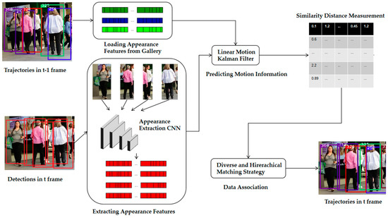
Figure 1.
Proposed multi-object tracking pipeline is illustrated. At the beginning, we load the appearance features of trajectories in the t–1 frame from gallery, and extract the appearance features of detections in the t frame. Then, we predict motion information of the above trajectories and detections by using a Kalman filter. We measure their similarity distance through our proposed equation after obtaining the appearance and motion information. In the end, we match the trajectories and detections with the designed matching strategy.
2.1. Trajectory States
Trajectory states are the basis of our framework. When tracking begins, the tracker receives object detections from the detector. It needs to make a corresponding decision for each detection, such as initialization, tracking, or abandon. The aim is to make the objects have different strategies to solve these problems in different situations, such as occlusion, disappearing, and so on, so as to reduce the number of IDS and Frag.
There are four trajectory states designed in our paper: Tentative, Confirmed, Vanished, and Deleted. The Tentative state is the preparatory stage before an object is formally tracked. All the object detections will stay in this state for several frames, and only those which continuously appear will be considered as true positives (TP). Thus this state can be used to reduce false positives (FP). The Confirmed state is the state in which an object is being correctly tracked, and only in this state can the bounding box of the object be displayed. The Vanished state is the state in which an object disappears or is lost, due to occlusion or drastic changes in appearance. Here, the trajectory will be hidden temporarily so we can reduce the number of IDS and Frag. The Deleted state is the termination state of a trajectory. When it determined that an object no longer appears in the video, it is included in this state.
In order to screen out the error detections, we set the threshold , which represents the required continuous successful matching frames to transfer from Tentative to Confirmed. Additionally, for the purpose of reducing IDS and Frag, we set the threshold , which represents the required continuous unsuccessful matching frames to transfer from Vanished to Deleted.
Figure 2 is an example of the object state transition. At the beginning, the bounding box for the person on the far right side of frame (a) is not displayed, because he just appeared, so his state was Tentative. In frame (b) his state transferred to Confirmed because the object continuously appeared for frames. In frame (c), his state turned to Vanished as a result of being occluded by the purple object. In frame (d), the blue object recovered from the occlusion and his state turned to Confirmed again. At last, in frame (e), he went out of the screen so his state first transferred to Vanished for frames, and then transferred to Deleted until the last.
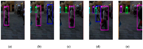
Figure 2.
An example of an object state transition. (a–e) are from MOT17-02-SDP in the MOT17 benchmark dataset. Bounding boxes of different colors represent different objects.
2.2. Trajectory Confidence
Trajectory confidence is an important basis to distinguish whether a trajectory is reasonable or not and whether it can continue to match the new detection. The higher the trajectory confidence, the more likely it is to be the correct trajectory, and vice versa. Generally, there are many factors that determine the trajectory confidence, such as its total length, its length in the Vanished state, the confidence of its historical relevant detections, and its historical similarity distance. Based on the above factors, we define the trajectory confidence as follows:
represents the i-th trajectory in the whole trajectory set,, where represents the number of initial frame of the trajectory and represents the number of terminal frame. represents the trajectory state in frame t. represents the similarity distance between the trajectory and its corresponding historical relevant detections. represents the Intersection over Union (IoU) score between the trajectory and its corresponding historical relevant detections. represents the weighted confidence of the detection which has been associated with the trajectory. Each score is derived from the following equation:
where represents the number of frames that the trajectory successfully matches to the detection, and . indicates that if successfully matches with detection in current frame, it equals to 1, otherwise 0. represents the j-th detection in frame t. represents the similarity distance between and in frame t, which is described in Section 2.4. represents the IoU score between and in frames t. represents the confidence of the j-th detection in frame t, which is given by the detector in advance.
Figure 3 is part of the qualitative tracking results of our algorithm on the MOT15 benchmark dataset. Generally speaking, low confidence trajectories are often caused by overlapping occlusion, dynamic ambiguity, drastic changes in appearance, and other factors. These trajectories are prone to track segmentation, IDS, and other phenomena in subsequent frames. Therefore, we prefer to associate high confidence trajectories with detection targets first, and then deal with low confidence trajectories. The experimental results in Section 3 prove the feasibility of our algorithm.
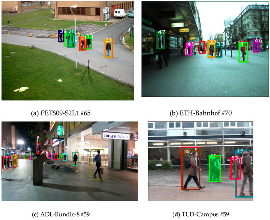
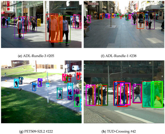
Figure 3.
Exemplary qualitative tracking results for the MOT15 benchmark dataset. (a–d) are from a set of training images and (–h) are from a set of testing images. Following # is the individual frame number in each image sequence. Different trajectories are illustrated in different colors, with different identities marked in white. The red boxes without identities are detections, some of which have not been associated with trajectory. The filled boxes are low-confidence trajectories, while the unfilled rectangles are high-confidence trajectories.
In order to cooperate on our matching strategy, we set the trajectory confidence threshold and the detection confidence threshold according to practical experience, which will be discussed in Section 3.4. Trajectories and detections that exceed the threshold will be classified as high confidence sets, while those below the threshold will be classified as low confidence sets.
2.3. Appearance Feature Extracting Network
A robust appearance feature can prevent the object from drifting to false detection, and can also distinguish the correct object from occlusion. As time goes, the appearance of the object may change gradually, especially for the occluded object. Traditional artificial feature extraction methods imitate the characteristics of human vision and extract features with specific physical meanings. These methods often divide the image into several regions and construct feature vectors or histograms according to the information of multiple local regions. However, they are not perfectly suitable for occlusion and other situations because the artificial feature extraction is not very comprehensive and relatively simple, which often makes it impossible for the tracking algorithm to accurately correlate the same objects of different frames. Therefore, we propose a convolutional neural network based on pedestrian re-identification [17,18].
Following the idea of combining traditional methods with the technology of deep learning, we segment the input image, and then pass all the slices as input into the convolutional neural network. As Figure 4 shows, the original image size was 128 × 64, which is the Global part. In addition, we extend the original image to two other copies, Local Cross and Local Horizontal. Local Cross divides the original image into four local regions with a size of 64 × 32, while Local Horizontal divides the original image into four local regions with a size of 32 × 64. The reasons for our design are as follows.
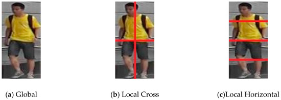
Figure 4.
Region segmentation. The size of the Global part is 128 × 64. The size of the sub-blocks of Local Cross and Local Horizontal are 64 × 32 and 32 × 64, respectively.
Firstly, we design the Local Horizontal patch by referring to the longitudinal distribution of human body structure, like head, trunk, legs, and feet, so that the discriminant ability of our model for pedestrians is reasonably enhanced. Secondly, according to the shooting angle of the camera in the scene, pedestrians are often obscured by one or more parts, therefore they cannot be displayed completely in the image while Local Cross can help the model to enhance its recognition ability on the basis of the different local characteristics of pedestrians. Thirdly, when the global slice and the local slice pass through the convolution neural network, we concatenate their output vectors, which can combine the common area of interest of both the global and local information, further consolidating the model. By artificially designing different feature extraction regions and using neural networks to extract effective features relatively accurately, we can make better use of the advantages of traditional methods and deep learning methods. We will discuss our network structure and experiments in Section 3.3.
2.4. Similarity Distance Measurement
Similarity distance is a metric to measure whether the trajectory and the detection belong to the same object. The smaller the metric is, the more likely they are the same, and vice versa. In this paper, we establish the similarity distance measurement equation from two aspects.
On one hand, in terms of appearance features, although we can get discriminative pedestrian appearance features through our proposed network, it is still difficult for us to correlate and match two identical objects in different frames which are far apart from each other. Therefore, we set up a feature buffer space for each trajectory to store the appearance features of the detections that it has been associated with. When measuring the similarity distance between a trajectory and detection, our method loads all of the trajectory appearance features from its buffer, and calculates the distance between each feature and the detection features. Then, it uses the minimum of the above distance as the similarity distance. In this paper, the appearance features extracted by our CNN has been already normalized, that is, their L2 norm is equal to 1. Then we use the square of Euclidean distance as the similarity distance measurement of appearance features, and define the following equation:
where represents the appearance feature of i-th trajectory and represents the appearance feature of j-th detection. represents the features buffer of i-th trajectory.
In terms of motion characteristics, we introduce the Kalman filter prediction method to assist our algorithm since it is suitable for linear systems, in which the object states obey Gaussian distribution. Meanwhile, many pedestrians move in a linear mode in real scenes, enabling the Kalman filter to predict the uncertain object state more easily. Specifically, we define the measurement space of a trajectory state or a detection as , respectively representing the horizontal and vertical coordinates, width and height, as well as the corresponding velocities of the center point of the trajectory bounding box. In our paper, we use the square of Mahalanobis distance as the measurement standard of motion feature similarity distance, and define the following equation:
where and represent the projection of i-th trajectory state in the measurement space and the covariance matrix of i-th trajectory state in frame t, respectively. represents the measurement space of j-th detection in frame t. In the initial measurement space of a detection, the first four element values are obtained from the prior detector, while the last four element values are initialized to zero. When a track is not associated with any detection, we use the constant velocity linear motion model of the Kalman filter to predict the measurement space of the track directly without correction. Otherwise, when a track is associated with any detection, we update the measurement space of the track according to the detection. Note that when the track state changes from Confirmed to other states, due to occlusion or other reasons, the uncertainty of the track during this period is increased according to the characteristic of the Kalman filter, which may result in a smaller distance between the track and detections, thus we introduce the threshold function as follows. By synthesizing Equations (3) and (4), we define the final similarity distance measurement equation:
where is a threshold function; when is smaller than the threshold, the result of the function is equal to 1, otherwise it is 0. As mentioned above, one of the reasons why we use the threshold function for motion features is that we do not correlate trajectories with detection based on the specific results of the Kalman filter prediction, but only use this to help us screen out some pairs that do not conform to linear motion in terms of motion information, and then use the appearance features to determine how to match the remaining trajectories and detection. Lastly, we need to set a threshold to filter some pairs with too large of a similarity distance of appearance features to reduce the number of FP.
2.5. Diverse and Hierarchical Matching Strategy
The Hungarian algorithm [19] is simple and fast, and is often used in the correlation matching between trajectory and detection. However, it often matches trajectories and detections only according to the loss matrix between them, elements of which are the similarity distance, without considering the need for specific similarity in specific scenarios. For example, at a certain time, two different trajectories have the same similarity with the same detection. According to the Hungarian algorithm, since it is based on global information for correlation matching, it may assign a trajectory to a detection which should not be its match. In this case, we can use other additional information to help us infer how to match the trajectory and detection correctly. The trajectory confidence introduced above is one of the important ways.
Before starting matching, we first divide the current existing trajectories according to the confidence, so that the high confidence trajectories are correlated before the confidence trajectories. We also have to divide the detections into two sets, because the above situation can be reversed, that is, two detections can compete for one trajectory. In addition, instead of dividing all existing trajectories, we must divide the trajectories in the Confirmed and Tentative states. As mentioned in Section 2.1, Vanished and Deleted states are equivalent to two situations in which the object disappears, so we don’t need to consider their confidence. To sum up, we design Algorithm 1 for data association.
First of all, we take the trajectory set and detections set of the current frame as input. In line 1, we divide the trajectories in different states and we calculate the confidence of trajectories in Confirmed and Tentative states according to Equations (1) and (2), and divide the trajectory sets with high and low confidence according to the confidence threshold mentioned in Section 2.2. Similarly, we divide the detection set into high and low confidence sets. In line 3, we calculate the similarity matrix between the current trajectory and the detection according to Equations (3), (4), and (5).
After the preparations have been completed, in line 4 we use the Hungarian algorithm to match the high and low confidence trajectory sets and the detection set in order of their priority, to ensure that the correct matches are matched in advance, so as to reduce the number of FP. Since the drastic change of appearance caused by occlusion, illumination, or other reasons may affect the appearance characteristics of the object and make the similarity measurement inaccurate when the moving distance of the object between two continuous frames is not large, in line 5 we make IoU matching for the remaining unmatched Confirmed and Tentative trajectory sets and the detection set. In line 6, we match the trajectories in the Vanished state only according to the appearance similarity matrix. The reason for this is that the current position of trajectories in the Vanished state may be far from their positions before they disappear, and it is unreasonable to predict them in motion information. Therefore, we do not use the total similarity equation correlate here.
Finally, we update the matching pairs, unmatched trajectory sets, and unmatched detection sets in lines 7–9 and return them in line 10; thus we then can update and initialize the trajectories.
| Algorithm 1. Trajectories Association |
| Input: Trajectories set K, Detections set D |
| Output: Set of unmatched trajectories , set of unmatched detections , set of matches |
| 1: Initialize set of confirmed and tentative trajectories and set of vanished trajectories , set of high-confidence trajectories and set of low-confidence trajectories , set of high-confidence detections and set of low-confidence detections |
| 2: Initialize , and to |
| 3: Compute affinity matrix and appearance affinity matrix using Equation: (3) (4) (5) |
| 4: Associate and , and , and , and according to |
| 5: Associate remaining trajectories and remaining and according to IoU |
| 6: Associate and remaining and according to |
| 7: Update to remaining trajectories |
| 8: Update to remaining detections |
| 9: Update to successful matches |
| 10: return , , |
3. Experiments
3.1. Dataset
We evaluated the proposed online multi-object tracking algorithm on the MOT15 benchmark dataset and MOT17 benchmark dataset. The MOT15 benchmark dataset includes 11 training videos and 11 test videos. The MOT17 benchmark dataset is among the latest online challenges in tracking, which contains seven training videos and seven test videos, with three different detectors of objects, namely SDP (Session Description Protocol) [20], Faster-RCNN(Region convolution neural network) [21] and DPM( Direct Part Marking) [22] respectively. The resolution, length, and number of each video are different, and the videos include static and dynamic cameras, dense and sparse crowds, indoor and outdoor scenes of public places, and other scenarios. The annotations are basically correct. In summary, these are comprehensive datasets for evaluating multi-object tracking algorithm.
In addition, we evaluated our deep appearance feature extracting network on a public pedestrian re-identification dataset, Market1501 [23]. The dataset contains more than 32,000 images of pedestrians, including 1501 different identities; each person is composed of two to six cameras.
3.2. Evaluation Metrics
We used the evaluation metrics [13,24,25] of the MOT benchmark dataset as our measurement metrics. The higher the score, the better the metric with (↑) and the worse the metric with (↓). These metrics include:
MOTA(↑)[24]: Multiple Object Tracking Accuracy, combines three error sources: false positives, missed objects, and identity switches.
MT(↑): Mostly tracked objects. The ratio of ground-truth trajectories that are covered by a track hypothesis for at least 80% of their respective life spans.
ML(↓): Mostly lost objects. The ratio of ground-truth trajectories that are covered by a track hypothesis for at most 20% of their respective life spans.
FP(↓): The total number of false positives.
FN(↓): The total number of false negatives.
IDS(↓): The total number of identity switches.
Frag(↓): The total number of times a trajectory is fragmented.
FPS(↑): The processing speed in frames per second on the benchmark excluding the detector.
3.3. Implementation Details
In order to extract the appearance features in real time, we needed to train our network on the pedestrian re-identification dataset in advance. In this paper, we trained it on a public dataset, Market1501 [23]. Our network structure is shown in Table 1. In terms of width, we divided it into three parts as mentioned in Section 2.3. In terms of depth, we had a total of seven convolution blocks for the global part, and only four convolution blocks for the local part. These convolution blocks mainly refer to residual blocks in the wide residual network (ResNet) [26], which has the characteristics of smaller parameters and more efficient performance. In order to solve the vanishing gradient problem and ensure that the accuracy of the deep layer network is not lower than the shallow layer network, ResNet introduced a skip connection. By directly adding the output of the upper layer to lower layer, the output of the two layers could be identically mapped, which means it maintains the optimal accuracy of the network without any modification to the optimal features. After convoluting each region by different blocks, we got the relatively deep semantic information of the global region and the shallow semantic information of the two local regions. Then, we attached a full connection layer and a batch and L2 normalization layer to the network. By combining the 128-dimensional global feature with two 256-dimensional local features, we got a 640-dimensional appearance feature from the last layer.

Table 1.
Proposed appearance extracting structure. MP: Max-Pooling; S: Stride; SL: Slice; CA: Concatenation; G: Global; LC: Local Cross; LH: Local Horizontal.
Our appearance feature extraction was implemented in Tensorflow [27] and tested on a PC with Intel core i7-7700 CPU, 16 GB RAM, and Nvidia GTX 1070 GPU, while our tracking part was implemented in Python and tested on the same PC. In the training, we used cosine softmax loss [28] as our loss function and Adam [29] as the optimizer with a learning rate of 1xe-3. It took about 50,000 iterations to converge the model. We evaluated our model on the Market1501 test set and achieved a result of mAP = 0.595. In comparison, the AlexNet identification model reached a result of mAP = 32.36 while the ResNet-50 identification model reached a result of mAP = 47.78 in [30], proving that our model had certain discrimination for pedestrians. When it was actually applied to multi-target tracking, we extracted the appearance features of more than 460 detections in a second on the PC. In fact, there was only about 10 to 20 detections in one frame. Therefore, our appearance feature extracting network can fully meet the requirements of real-time tracking.
It takes about 32 seconds and 130 seconds to generate the output results of the MOT15 test set and the MOT17 test set on the same PC, while it takes approximately 122 seconds and 371 seconds to extract the appearance features of all the detections in the two test sets using the network we designed. The reason why the MOT17 test set takes much longer than the MOT15 test set is that the number of detections in the MOT17 test set (including DPM, FRCNN, and SDP) is much larger than that in the MOT15 test set, and the additional calculation time was mainly spent on extracting the appearance features.
3.4. Ablation Studies
In order to prove the validity of each part of our algorithm, we disabled the functions of each part of the algorithm and evaluated them on the MOT15 training set. As shown in Table 2, the Proposed Algorithm is the result of the complete algorithm in our paper.
Table 2.
Performance of our method when different components are disabled.
As can be seen from the Table 2, each part of the algorithm has a certain impact on the whole algorithm. Among them, deep appearance features have the largest impact on MOTA, MT, and ML. The results support that DAFs are much more discriminative than traditional features. Trajectory states and state transitions also have a great influence. This method helps us greatly reduce the number of IDS, FP, and Frag, but at the same time it also adds a lot of FN. This is because the trajectory is not shown in the Tentative state, which causes the tracker to miss many supposedly correct trajectories, but also as a result of this the tracker can screen out many false detections. In fact, our matching strategy also depends on the designed trajectory states, which are also affected to some extent. Additionally, similarity distance measurements and diverse and hierarchical matching strategies also have certain impact on the metrics to different degrees.
In order to study the impact of numerous thresholds or weights on the algorithm, we have done a lot of comparative experiments. Since there are too many parameters involved, this paper does not list them one by one. Here, we take the threshold mentioned in Section 2.1 as an example, as shown in Table 3. From the table, we can see that the number of MT, FP, IDS, and Frag gradually decreased while ML and FN gradually increased with the increase of threshold. This also proves that our algorithm misses the correct trajectory while eliminating the error detection. The number of MOTA first increased and then decreased, reaching its maximum at 2, so we let in the following experiments. Similarly, we got the best value of other threshold parameters on the MOT15 benchmark dataset through experimental data, including , , , , , , where the value were obtained from the table of critical values of chi-square distribution.
Table 3.
Performance of our method under different .
3.5. Evaluations on MOT15
To verify the efficiency of our method, as shown in Table 4, we exhibit part of the experimental results, where our method is denoted by HMB_DAF (Hierarchical-Matching-Based MOT with Deep Appearance Features). All the results in Table 4 were generated using public detection sets of the MOT15 benchmark as an input. In order to make a fair and effective comparison, we gathered some online methods published in recent years as the baseline methods, which also attach great importance to data association and make full use of appearance features. However, since many works did not publish the FPS of their methods as well as non-open sources, we only choose those methods which can be accessed publicly for fair comparison.
Table 4.
Tracking performance on the MOT15 dataset. Best results in each category appear in bold. (A) Traditional method, (B) deep learning method. Our method is denoted by HMB_DAF.
As can be seen in Table 4, although our method cannot outperform AMIR15 or MDP in terms of MOTA, we surpassed most algorithms in speed. Moreover, our FP was the lowest, which proves the effectiveness of our algorithm in handling error detection. However, as mentioned in Section 3.4, our FN was relatively high, leading to the low MT rate, but overall it had little effect on the comprehensive metric. Compared with the traditional MOT methods, our MOTA was higher except for MDP, which utilized machine learning to reinforcement its data association part, leading to low FPS. Compared with deep learning methods, our advantage mainly lies in FPS, as a result of their multiple complex network structures in each part of methods. For example, AMIR15 [9] designed three RNNs for object appearance, motion, and interaction separately in order to calculate the similarity between detections and objects. In contrast, we only used deep learning in feature extraction, which was a trade-off between accuracy and speed. By exploiting the bounding box regression of an object detector, Tracktor++ [38] converted the detector into a tracktor, such as Faster-RCNN, which could predict the position of an object in the next frame after training the network on the MOT17Det [15]. In contrast, we only considered the public detections as the input of our tracktor, instead of directly generating other detections or applying object detection techniques in MOT, which would significantly increase consumption times and training costs.
3.6. Evaluations on MOT17
Similarly to the experiment on the MOT15 dataset, we used the public detection results of the MOT17 benchmark dataset as the input detections of the algorithm, and compared it with other excellent methods. For a fair comparison, these baseline methods are all online and they are also dependent on the appearance cue. Parts of the experimental results are shown in Table 5. Identically, we only choose those accessible published methods for fair comparison.
Table 5.
Tracking performance on the MOT17 dataset. Best results in each category appear in bold. (A) Traditional method, (B) deep learning method. Our method is denoted by HMB_DAF.
Compared to the MOT15 dataset, the detections provided in the MOT17 dataset were much precise, leading to our relatively higher MT score and lower FN score. It proved that our method relies heavily on detections as well. The more accurate the detection, the better the performance of our method. It is worth mentioning that GMPHD_DAL [12] also utilized pedestrian re-identification technology. The difference is that we trained our appearance extraction network on a pedestrian re-ID dataset while GMPHD_DAL was applied on the data association part for object re-matching. Although our MOTA was only 1% higher than GMPHD_DAL, there was still an obvious gap in IDS, Frag, and FPS, which further highlights the effectiveness of our method.
4. Conclusions
In this paper, we proposed a hierarchical matching based online and real-time multi-object tracking approach with deep appearance features. A hierarchical data association strategy can effectively reduce the number of FP, IDS, and other metrics while maintaining high real-time accuracy. In order to cooperate with the data association strategy, we designed our model in four aspects: Firstly, we have designed different trajectory states and state transitions, which can reasonably manage trajectory allocation and deal with missing objects and false object; secondly, we have defined trajectory confidence based on position information, appearance information, and history-related detection information of trajectory, so as to help us to diversify strong and weak trajectories; thirdly, we have combined traditional methods with deep learning methods and designed a deep convolution neural network, which has been trained on a large-scale pedestrian re-identification dataset to help us extract discriminant pedestrian appearance features; fourthly, we have designed a similarity distance measurement based on appearance features and motion features, so that we can get the proximate similarity score between the trajectory and the detection.
We have studied the influence of each part of the algorithm in a comparative experiment and achieved excellent results on the MOT15 and MOT17 benchmark datasets, showing the effectiveness of our algorithm. In future work, we will do more experimental research on our approach and improve a series of shortcomings in this paper, such as studying the relationship among the various parameters, reducing the number of FN, and raising the number of MT.
Author Contributions
Q.J. conceived and designed the experiments; H.Y. and X.W. performed the experiments and wrote the paper. All authors have read and agreed to the published version of the manuscript.
Funding
This research received no external funding.
Acknowledgments
This research was supported by the Key R&D Program of Guangdong Province (2018B010107005) and the Natural Science Foundation of Guangdong Province, China (No.2016A030313288). We would like to thank the anonymous reviewers for their suggestions and comments.
Conflicts of Interest
The authors declare no conflict of interest.
References
- Wang, X. Intelligent multi-camera video surveillance: A review. Pattern Recognit. Lett. 2013, 34, 3–19. [Google Scholar] [CrossRef]
- Candamo, J.; Shreve, M.; Goldgof, D.B.; Sapper, D.B.; Kasturi, R. Understanding transit scenes: A survey on human behavior-recognition algorithms. IEEE Trans. Intell. Transp. Syst. 2010, 11, 206–224. [Google Scholar] [CrossRef]
- Uchiyama, H.; Marchand, E. Object Detection and Pose Tracking for Augmented Reality: Recent Approaches. Available online: https://hal.inria.fr/hal-00751704/document (accessed on 29 March 2020).
- Meijering, E.; Dzyubachyk, O.; Smal, I.; van Cappellen, W.A. Tracking in cell and developmental biology. Semin. Cell Dev. Biol. 2009, 20, 894–902. [Google Scholar] [CrossRef] [PubMed]
- Girshick, R.; Donahue, J.; Darrell, T.; Jitendra, M.; Berkeley, U.C.; ICSI. Rich feature hierarchies for accurate object detection and semantic segmentation. In Proceedings of the IEEE Conference on Computer Vision and Pattern Recognition, Washington, DC, USA, 24–27 June 2014; pp. 580–587. [Google Scholar] [CrossRef]
- Redmon, J.; Divvala, S.; Girshick, R.; Ali, F. You only look once: Unified, real-time object detection. In Proceedings of the IEEE conference on computer vision and pattern recognition, Las Vegas, NV, USA, 27–30 June 2016; pp. 779–788. [Google Scholar] [CrossRef]
- Liu, W.; Anguelov, D.; Erhan, D.; Christian, S.; Scott, R.; Fu, C.-Y.; Alexander, C.B. SSD: Single Shot MultiBox Detector. In European Conference on Computer Vision; Springer: Amsterdam, The Netherlands, 2016. [Google Scholar] [CrossRef]
- Dalal, N.; Triggs, B. Histograms of Oriented Gradients for Human Detection. In Proceedings of the Computer Vision and Pattern Recognition, San Diego, CA, USA, 20–26 June 2005; pp. 886–893. [Google Scholar] [CrossRef]
- Sadeghian, A.; Alahi, A.; Savarese, S. Tracking The Untrackable: Learning To Track Multiple Cues with Long-Term Dependencies. In Proceedings of the ICCV, Venice, Italy, 22–29 October; 2017. [Google Scholar]
- Wu, H.; Hu, Y.; Wang, K.; Li, H.; Nie, L.; Cheng, H. Instance-Aware Representation Learning and Association for Online Multi-Person Tracking. Pattern Recognit. 2019, 94, 25–34. [Google Scholar] [CrossRef]
- Yoon, K.; Gwak, J.; Song, Y.M.; Yoon, Y.C.; Jeon, M.G. OneShotDA: Online Multi-Object Tracker with One-Shot-Learning-Based Data Association. IEEE Access 2020, 8, 38060–38072. [Google Scholar] [CrossRef]
- Baisa, N.L. Online multi-object visual tracking using a GM-PHD filter with deep appearance learning. In Proceedings of the 2019 22nd International Conference on Information Fusion (FUSION), Shaw Center, OT, Canada, 2–5 July 2019. [Google Scholar]
- Ristani, E.; Solera, F.; Zou, R.; Rita, C.; Carlo, T. Performance measures and a data set for multi-target, multi-camera tracking. In Proceedings of the European Conference on Computer Vision Springer, Amsterdam, The Netherlands, 8–16 October 2016; pp. 17–35. [Google Scholar] [CrossRef]
- Leal-Taixé, L.; Milan, A.; Reid, I.; Roth, S.; Schindler, K. MOTChallenge 2015: Towards a Benchmark for Multi-object Tracking. ArXiv 2015, arXiv:1504.01942. Available online: https://arxiv.org/abs/1504.01942 (accessed on 29 March 2020).
- Milan, A.; Leal-Taixé, L.; Reid, I.; Roth, S.; Schindler, K. MOT16: A Benchmark for Multi-Object Tracking. ArXiv 2016, arXiv:1603.00831. Available online: https://arxiv.org/pdf/1603.00831.pdf (accessed on 29 March 2020).
- Kalman, R. A New Approach to Linear Filtering and Prediction Problems. J. Basic Eng. 1960, 82, 35–45. [Google Scholar] [CrossRef]
- Varior, R.R.; Shuai, B.; Lu, J.; Xu, D.; Wang, G. A Siamese Long Short-Term Memory Architecture for Human Re-Identification. In European Conference on Computer Vision; Springer: Amsterdam, The Netherlands, 2016. [Google Scholar]
- He, L.; Liang, J.; Li, H.; Sun, Z. Deep Spatial Feature Reconstruction for Partial Person Re-Identification: Alignment-Free Approach. In Proceedings of the 2018 IEEE/CVF Conference on Computer Vision and Pattern Recognition, Salt Lake City, UT, USA, 18–23 June 2018; 2018. [Google Scholar] [CrossRef]
- Kuhn, H.W. The hungarian method for the assignment problem. Nav. Res. Logist. Q. 1995, 2, 83–97. [Google Scholar] [CrossRef]
- Yang, F.; Choi, W.; Lin, Y. Exploit All the Layers: Fast and Accurate CNN Object Detector with Scale Dependent Pooling and Cascaded Rejection Classifiers. In Proceedings of the 2016 IEEE Conference on Computer Vision and Pattern Recognition (CVPR), Las Vegas, NV, USA, 27–30 June 2016; pp. 2129–2137. [Google Scholar] [CrossRef]
- Ren, S.; He, K.; Girshick, R.; Sun, J. Faster R-CNN: Towards Real-Time Object Detection with Region Proposal Networks. IEEE Trans. Pattern Anal. Mach. Intell. 2017, 39, 1137–1149. [Google Scholar] [CrossRef] [PubMed]
- Felzenszwalb, P.F.; Girshick, R.B.; McAllester, D.; Ramanan, D. Object detection with discriminatively trained partbased models. IEEE Trans. Pattern Anal. Mach. Intell. 2010, 32, 1627–1645. [Google Scholar] [CrossRef] [PubMed]
- Zheng, L.; Shen, L.; Tian, L.; Wang, S.; Wang, J.; Tian, Q. Scalable Person Re-identification: A Benchmark. In Proceedings of the IEEE International Conference on Computer Vision (ICCV), Santiago, Chile, 7–13 December 2015; pp. 1116–1124. [Google Scholar] [CrossRef]
- Bernardin, K.; Stiefelhagen, R. Evaluating Multiple Object Tracking Performance: The CLEAR MOT Metrics. Image Video Process. 2008, 1, 1–10. [Google Scholar] [CrossRef]
- Li, Y.; Huang, C.; Nevatia, R. Learning to associate: Hybrid Boosted multi-object tracker for crowded scene. In Proceedings of the IEEE Computer Society Conference on Computer Vision and Pattern Recognition, Miami, FL, USA, 20–26 June 2009. [Google Scholar] [CrossRef]
- Zagoruyko, S.; Komodakis, N. Wide residual networks. In Proceedings of the BMVC, York, UK, 19–22 September 2016; pp. 1–12. [Google Scholar] [CrossRef]
- Abadi, M.; Agarwal, A.; Barham, P.; Brevdo, E.; Chen, Z.; Citro, C.; Corrado, G.S.; Davis, A.; Dean, J.; Devin, M.; et al. TensorFlow: Large-Scale Machine Learning on Heterogeneous Distributed Systems. Arxiv 2016, arXiv:1603.04467v2. Available online: https://arxiv.org/abs/1603.04467 (accessed on 29 March 2020).
- Wojke, N.; Bewley, A. Deep Cosine Metric Learning for Person Re-identification. In Proceedings of the 2018 IEEE Winter Conference on Applications of Computer Vision (WACV), Lake Tahoe, NV, USA, 12–15 March 2018; pp. 748–756. [Google Scholar] [CrossRef]
- Kingma, D.P.; Ba, J. Adam: A method for stochastic optimization. In Proceedings of the International Conference on Learning Representations, San Diego, CA, USA, 7–9 May 2015. [Google Scholar]
- Zheng, L.; Yang, Y.; Hauptmann, A.G. Person Re-identification: Past, Present and Future. ArXiv 2016, arXiv:1610.02984, Available online: https://arxiv.org/abs/1610.02984 (accessed on 29 March 2020).
- Dalal, N.; Triggs, B. Histograms of oriented gradients for human detection[C]. International Conference on computer vision & Pattern Recognition (CVPR’05). IEEE Comput. Soc. 2005, 1, 886–893. [Google Scholar]
- Song, Y.; Jeon, M. Online multiple object tracking with the hierarchically adopted gm-phd filter using motion and appearance. In Proceedings of the Consumer Electronics-Asia (ICCE-Asia), Seoul, Korea, 26–28 October 2016; pp. 1–4. [Google Scholar] [CrossRef]
- Ju, J.; Kim, D.; Ku, B.; David, K.H.; Hanseok, K. Online multi-person tracking with two-stage data association and online appearance model learning. Iet Comput. Vis. 2017, 11, 87–95. [Google Scholar] [CrossRef]
- Anh, N.T.L.; Khan, F.M.; Negin, F.; Francois, B. Multi-Object tracking using multi-channel part appearance representation, Advanced Video and Signal Based Surveillance (AVSS). In Proceedings of the 2017 14th IEEE International Conference on San Francisco, San Francisco, CA, USA, 4–8 August 2017; pp. 1–6. [Google Scholar] [CrossRef]
- Sanchez-Matilla, R.; Poiesi, F.; Cavallaro, A. Online multi-target tracking with strong and weak detections. In Proceedings of the European Conference on Computer Vision, Amsterdam, The Netherlands, 8–16 October 2016; pp. 84–99. [Google Scholar] [CrossRef]
- Xiang, Y.; Alahi, A.; Savarese, S. Learning to Track: Online Multi-Object Tracking by Decision Making. In Proceedings of the International Conference on Computer Vision (ICCV), Araucano Park, Chile, 11–18 December 2015. [Google Scholar]
- Chul, Y.; Song, Y.-M.; Yoon, K.; Jeon, M. Online Multi-Object Tracking Using Selective Deep Appearance Matching; IEEE: Jeju, Korea, 2018; pp. 206–212. [Google Scholar] [CrossRef]
- Bergmann, P.; Meinhardt, T.; Leal-Taixe, L. Tracking without bells and whistles. In Proceedings of the IEEE International Conference on Computer Vision, Seoul, Korea, 27–28 October 2019; pp. 941–951. [Google Scholar]
- Eiselein, V.; Arp, D.; Patzold, M.; Sikora, T. Real-Time Multi-human Tracking Using a Probability Hypothesis Density Filter and Multiple Detectors; IEEE Computer Society: NW Washington, DC, USA, 2012. [Google Scholar] [CrossRef]
- Kutschbach, T.; Bochinski, E.; Eiselein, V.; Sikora, T. Sequential Sensor Fusion Combining Probability Hypothesis Density and Kernelized Correlation Filters for Multi-Object Tracking in Video Data; IEEE: Lecce, Italy, 2017. [Google Scholar] [CrossRef]
- Baisa, N.L.; Wallace, A. Development of a N-type GM-PHD filter for multiple target, multiple type visual tracking. J. Vis. Commun. Image Represent. 2019, 59, 257–271. [Google Scholar] [CrossRef]
- Lee, S.; Kim, E. Multiple Object Tracking via Feature Pyramid Siamese Networks. IEEE Access 2019, 7, 8181–8194. [Google Scholar] [CrossRef]


© 2020 by the authors. Licensee MDPI, Basel, Switzerland. This article is an open access article distributed under the terms and conditions of the Creative Commons Attribution (CC BY) license (http://creativecommons.org/licenses/by/4.0/).