Optimizing Convolutional Neural Network Hyperparameters by Enhanced Swarm Intelligence Metaheuristics


Abstract
1. Introduction
1.1. Swarm Intelligence Metaheuristic and Literature Review
1.2. Research Objectives and Paper’s Structure
2. Problem Formulation and Related Literature Review
2.1. Metaheuristics Applications for CNN Optimization
2.2. Mathematical Model
3. Proposed Swarm Intelligence Approaches
3.1. Original Tree Growth Algorithm Overview
- Group of the best trees;
- Group of trees that are competing for light;
- Remove or replace group;
- Reproduction group.
3.2. Enhanced Tree Growth Algorithm
| Algorithm 1 Pseudocode of the exploitation enhanced TGA (EE-TGA). |
|
3.3. Original Firefly Algorithm Overview
- Each firefly is unisex and can be attracted by any other firefly;
- The brightness determines the fireflies’ attractiveness; as the distance become shorter, the attractiveness of fireflies increases, and they become brighter;
- The fireflies’ brightness determines the fitness function.
3.4. Enhanced Firefly Algorithm
| Algorithm 2 Pseudocode of the exploitation and exploration enhanced FA (-FA). |
|
4. CNN Optimization Simulation Environment, the Algorithms’ Adaptations, and Parameter Setup
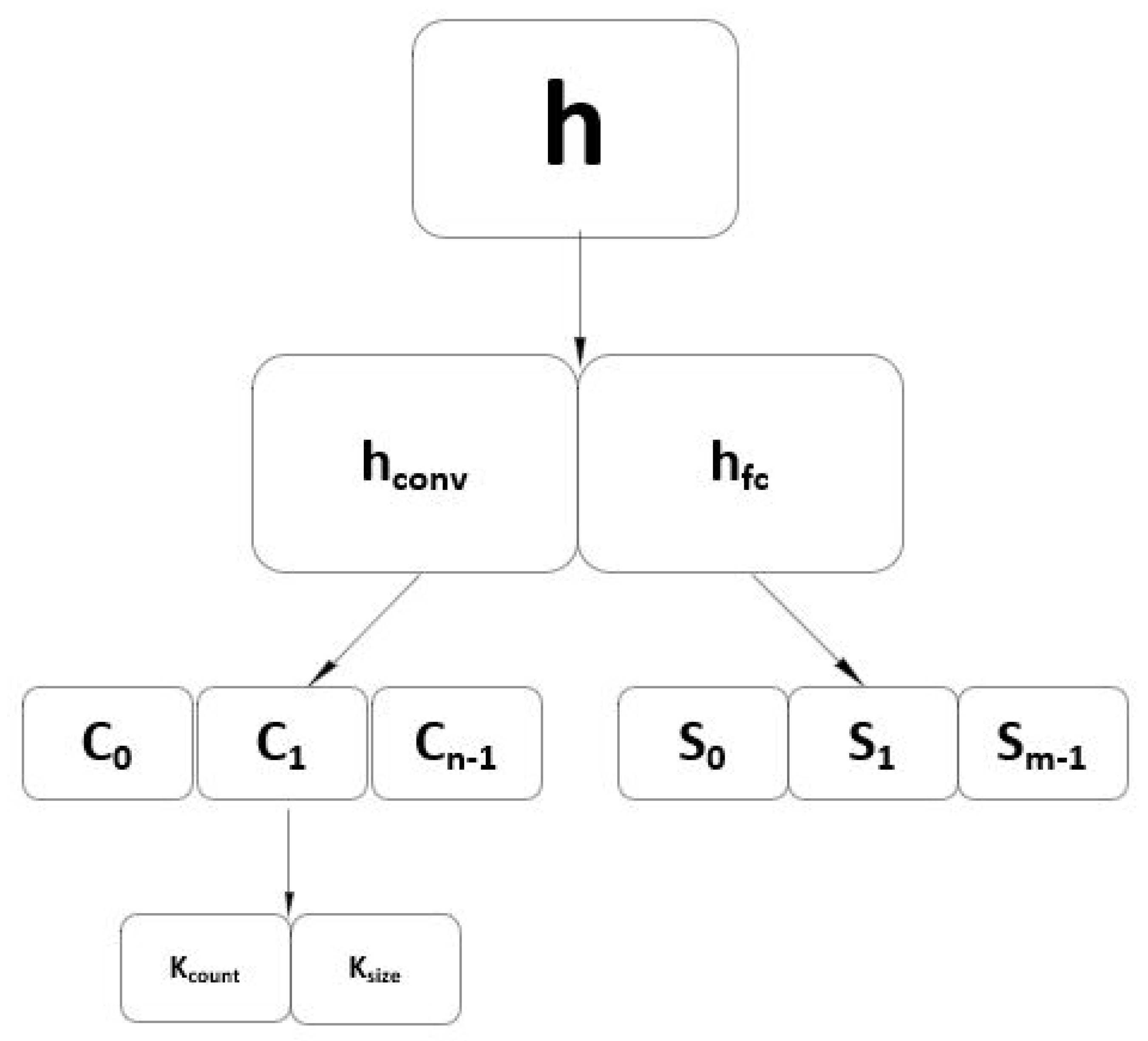
4.1. Solutions’ Encoding and Algorithms’ Adaptations
| Algorithm 3 High-level procedure of the CNN design framework. |
|
4.2. Parameter Setup
5. Experimental Results and Discussion
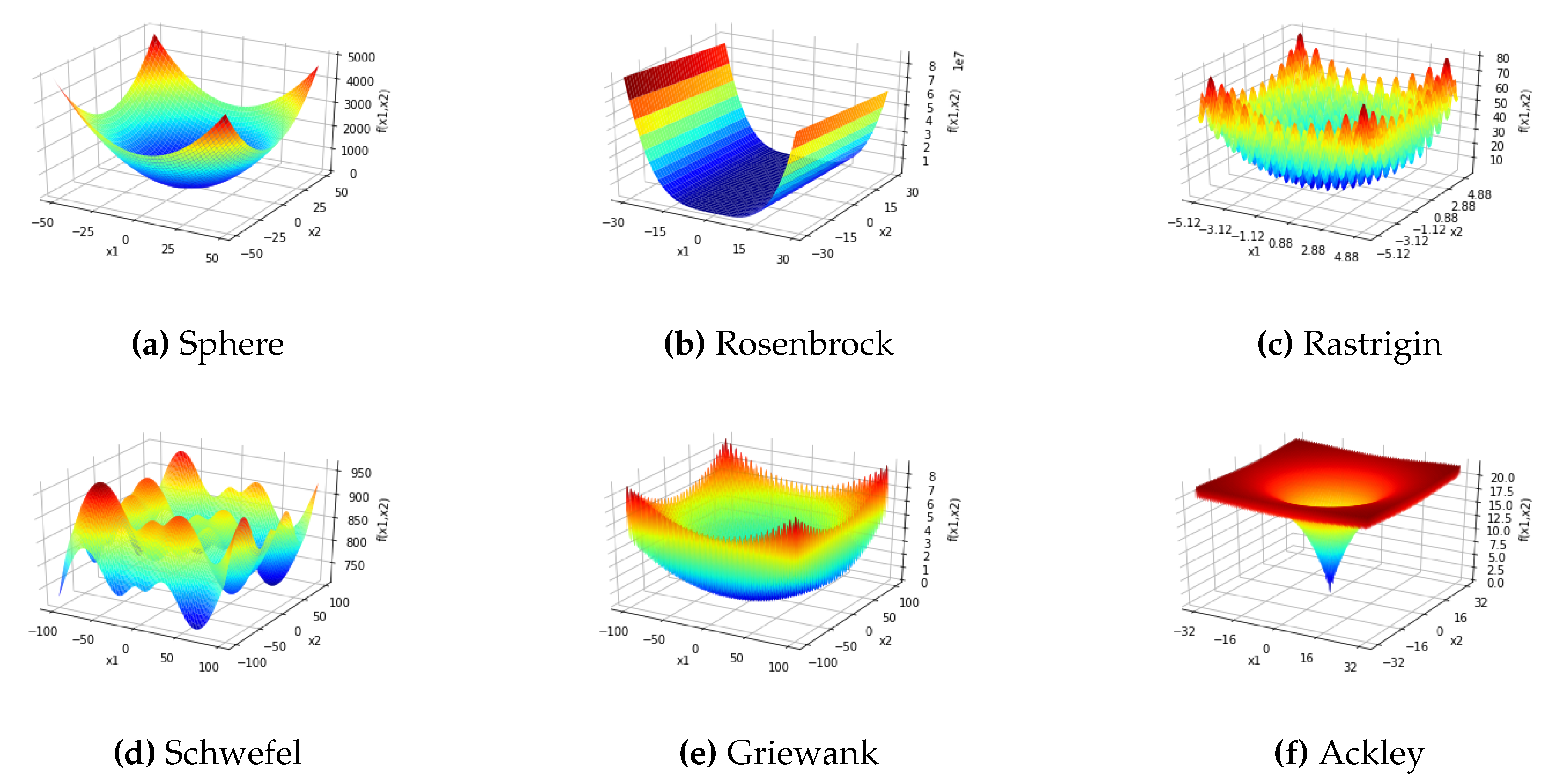
5.1. Performance Evaluation of EE-TGA and -FA on Standard Unconstrained Benchmarks
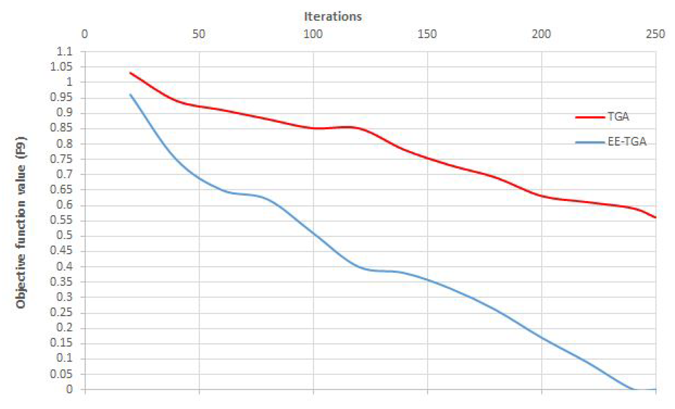
5.1.1. Performance Evaluation of EE-TGA
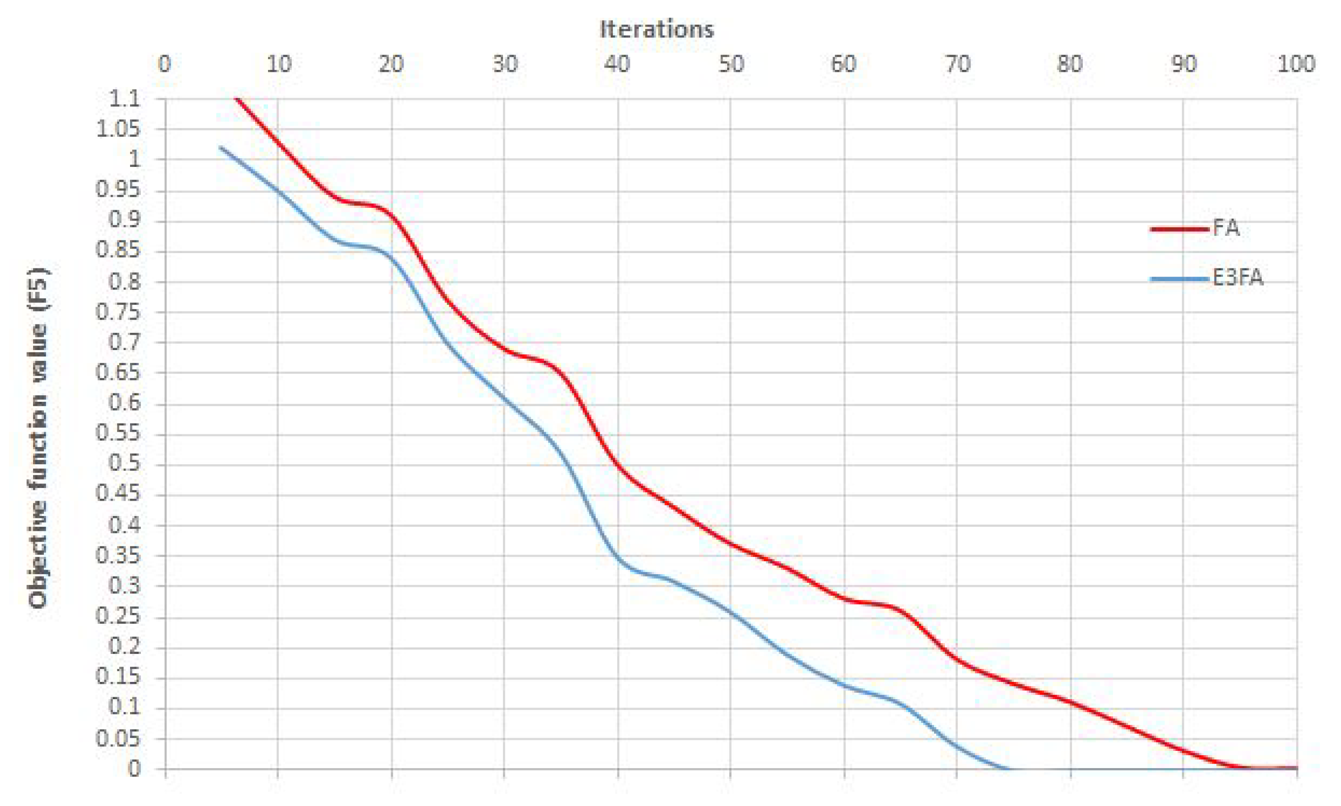
5.1.2. Performance Evaluation of -FA
5.1.3. EE-TGA and FA Benchmark Simulations’ Overall Conclusion
5.2. Convolutional Neural Network Hyperparameter Optimization Experiments
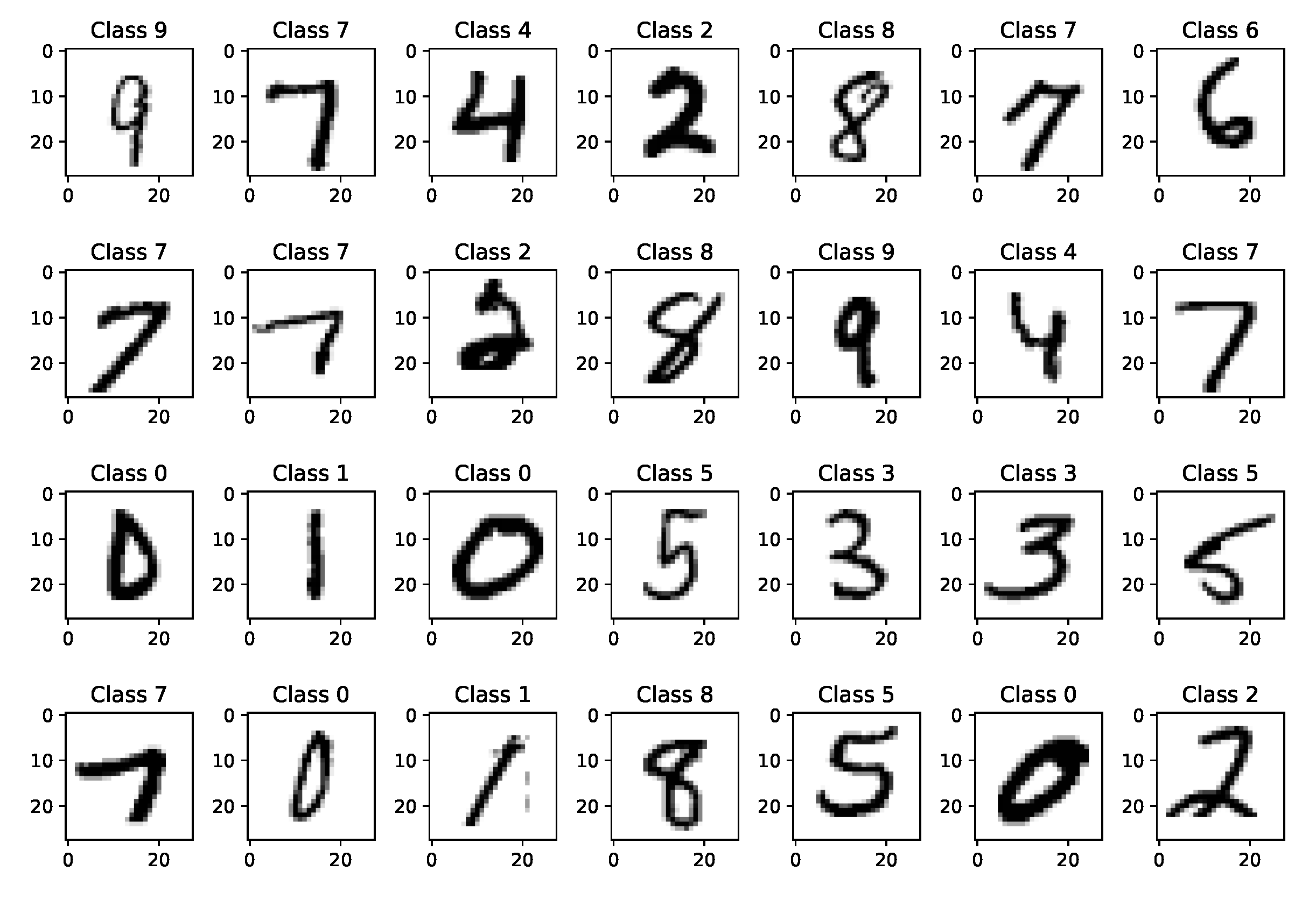
5.2.1. Benchmark Dataset
5.2.2. Convolutional Neural Network Hyperparameter Optimization Results and Analysis
6. Conclusions
Author Contributions
Funding
Conflicts of Interest
References
- Ren, S.; He, K.; Girshick, R.B.; Sun, J. Faster R-CNN: Towards Real-Time Object Detection with Region Proposal Networks. Available online: Advancesinneuralinformationprocessingsystems (accessed on 10 February 2020).
- Farabet, C.; Couprie, C.; Najman, L.; LeCun, Y. Learning Hierarchical Features for Scene Labeling. IEEE Trans. Pattern Anal. Mach. Intell. 2013, 35, 1915–1929. [Google Scholar] [CrossRef] [PubMed]
- Karpathy, A.; Fei-Fei, L. Deep visual-semantic alignments for generating image descriptions. In Proceedings of the IEEE Conference on Computer Vision and Pattern Recognition, Las Vegas, NV, USA, 26 June–1 July 2015; pp. 3128–3137. [Google Scholar]
- Taigman, Y.; Yang, M.; Ranzato, M.; Wolf, L. DeepFace: Closing the Gap to Human-Level Performance in Face Verification. In Proceedings of the 2014 IEEE Conference on Computer Vision and Pattern Recognition, Columbus, OH, USA, 23–28 June 2014; pp. 1701–1708. [Google Scholar]
- Toshev, A.; Szegedy, C. DeepPose: Human Pose Estimation via Deep Neural Networks. In Proceedings of the 2014 IEEE Conference on Computer Vision and Pattern Recognition, Columbus, OH, USA, 23–28 June 2014; pp. 1653–1660. [Google Scholar]
- Lecun, Y.; Bottou, L.; Bengio, Y.; Haffner, P. Gradient-based learning applied to document recognition. Proc. IEEE 1998, 86, 2278–2324. [Google Scholar] [CrossRef]
- Krizhevsky, A.; Sutskever, I.; Hinton, G.E. ImageNet Classification with Deep Convolutional Neural Networks. Available online: http://papers.nips.cc/paper/4824-imagenet-classification-with-deep-convolutional-neural-networks.pdf (accessed on 10 February 2020).
- Simonyan, K.; Zisserman, A. Very Deep Convolutional Networks for Large-Scale Image Recognition. arXiv 2004, arXiv:1409.1556. Available online: https://arxiv.org/pdf/1409.1556.pdf (accessed on 10 February 2020).
- Szegedy, C.; Liu, W.; Jia, Y.; Sermanet, P.; Reed, S.; Anguelov, D.; Erhan, D.; Vanhoucke, V.; Rabinovich, A. Going deeper with convolutions. In Proceedings of the 2015 IEEE Conference on Computer Vision and Pattern Recognition (CVPR), Boston, MA, USA, 7–12 June 2015; pp. 1–9. [Google Scholar]
- He, K.; Zhang, X.; Ren, S.; Sun, J. Deep Residual Learning for Image Recognition. In Proceedings of the 2016 IEEE Conference on Computer Vision and Pattern Recognition (CVPR), Las Vegas, NV, USA, 27–30 June 2016. [Google Scholar]
- Huang, G.; Liu, Z.; v. d. Maaten, L.; Weinberger, K.Q. Densely Connected Convolutional Networks. In Proceedings of the 2017 IEEE Conference on Computer Vision and Pattern Recognition (CVPR), Honolulu, HI, USA, 21–26 July 2017; pp. 2261–2269. [Google Scholar]
- Hu, J.; Shen, L.; Sun, G. Squeeze-and-Excitation Networks. In Proceedings of the 2018 IEEE/CVF Conference on Computer Vision and Pattern Recognition, Salt Lake City, UT, USA, 18–23 June 2018. [Google Scholar]
- Wang, Y.; Zhang, H.; Zhang, G. cPSO-CNN: An efficient PSO-based algorithm for fine-tuning hyper-parameters of convolutional neural networks. Swarm Evol. Comput. 2019, 49, 114–123. [Google Scholar] [CrossRef]
- Darwish, A.; Ezzat, D.; Hassanien, A.E. An optimized model based on convolutional neural networks and orthogonal learning particle swarm optimization algorithm for plant diseases diagnosis. Swarm Evol. Comput. 2020, 52, 100616. [Google Scholar] [CrossRef]
- Suganuma, M.; Shirakawa, S.; Nagao, T. A Genetic Programming Approach to Designing Convolutional Neural Network Architectures. In Proceedings of the Genetic and Evolutionary Computation Conference, New York, NY, USA, 15–19 July 2017; pp. 497–504. [Google Scholar]
- Qolomany, B.; Maabreh, M.; Al-Fuqaha, A.; Gupta, A.; Benhaddou, D. Parameters optimization of deep learning models using Particle swarm optimization. In Proceedings of the 13th International Wireless Communications and Mobile Computing Conference (IWCMC), Valencia, Spain, 26–30 June 2017; pp. 1285–1290. [Google Scholar]
- Bochinski, E.; Senst, T.; Sikora, T. Hyper-parameter optimization for convolutional neural network committees based on evolutionary algorithms. In Proceedings of the 2017 IEEE International Conference on Image Processing (ICIP), Beijing, China, 17–20 September 2017; pp. 3924–3928. [Google Scholar]
- de Rosa, G.H.; Papa, J.P.; Yang, X.S. Handling dropout probability estimation in convolution neural networks using meta-heuristics. Soft Comput. 2018, 22, 6147–6156. [Google Scholar] [CrossRef]
- Yamasaki, T.; Honma, T.; Aizawa, K. Efficient Optimization of Convolutional Neural Networks Using Particle Swarm Optimization. In Proceedings of the 2017 IEEE Third International Conference on Multimedia Big Data (BigMM), Laguna Hills, CA, USA, 19–21 April 2017; pp. 70–73. [Google Scholar]
- Gao, Z.; Li, Y.; Yang, Y.; Wang, X.; Dong, N.; Chiang, H.D. A GPSO-optimized convolutional neural networks for EEG-based emotion recognition. Neurocomputing 2020, 380, 225–235. [Google Scholar] [CrossRef]
- Bergstra, J.; Bengio, Y. Random Search for Hyper-parameter Optimization. J. Mach. Learn. Res. 2012, 13, 281–305. [Google Scholar]
- Beyer, H.G.; Schwefel, H.P. Evolution strategies—A comprehensive introduction. Nat. Comput. 2002, 1, 3–52. [Google Scholar] [CrossRef]
- Fogel, D.; Society, I.C.I. Evolutionary Computation: Toward a New Philosophy of Machine Intelligence, 3rd ed.; Wiley: Hoboken, NJ, USA, 2006. [Google Scholar]
- Goldberg, D.E. Genetic Algorithms in Search, Optimization and Machine Learning, 1st ed.; Addison-Wesley Longman Publishing Company: Boston, MA, USA, 1989. [Google Scholar]
- Kennedy, J.; Eberhart, R. Particle swarm optimization. In Proceedings of the ICNN’95—International Conference on Neural Networks, Perth, WA, Australia, 27 November–1 December 1995; Volume 4, pp. 1942–1948. [Google Scholar]
- Karaboga, D.; Basturk, B. On the performance of artificial bee colony (ABC) algorithm. Appl. Soft Comput. 2008, 8, 687–697. [Google Scholar] [CrossRef]
- Tuba, M.; Bacanin, N.; Stanarevic, N. Adjusted artificial bee colony (ABC) algorithm for engineering problems. WSEAS Trans. Syst. 2012, 11, 111–120. [Google Scholar]
- Bacanin, N.; Tuba, M. Artificial Bee Colony (ABC) Algorithm for Constrained Optimization Improved with Genetic Operators. Stud. Informat. Contr. 2012, 21, 137–146. [Google Scholar] [CrossRef]
- Dorigo, M.; Birattari, M. Ant Colony Optimization; Springer: Berlin, Germany, 2010. [Google Scholar]
- Passino, K.M. Biomimicry of bacterial foraging for distributed optimization and control. IEEE Control Syst. Mag. 2002, 22, 52–67. [Google Scholar]
- Yang, X.S. Firefly Algorithms for Multimodal Optimization. In Stochastic Algorithms: Foundations and Applications; Watanabe, O., Zeugmann, T., Eds.; Springer: Berlin, Germany, 2009; Volume 5792. [Google Scholar]
- Mirjalili, S.; Lewis, A. The whale optimization algorithm. Adv. Eng. Software. 2016, 95, 51–67. [Google Scholar] [CrossRef]
- Strumberger, I.; Bacanin, N.; Tuba, M.; Tuba, E. Resource Scheduling in Cloud Computing Based on a Hybridized Whale Optimization Algorithm. Appl. Sci. 2019, 9, 4893. [Google Scholar] [CrossRef]
- Yang, X.S.; Hossein Gandomi, A. Bat algorithm: A novel approach for global engineering optimization. Eng. Comput. 2012, 29, 464–483. [Google Scholar] [CrossRef]
- Yang, X.; Deb, S. Cuckoo Search via Lévy flights. In Proceedings of the 2009 World Congress on Nature Biologically Inspired Computing (NaBIC), Coimbatore, India, 9–11 December 2009; pp. 210–214. [Google Scholar]
- Bacanin, N. Implementation and performance of an object-oriented software system for cuckoo search algorithm. Int. J. Math. Comput. Simul. 2010, 6, 185–193. [Google Scholar]
- Wang, G.G.; Deb, S.; dos S. Coelho, L. Elephant Herding Optimization. In Proceedings of the 2015 3rd International Symposium on Computational and Business Intelligence (ISCBI), Bali, Indonesia, 7–9 December 2015; pp. 1–5. [Google Scholar]
- Wang, G.G.; Deb, S.; Cui, Z. Monarch Butterfly Optimization. Neural. Comput. Appl. 2015, 1–20. [Google Scholar] [CrossRef]
- Cheraghalipour, A.; Hajiaghaei-Keshteli, M.; Paydar, M.M. Tree Growth Algorithm (TGA): A novel approach for solving optimization problems. Eng. Appl. Artif. Intell. 2018, 72, 393–414. [Google Scholar] [CrossRef]
- Tuba, M.; Bacanin, N. Hybridized Bat Algorithm for Multi-objective Radio Frequency Identification (RFID) Network Planning. In Proceedings of the 2015 IEEE Congress on Evolutionary Computation (CEC), Sendai, Japan, 25–28 May 2015. [Google Scholar]
- Bacanin, N.; Tuba, M. Fireworks Algorithm Applied to Constrained Portfolio Optimization Problem. In Proceedings of the 2015 IEEE Congress on Evolutionary Computation (CEC), Sendai, Japan, 25–28 May 2015. [Google Scholar]
- Strumberger, I.; Bacanin, N.; Beko, M.; Tomic, S.; Tuba, M. Static Drone Placement by Elephant Herding Optimization Algorithm. In Proceedings of the 25th Telecommunications Forum (TELFOR), Belgrade, Serbia, 21–22 November 2017. [Google Scholar]
- Strumberger, I.; Tuba, E.; Bacanin, N.; Beko, M.; Tuba, M. Modified Monarch Butterfly Optimization Algorithm for RFID Network Planning. In Proceedings of the 6th International Conference on Multimedia Computing and Systems (ICMCS), Rabat, Morocco, 10–12 May 2018; pp. 1–6. [Google Scholar]
- Strumberger, I.; Beko, M.; Tuba, M.; Minovic, M.; Bacanin, N. Elephant Herding Optimization Algorithm for Wireless Sensor Network Localization Problem. In Technological Innovation for Resilient Systems; Camarinha-Matos, L.M., Adu-Kankam, K.O., Julashokri, M., Eds.; Springer International Publishing: Cham, Switzerland, 2018; pp. 175–184. [Google Scholar]
- Strumberger, I.; Tuba, E.; Bacanin, N.; Beko, M.; Tuba, M. Hybridized moth search algorithm for constrained optimization problems. In Proceedings of the 2018 International Young Engineers Forum (YEF-ECE), Costa da Caparica, Portugal, 4 May 2018; pp. 1–5. [Google Scholar]
- Tuba, M.; Alihodzic, A.; Bacanin, N. Cuckoo Search and Bat Algorithm Applied to Training Feed-Forward Neural Networks. In Recent Advances in Swarm Intelligence and Evolutionary Computation; Yang, X.S., Ed.; Springer International Publishing: Cham, Switzerland, 2015; pp. 139–162. [Google Scholar]
- Tuba, M.; Bacanin, N.; Beko, M. Fireworks algorithm for RFID network planning problem. In Proceedings of the 25th International Conference Radioelektronika (RADIOELEKTRONIKA), Pardubice, Czech Republic, 21–22 April 2015; pp. 440–444. [Google Scholar]
- Tuba, E.; Strumberger, I.; Zivkovic, D.; Bacanin, N.; Tuba, M. Mobile Robot Path Planning by Improved Brain Storm Optimization Algorithm. In Proceedings of the 2018 IEEE Congress on Evolutionary Computation (CEC), Rio de Janeiro, Brazil, 8–13 July 2018; pp. 1–8. [Google Scholar]
- Strumberger, I.; Bacanin, N.; Tuba, M. Enhanced Firefly Algorithm for Constrained Numerical Optimization. In Proceedings of the IEEE International Congress on Evolutionary Computation (CEC 2017), San Sebastian, Spain, 5–8 June 2017; pp. 2120–2127. [Google Scholar]
- Strumberger, I.; Bacanin, N.; Tuba, M. Constrained Portfolio Optimization by Hybridized Bat Algorithm. In Proceedings of the 7th International Conference on Intelligent Systems, Modelling and Simulation (ISMS), Bangkok, Thailand, 25–27 January 2016; pp. 83–88. [Google Scholar]
- Tuba, M.; Bacanin, N.; Pelevic, B. Artificial Bee Colony Algorithm for Portfolio Optimization Problems. Int. J. Math. Model. Meth. Appl. Sci. 2013, 7, 888–896. [Google Scholar]
- Strumberger, I.; Sarac, M.; Markovic, D.; Bacanin, N. Moth Search Algorithm for Drone Placement Problem. Int. J. Comput. 2018, 3, 75–80. [Google Scholar]
- Strumberger, I.; Tuba, E.; Bacanin, N.; Beko, M.; Tuba, M. Wireless Sensor Network Localization Problem by Hybridized Moth Search Algorithm. In Proceedings of the 14th International Wireless Communications Mobile Computing Conference (IWCMC), Limassol, Cyprus, 25–29 June 2018; pp. 316–321. [Google Scholar]
- Tuba, E.; Strumberger, I.; Bacanin, N.; Tuba, M. Bare Bones Fireworks Algorithm for Capacitated p-Median Problem. In Advances in Swarm Intelligence; Tan, Y., Shi, Y., Tang, Q., Eds.; Springer International Publishing: Cham, Switzerland, 2018; pp. 283–291. [Google Scholar]
- Tuba, M.; Bacanin, N.; Alihodzic, A. Multilevel image thresholding by fireworks algorithm. In Proceedings of the 25th International Conference Radioelektronika (RADIOELEKTRONIKA), Pardubice, Czech Republic, 21–22 April 2015; pp. 326–330. [Google Scholar]
- Tuba, E.; Strumberger, I.; Bezdan, T.; Bacanin, N.; Tuba, M. Classification and Feature Selection Method for Medical Datasets by Brain Storm Optimization Algorithm and Support Vector Machine. Procedia Comput. Sci. 2019, 162, 307–315. [Google Scholar] [CrossRef]
- Bacanin, N.; Tuba, E.; Bezdan, T.; Strumberger, I.; Tuba, M. Artificial Flora Optimization Algorithm for Task Scheduling in Cloud Computing Environment. In International Conference on Intelligent Data Engineering and Automated Learning; Springer: Cham, Switzerland, 2019; pp. 437–445. [Google Scholar]
- Bacanin, N.; Bezdan, T.; Tuba, E.; Strumberger, I.; Tuba, M.; Zivkovic, M. Task Scheduling in Cloud Computing Environment by Grey Wolf Optimizer. In Proceedings of the 27th Telecommunications Forum (TELFOR), Belgrade, Serbia, 26–27 November 2019; pp. 1–4. [Google Scholar]
- Strumberger, I.; Bacanin, N.; Tuba, M. Hybridized ElephantHerding Optimization Algorithm for Constrained Optimization. In Hybrid Intelligent Systems; Abraham, A., Muhuri, P.K., Muda, A.K., Gandhi, N., Eds.; Springer International Publishing: Cham, Switzerland, 2018; pp. 158–166. [Google Scholar]
- Strumberger, I.; Tuba, E.; Bacanin, N.; Beko, M.; Tuba, M. Modified and Hybridized Monarch Butterfly Algorithms for Multi-Objective Optimization. In Hybrid Intelligent Systems; Madureira, A.M., Abraham, A., Gandhi, N., Varela, M.L., Eds.; Springer International Publishing: Cham, Switzerland, 2020; pp. 449–458. [Google Scholar]
- Tuba, M.; Bacanin, N.; Beko, M. Multiobjective RFID Network Planning by Artificial Bee Colony Algorithm with Genetic Operators. In Advances in Swarm and Computational Intelligence; Tan, Y., Shi, Y., Buarque, F., Gelbukh, A., Das, S., Engelbrecht, A., Eds.; Springer International Publishing: Cham, Switzerland, 2015; pp. 247–254. [Google Scholar]
- Tuba, M.; Bacanin, N.; Pelevic, B. Framework for constrained portfolio selection by the firefly algorithm. Int. J. Math. Model. Meth. Appl. Sci. 2014, 7, 1888–1896. [Google Scholar]
- Strumberger, I.; Tuba, E.; Bacanin, N.; Beko, M.; Tuba, M. Monarch butterfly optimization algorithm for localization in wireless sensor networks. In Proceedings of the 28th International Conference Radioelektronika (RADIOELEKTRONIKA), Prague, Czech Republic, 19–20 April 2018; pp. 1–6. [Google Scholar]
- Strumberger, I.; Sarac, M.; Markovic, D.; Bacanin, N. Hybridized Monarch Butterfly Algorithm for Global Optimization Problems. Int. J. Comput. 2018, 3, 63–68. [Google Scholar]
- Strumberger, I.; Tuba, M.; Bacanin, N.; Tuba, E. Cloudlet Scheduling by Hybridized Monarch Butterfly Optimization Algorithm. J. Sens. Actuator Netw. 2019, 8, 44. [Google Scholar] [CrossRef]
- Tuba, M.; Tuba, E. Generative Adversarial Optimization (GOA) for Acute Lymphocytic Leukemia Detection. Stud. Informat. Contr. 2019, 28, 245–254. [Google Scholar] [CrossRef]
- Tuba, E.; Strumberger, I.; Bacanin, N.; Tuba, M. Optimal Path Planning in Environments with Static Obstacles by Harmony Search Algorithm. In Advances in Harmony Search, Soft Computing and Applications; Kim, J.H., Geem, Z.W., Jung, D., Yoo, D.G., Yadav, A., Eds.; Springer International Publishing: Cham, Switzerland, 2020; pp. 186–193. [Google Scholar]
- Tuba, E.; Strumberger, I.; Bacanin, N.; Zivkovic, D.; Tuba, M. Acute Lymphoblastic Leukemia Cell Detection in Microscopic Digital Images Based on Shape and Texture Features. In Advances in Swarm Intelligence; Tan, Y., Shi, Y., Niu, B., Eds.; Springer International Publishing: Cham, Switzerland, 2019; pp. 142–151. [Google Scholar]
- Tuba, E.; Strumberger, I.; Bacanin, N.; Jovanovic, R.; Tuba, M. Bare Bones Fireworks Algorithm for Feature Selection and SVM Optimization. In Proceedings of the 2019 IEEE Congress on Evolutionary Computation (CEC), Wellington, New Zealand, 10–13 June 2019; pp. 2207–2214. [Google Scholar]
- LeCun, Y.; Cortes, C. MNIST Handwritten Digit Database. 2010. Available online: http://yann.lecun.com/exdb/mnist/ (accessed on 10 February 2020).
- Strumberger, I.; Tuba, E.; Bacanin, N.; Jovanovic, R.; Tuba, M. Convolutional Neural Network Architecture Design by the Tree Growth Algorithm Framework. In Proceedings of the 2019 International Joint Conference on Neural Networks (IJCNN), Budapest, Hungary, 14–19 July 2019; pp. 1–8. [Google Scholar]
- Strumberger, I.; Tuba, E.; Bacanin, N.; Zivkovic, M.; Beko, M.; Tuba, M. Designing Convolutional Neural Network Architecture by the Firefly Algorithm. In Proceedings of the 2019 International Young Engineers Forum (YEF-ECE), Costa da Caparica, Portugal, 10 May 2019; pp. 59–65. [Google Scholar]
- Anaraki, A.K.; Ayati, M.; Kazemi, F. Magnetic resonance imaging-based brain tumor grades classification and grading via convolutional neural networks and genetic algorithms. Biocybern. Biomed. Eng. 2019, 39, 63–74. [Google Scholar] [CrossRef]
- Baldominos, A.; Saez, Y.; Isasi, P. Evolutionary convolutional neural networks: An application to handwriting recognition. Neurocomputing 2018, 283, 38–52. [Google Scholar] [CrossRef]
- Heidari, A.A.; Faris, H.; Aljarah, I.; Mirjalili, S. An efficient hybrid multilayer perceptron neural network with grasshopper optimization. Soft Comput. 2017, 23, 7941–7958. [Google Scholar] [CrossRef]
- Martín, A.; Vargas, V.M.; Gutiérrez, P.A.; Camacho, D.; Hervás-Martínez, C. Optimising Convolutional Neural Networks using a Hybrid Statistically-driven Coral Reef Optimisation algorithm. Appl. Soft Comput. 2020, 90, 106144. [Google Scholar] [CrossRef]
- Strumberger, I.; Minovic, M.; Tuba, M.; Bacanin, N. Performance of Elephant Herding Optimization and Tree Growth Algorithm Adapted for Node Localization in Wireless Sensor Networks. Sensors 2019, 19, 2515. [Google Scholar] [CrossRef] [PubMed]
- Strumberger, I.; Tuba, E.; Zivkovic, M.; Bacanin, N.; Beko, M.; Tuba, M. Dynamic Search Tree Growth Algorithm for Global Optimization. In Technological Innovation for Industry and Service Systems; Camarinha-Matos, L.M., Almeida, R., Oliveira, J., Eds.; Springer International Publishing: Cham, Switzerland, 2019; pp. 143–153. [Google Scholar]
- Tuba, M.; Bacanin, N. Improved seeker optimization algorithm hybridized with firefly algorithm for constrained optimization problems. Neurocomputing 2014, 143, 197–207. [Google Scholar] [CrossRef]
- Tuba, M.; Bacanin, N. Artificial bee colony algorithm hybridized with firefly metaheuristic for cardinality constrained mean-variance portfolio problem. Appl. Math. Inf. Sci. 2014, 8, 2831–2844. [Google Scholar] [CrossRef]
- Bacanin, N.; Tuba, M. Firefly Algorithm for Cardinality Constrained Mean-Variance Portfolio Optimization Problem with Entropy Diversity Constraint. Sci. World J. 2014, 2014, 16. [Google Scholar] [CrossRef] [PubMed]
- Gupta, M.; Gupta, D. A New Modified Firefly Algorithm. Int. J. Recent Contrib. Eng. Sci. IT 2016, 4, 18–23. [Google Scholar] [CrossRef]
- Lee, C.Y.; Xie, S.; Gallagher, P.W.; Zhang, Z.; Tu, Z. Deeply-Supervised Nets. arXiv 2014, arXiv:1409.5185. Available online: https://arxiv.org/pdf/1409.5185.pdf (accessed on 10 February 2020).
- McDonnell, M.D.; Vladusich, T. Enhanced Image Classification With a Fast-Learning Shallow Convolutional Neural Network. In Proceedings of the International Joint Conference on Neural Networks (IJCNN), Killarney, Ireland, 12–17 July 2015; Volume 7, pp. 1–7. [Google Scholar]
- Liang, M.; Hu, X. Recurrent convolutional neural network for object recognition. In Proceedings of the 2015 IEEE Conference on Computer Vision and Pattern Recognition (CVPR), Boston, MA, USA, 7–12 June 2015; pp. 3367–3375. [Google Scholar]
- Lee, C.Y.; Gallagher, P.W.; Tu, Z. Generalizing Pooling Functions in Convolutional Neural Networks: Mixed, Gated, and Tree. 2016. Available online: http://proceedings.mlr.press/v51/lee16a.pdf (accessed on 10 February 2020).


| Algorithm | Parameter | Value(s) |
|---|---|---|
| EE-TGA | Population size (N) | 8 |
| Sub-population size () | 3 | |
| Sub-population size () | 3 | |
| Number of discarded solutions () | 2 | |
| Number of novel solutions () | 1 | |
| Reproduction rate () | 0.2 | |
| Control parameter () | 0.5 | |
| Maximum iteration number () | 20 | |
| Initial step size () | 3 | |
| -FA | Population size (N) | 8 |
| Initial value for randomization parameter () | 0.5 | |
| Light absorption coefficient () | 1.0 | |
| Attractiveness at r = 0 () | 0.2 | |
| Maximum iteration number () | 20 | |
| Initial step size () | 3 |
| Parameter | Value(s) |
|---|---|
| Optimizer | Adam |
| Learning rate () | 0.0001 |
| Activation Function | ReLU |
| Pooling layer (max pooling) | 2 × 2 |
| Batch size | 54 |
| Epoch number | 1 |
| Padding | valid |
| Stride | 1 |
| Loss function | MSE |
| Number of conv layers () | [0,6] |
| Initial conv layers () at | [1,2] |
| Number of FC-layer () | [1,4] |
| Initial FC-layers () at | [1,2] |
| Kernel size () | [1,8] |
| Number of kernels per conv layer () | [1,128] |
| FC-layer size (s) | [16,2048] |
| ID | Function Name | Function Definition |
|---|---|---|
| F1 | Ackley Function | |
| F2 | Becker–Lago Function | |
| F3 | Branin Function | |
| F4 | Dekker–Aarts Function | |
| F5 | Rastrigin Function | |
| F6 | Cosine Mixture Function | |
| F7 | Gulf Research Problem | |
| where , | ||
| F8 | Modified Rosenbrock Function | |
| F9 | Rosenbrock Function | |
| F10 | Schwefel 2.26 Function |
| ID | Modality | Dimension | Input Domain | Global Minimum |
|---|---|---|---|---|
| F1 | Multimodal | 30 | [−30,30] | at |
| F2 | Multimodal | 2 | [−30,30] | at |
| F3 | Multimodal | 2 | at | |
| F4 | Multimodal | 2 | [−20,20] | at |
| F5 | Multimodal | 10 | [−5.12,5.12] | at |
| F6 | Unimodal | 2,4 | [−1,1] | at |
| F7 | Unimodal | 3 | [0,100] | at |
| F8 | Unimodal | 2 | [−5,5] | at |
| F9 | Unimodal | 10 | [−30,30] | at |
| F10 | Unimodal | 10 | [−500,500] | at |
| ID | f(x*) | TGA | EE-TGA | ||||
|---|---|---|---|---|---|---|---|
| F1 | 0 | 0.00 | 0.00 | 0.00 | 0.00 | 0.00 | 0.00 |
| F2 | 0 | 1.07 | 3.70 | 5.84 | 0.00 | 3.04 | 1.47 |
| F3 | 0.39789 | 0.39789 | 0.39789 | 0.00 | 0.39789 | 0.39789 | 0.00 |
| F4 | −24777 | −24775.72 | −24775.66 | 0.0944586327 | −24777 | −24776.97 | 0.0139247 |
| F5 | 0 | 0.00 | 0.00 | 0.00 | 0.00 | 0.00 | 0.00 |
| F6 | 0.2 | 0.2 | 0.2 | 0.00 | 0.2 | 0.2 | 0.00 |
| F7 | 0 | 1.52 | 7.05 | 2.60 | 5.36 | 1.50 | 5.72 |
| F8 | 0 | 0.00 | 2.23 | 3.58 | 0.00 | 0.00 | 0.00 |
| F9 | 0 | 0.56 | 0.8231 | 0.3419 | 0.00 | 0.2159 | 0.1510 |
| F10 | −418.9829 | −418.9702 | −418.9292 | 0.23796 | −418.9829 | −418.9829 | 0.00 |
| ID | Function Name | Function Definition |
|---|---|---|
| F1 | Michalewicz Function | |
| F2 | Rosenbrock Function | |
| F3 | De Jong (Sphere) Function | |
| F4 | Ackley Function | |
| F5 | Rastrigin Function | |
| F6 | Easom Function | |
| F7 | Griewank Function | |
| F8 | Shubert Function |
| ID | Modality | Dimension | Input Domain | Global Minimum |
|---|---|---|---|---|
| F1 | Multimodal | 2 | [0,] | at |
| F2 | Unimodal | 16 | [−30,30] | at |
| F3 | Unimodal | 256 | [−100,100] | at |
| F4 | Multimodal | 128 | [−30,30] | at |
| F5 | Multimodal | 2 | [−5.12,5.12] | at |
| F6 | Unimodal | 2 | , | at |
| F7 | Multimodal | 2 | [−600,600] | at |
| F8 | Multimodal | 2 | [−10,10] |
| ID | f(x*) | FA | -FA | ||||
|---|---|---|---|---|---|---|---|
| F1 | −1.8013 | −1.8013 | −1.8013 | 0.00 | −1.8013 | −1.8013 | 0.00 |
| F2 | 0 | 0.00 | 0.00 | 0.00 | 0.00 | 0.00 | 0.00 |
| F3 | 0 | 1.24 | 1.32 | 3.87 | 1.52 | 5.61 | 2.49 |
| F4 | 0 | 3.23 | 5.14 | 1.12 | 1.97 | 3.48 | 1.07 |
| F5 | 0 | 4.48 | 0.895 | 1.28 | 0.00 | 1.82 | 5.25 |
| F6 | −1 | −1 | −3.33 | 0.50 | −1 | −1 | 0.00 |
| F7 | 0 | 1.71 | 5.93 | 4.23 | 0.00 | 5.98 | 1.62 |
| F8 | −186.7309 | −186.7309 | −186.7309 | 0.00 | −186.7309 | −186.7309 | 0.00 |
| Parameter | Best 5 Solutions |
|---|---|
| Kernel 1 | 2-4 |
| Output 1 | 43-110 |
| Kernel 2 | 3-4 |
| Output 2 | 96-128 |
| Kernel 3 | 2 |
| Output 3 | 100-120 |
| FC Layer 1 | 50-128 |
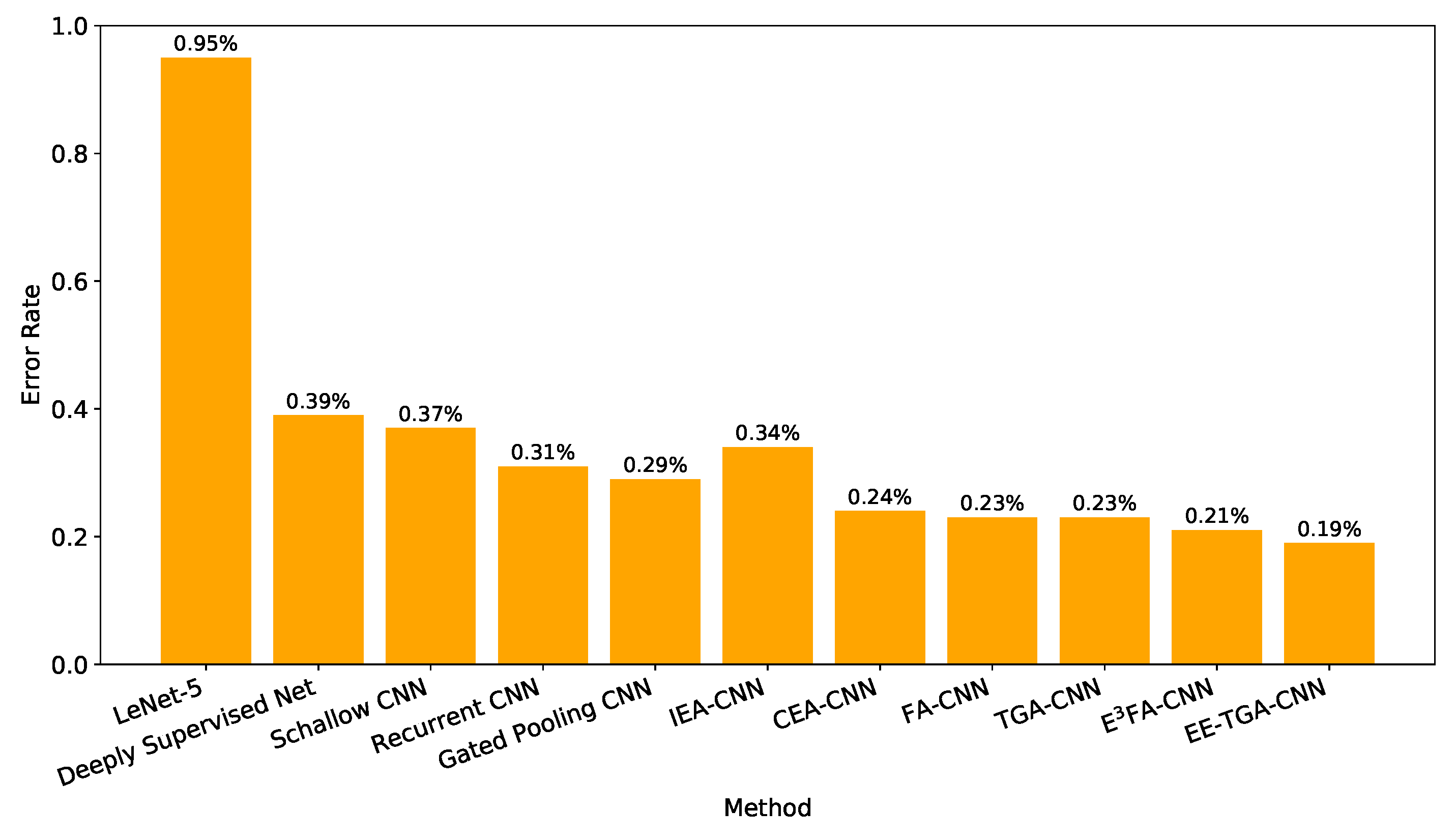
| Method | Test Error Rate (%) |
|---|---|
| LeNet-5 [6] | 0.95 |
| Deeply Supervised Net [83] | 0.39 |
| Shallow CNN [84] | 0.37 |
| Recurrent CNN [85] | 0.31 |
| Gated Pooling CNN [86] | 0.29 |
| IEA-CNN [17] | 0.34 |
| CEA-CNN, k=1 [17] | 0.26 |
| CEA-CNN, k=2 [17] | 0.24 |
| CEA-CNN, k=3 [17] | 0.28 |
| FA-CNN [72] | 0.23 |
| TGA-CNN [71] | 0.23 |
| -FA-CNN | 0.21 |
| EE-TGA-CNN | 0.19 |
© 2020 by the authors. Licensee MDPI, Basel, Switzerland. This article is an open access article distributed under the terms and conditions of the Creative Commons Attribution (CC BY) license (http://creativecommons.org/licenses/by/4.0/).
Share and Cite
Bacanin, N.; Bezdan, T.; Tuba, E.; Strumberger, I.; Tuba, M. Optimizing Convolutional Neural Network Hyperparameters by Enhanced Swarm Intelligence Metaheuristics. Algorithms 2020, 13, 67. https://doi.org/10.3390/a13030067
Bacanin N, Bezdan T, Tuba E, Strumberger I, Tuba M. Optimizing Convolutional Neural Network Hyperparameters by Enhanced Swarm Intelligence Metaheuristics. Algorithms. 2020; 13(3):67. https://doi.org/10.3390/a13030067
Chicago/Turabian StyleBacanin, Nebojsa, Timea Bezdan, Eva Tuba, Ivana Strumberger, and Milan Tuba. 2020. "Optimizing Convolutional Neural Network Hyperparameters by Enhanced Swarm Intelligence Metaheuristics" Algorithms 13, no. 3: 67. https://doi.org/10.3390/a13030067
APA StyleBacanin, N., Bezdan, T., Tuba, E., Strumberger, I., & Tuba, M. (2020). Optimizing Convolutional Neural Network Hyperparameters by Enhanced Swarm Intelligence Metaheuristics. Algorithms, 13(3), 67. https://doi.org/10.3390/a13030067