Abstract
Dynamic Bayesian networks (DBNs) represent complex time-dependent causal relationships through the use of conditional probabilities and directed acyclic graph models. DBNs enable the forward and backward inference of system states, diagnosing current system health, and forecasting future system prognosis within the same modeling framework. As a result, there has been growing interest in using DBNs for reliability engineering problems and applications in risk assessment. However, there are open questions about how they can be used to support diagnostics and prognostic health monitoring of a complex engineering system (CES), e.g., power plants, processing facilities and maritime vessels. These systems’ tightly integrated human, hardware, and software components and dynamic operational environments have previously been difficult to model. As part of the growing literature advancing the understanding of how DBNs can be used to improve the risk assessments and health monitoring of CESs, this paper shows the prognostic and diagnostic inference capabilities that are possible to encapsulate within a single DBN model. Using simulated accident sequence data from a model sodium fast nuclear reactor as a case study, a DBN is designed, quantified, and verified based on evidence associated with a transient overpower. The results indicate that a joint prognostic and diagnostic model that is responsive to new system evidence can be generated from operating data to represent CES health. Such a model can therefore serve as another training tool for CES operators to better prepare for accident scenarios.
1. Introduction
Most industries depend heavily on the functionality of large and costly systems with tightly integrated hardware, software, and human components. Safety risks, financial concerns, and industrial regulations require modeling and predicting the health state of such complex engineering systems (CESs). One modeling framework, dynamic Bayesian networks (DBNs), has shown the ability to infer complex time-dependent causal relationships between nodes connected within these models [1]. As such, there has been growing interest in using DBNs to assess current CES health and model future system health. Applying causal-based reasoning to CES operational data has the potential to generate diagnostic system state models, as well as prognostic outlooks on the future health of the system or potential causes of system failure. However, there are still questions regarding how to make this prognostics and health management (PHM) process effective and efficient for the fast-paced cycle of industry operations and accident sequences.
This paper shows how a DBN model helps provide system health prognostic and diagnostic capabilities for monitoring the health of a CES. Due to the wide range of failure points, components, and data streams that a CES may have, a structured approach is needed to systematically describe and define regions within the model that capture both the CES and the accident scenario space. Using simulated accident sequence data from a transient overpower (TOP) event within a sodium fast nuclear reactor (SFR) as a case study, a joint diagnostic- and prognostic-focused DBN model is constructed from the reactor’s operational data and accident scenario conditions. The output of the model is a posterior estimate for the overall health of the system, the nature of the accident, and potential reactor outcomes.
This paper first discusses the need CESs have for diagnostic and prognostic functions and the challenges that current PHM approaches face when applied to complicated systems (Section 2). An introduction into DBNs and their inference capabilities is then followed by an explanation of how DBNs can be structured around the requirements of CES health monitoring. This framework is then demonstrated through the SFR TOP case study. After the example reactor and accident scenario setups are described, the paper traces the process of constructing a prognostic and diagnostic model for the SFR (Section 3). Model verification results and observations on the model construction process are included in the discussion section, as well as thoughts on future work to improve the model framework’s effectiveness and relevancy to real world systems (Section 4).
2. Materials and Methods
The use of sensors to monitor the health of strategic system components has led to an increase in the availability of data regarding the system’s current performance. These data have the potential to provide diagnostic information about the current health of the overall system, as well as a prognostic assessment of the future state of the system given its current health status. Understanding the current and potential future health states of a system allows its operators and maintainers to make more informed critical operating or maintenance decisions to prolong a system’s operating life before it loses critical functionality. This is a priority for systems that are mission-critical, expensive to repair or replace from a failed state, or pose a safety risk to humans and other associated systems if not fully operable. This process of converting data and expert knowledge from CESs into informed diagnostic and prognostic decisions is illustrated in Figure 1.
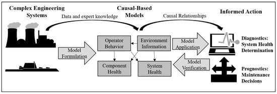
Figure 1.
Modeling complex engineering systems (CESs), such as power plants and large maritime vessels, with causal-based models such as dynamic Bayesian networks, provides system operators and maintainers improved diagnostic and prognostic awareness. This causal knowledge about the system is particularly important following an accident event when action is needed to mitigate system damage and loss of functionality.
Previous PHM research has focused predominantly on smaller components and subsystems. This is in part due to the increased availability of life data for these smaller systems. Additionally, it is easier to assume independence when identifying potential interactions that lead to system or component failure. These prognostic techniques often rely on data coming from a single sensor or sensor type. In his literature review, Guo [2] states that there are three categories for the different approaches to converting system data into a future system health assessment: data-driven, expert-based (often in the form of a physics-based relationship), or a hybrid compilation of the two. Monitoring CES health, however, is more difficult. These systems have multiple integrated hardware, software, and human components functioning together. The subsystems within the platform provide a complicated network of dependencies and common-cause failures. Data from a single data sensor is not sufficient for providing an accurate depiction of system health, and, as a result, prognostic techniques for complex systems require the fusion of data of various types and sources. In their work, Jardine et al. [3] found that data fusion in prognostics takes place in three different approaches based on the data, features, and decisions. Despite these challenges, PHM is an important capability for system operations as many of these CESs are critical to maintain, costly, and potentially harmful if not functioning correctly. This is shown by Muller et al. [4] as their prognosis model was designed to support large industrial maintenance.
Because of the additional hurdles associated with the system health monitoring of complex engineering systems, there have been many different approaches towards generating PHM for complex engineering systems (PACES). An initial approach was identifying relationships within the subsystems and expanding them to the system level. Weber and Jouffe [5] modeled the reliability of complex systems with an object-oriented approach. Over time, PHM strategies continued to incorporate more data from various sources [6]. In 2020, Li et al. [7] created a systematic methodology for defining and designing PHM for aircraft maintenance. While some methods rely on machine learning to take advantage of the large amount of system data available, others adopt a fundamentally different tactic relying on expert knowledge. For example, Zio and Di Maio [8] approached dynamic failure scenarios through fuzzy on-line estimations of the remaining useful life (RUL) of nuclear plants. In these lines of research, the focus was on identifying the future state of the system, rather than diagnosing the current system health.
2.1. Dynamic Bayesian Networks and Related Research
Although there are many manners in which prognostics and overall system health can be assessed for complex systems, the remainder of this paper will focus on one potential modeling method: the dynamic Bayesian network (DBN). Bayesian networks, such as the ones illustrated in Figure 2, are directed acyclical graphs that convey causal relationships through directed arcs between their nodes of associated conditional probabilities [9]. DBNs have been increasingly used in reliability and system safety-related research, as they allow for causal-based inference calculations on hard-to-measure system states while providing a clear direction-based relationship within the structure of the model. The conditional probability tables and initial value distribution used in the networks are calculated from available data or determined through expert-based opinions. Critical to a DBN’s construction is the assumption that future operational conditions are known or stable enough for reliable modeling; works by Djeziri et al. [10] and Mosallam et al. [11] have begun to consider necessary conditions for capturing these missing data.
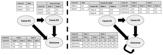
Figure 2.
Sample static Bayesian network (left) and dynamic Bayesian network (DBN) (right). Both models have a relationship structure of nodes and directed arcs as well as conditional probability tables for those relationships; however, dynamic nodes within the DBN also need an initial distribution for their states.
Risk-focused and reliability engineering studies have shown the versatility of these models with respect to system reliability and monitoring system health. Early research connected DBN formalisms to reliability block diagrams [12], dynamic fault trees [13], and Markov chain models [14]. As part of their extensive literature review on the use of Bayesian networks for fault diagnostics, Cai et al. [15] found that more recent research used these fundamental reliability relationships to pursue specific areas of reliability engineering research, including process, structural, and manufacturing systems. Amin et al. [16] used DBNs to determine a dynamic availability assessment of safety critical systems, while Wu [17] found that DBNs could be used to make safety decisions for tunnel constructions. Rebello et al. [18] relied on hidden Markov models (HMMs) to monitor system functionality through DBNs. These researchers wanted to capture the dynamic qualities that would otherwise not be accessible to static models. In addition to the use of DBNs for system diagnostic purposes, there has been some research into whether this method could be used for prognostics as well. Medjaher et al. [19] represented a small industrial system through DBNs to determine the expected prognostics of the system. Zhao et al. [20] proposed the use of DBNs to monitor fault diagnostics and loss-of-coolant accident progression prediction in a high-temperature gas-cooled reactor pebble-bed module (HTR-PM) reactor. In each of these instances, an emphasis was placed either on the system health prognostics or diagnostics of the system; there has been limited effort made to combine this information into a single model.
DBNs are also used in modeling for risk management of systems. Initial research by Kohda and Cui [21] found that DBNs could be applied to a safety monitoring system to improve its capabilities. Khakzad [22,23] has shown the applicability of DBNs in capturing performance assessments in fires in chemical plants. Groth et al. [1] have used DBNs as part of a process for providing risk-informed diagnosis procedures. However, there has not been a significant push to merge risk-informed dynamic Bayesian models with the system health of a complex engineering system to generate insight into the current health of the system.
2.2. Using Dynamic Bayesian Networks to Model Complex Engineering Systems
One of the primary characteristics of Bayesian networks and other causal-based models heavily used in previous research efforts is that evidence concerning the state of one node can lead to an updated estimate of the value of another node within the model through logical inferences. The ability to infer the status of nodes within a dynamic Bayesian network translates into a powerful tool for understanding the current health condition of a system. DBN nodes can represent a wide range of features within a system, from individual sensors to entire subsystems. As inference capabilities are associated with the directed arcs between nodes, i.e., the node relationships, information about the system can act as evidence in one section of the model, which then travels to other parts of the model. This allows the DBN model to utilize more evidence and provide more insight into the system than otherwise expected. The dynamic aspect of DBNs is the repeated occurrence of evidence for the same node. For this case study, and in most instances, DBNs are characterized as a two-time-step model, in which the current node values are only related to the immediate time step beforehand. This Markov structure, therefore, suggests that for a given Bayesian network with variables, the underlying probability that a certain scenario would occur, P, is based on Equation (1) from Cai et al. [15]:
where is the set of nodes with arcs into the variable . This may not hold for networks that have more complicated time-based ordering; however, this assumption is often used for the ease of modeling dynamic relationships.
Since inference generated within a DBN can run from parent to child nodes and vice versa, information from separate parts of the model can provide information to other aspects; for a CES, this widens the range of information available for use. As a result, DBN models designed to monitor CES health can have nodes for sensors, components or subsystems that a) either provide useful or readily available data for use as system evidence, or b) are aspects of the CES that operators and maintainers would want to know information about. Consider the theoretical DBN shown in Figure 3. Information provided about an operator’s behavior or the system’s environment may change the expected state of a specific component’s or the system’s overall health.
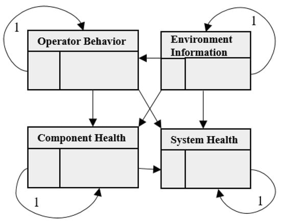
Figure 3.
Theoretical DBN construct that indicates the relationships between event/accident data, system information from sensor data, the overall system diagnostics, and prognostics. Additional information about each node could then be used to infer posterior estimates of the other nodes.
A DBN model designed to monitor and provide information on the health state of a CES following a major accident should incorporate not only operational system information, but also the conditions of potential accidents. As shown in Figure 4, DBN models representing this CES scenario can be structured using four distinct data regions. Each section of the model has its own node types, data availability, and purpose for managing CES health. These four regions are:
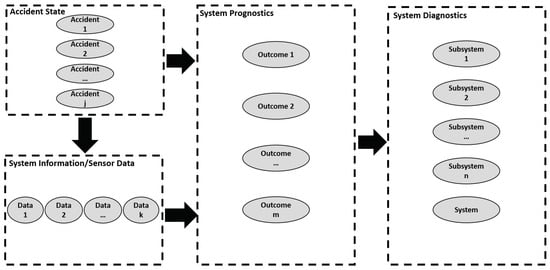
Figure 4.
The nodes within a DBN model designed to monitor CES health following an accident event can be classified into four information regions: accident state, system information and sensor data, system prognostics, and system diagnostics. The arrows drawn between the information regions reflect the directed relationships; the model is designed so that each node is fully connected to the child information region (i.e., each “Accident State” node is fully connected to every “System Information/Sensor Data” node and every “System Prognostics” node).
- Accident State: the nodes within this region represent the different accident events the system might encounter that this model covers. Typically, CESs are operating at normal or baseline conditions until one of these events occur; after an accident, the system will be operating under different circumstances. The type of accidents that this model covers may be either external to the system (i.e., an earthquake or a power outage) or internal (sabotage). Depending on the potential accidents that may impact the CES, different accident nodes will be needed to reflect different states that may not be mutually exclusive and occur at the same time;
- System Information/Sensor Data: CESs generate a sizable amount of data of different types and in varying frequencies. These data can take the form of sensor readings, analytical measurements, and status and maintenance reports, and can either be continuous or discrete. Since data sources are frequently updated with new system information, these are the “dynamic” nodes of the DBN. The classification of data into discrete bins is dependent upon the nature of the data; however, a common bin distribution would be for “normal operating conditions”, “above operating conditions”, and “below operating conditions”. This region is predominantly where additional model evidence is added to the DBN, as extra information can be used to make informed decisions about the nodes in the other regions;
- System Prognostics: this region of the model provides insight into potential failure modes that a CES might fail from given a particular accident. These are typically distinct from other prognostics techniques, which might indicate a remaining useful life of the system; rather than indicating whether a system will be healthy or faulty at a given point in time, these nodes indicate what will be the resulting failure of the system given the current system information and data. Examples may include “metal cladding failure” or “short-circuit” and are often expressed as a binary option (i.e., “Yes/True” and “No/False”). Each failure event state should be considered as a separate node;
- System Diagnostics: Based on the system prognostics estimate captured in the “System Prognostics” region, CES health can be assessed by whether or not the system will fail from another failure mode other than expected failures at the end of its life cycle. Unlike the other nodes, this region can be fully captured in a single node with a number of mutually exclusive states; depending on the CES’s structure, this approach can be used on the subsystem level as well. An easy way of expressing this is through a simple OR gate-style node for overall system health. Examples of states may include “Healthy”, “Faulty”, or “Inoperable”.
Following Figure 4, information about the accident state as well as system or sensor data provide information about the current system diagnostics. An understanding of the current system health in conjunction with the system measurements can be used for system prognostics to identify potential causes of system failure. Because of the relationship arcs connecting the four different regions within a DBN, a model structured in this manner can be used to provide diagnostics and prognostics. From the information provided by the sensor and an understanding about the accident sequences, understanding about the current health of the system can be determined. Using the time-dependent relationships of each system as well, that information can be propagated backwards to adjust understanding of the system. This will in turn adjust the current understanding. Similar to diagnostics, a predictive end state can be introduced into a DBN. The benefit of including this in a temporal network is that the probability of certain prognostic updates can fluctuate, and these can then be used to make a prediction over the state of the system. Information provided about the current system can then be used to calculate the future outcomes that the system might face.
This structure of system data and model evidence into these distinct information regions is scalable to address the different accidents, data types, and prognostics failure modes. It is also compressible: a purely prognostics-focused model can have the failure state nodes act as root nodes, while a solely diagnostics model would have a singular failure mode in the system prognostics information region: “Failure”. In that case, the resulting diagnostics node would simply duplicate the probabilities calculated for the prognostic node; it acts as an identity node for the binary failure state.
2.3. Case Study: Transient Overpower Event (TOP) in a Sodium Fast Reactor (SFR)
In order to show how such a DBN structure can be used to provide joint prognostics and diagnostic capabilities aimed at assessing CES health and their potential failures following an accident event, the remainder of this paper will present a sample DBN for modeling and monitoring an SFR reactor in a transient overpower event. This case study is a simplified exercise conducted by Groth et al. [1] with the data modifications made by Jankovsky et al. [24]. This section will begin with a description of both the SFR and the TOP scenario that the model is designed to monitor. The construction of the model is then discussed. Results from the model will then be used to illustrate the additional prognostic and diagnostic capabilities that DBNs can provide for complicated systems and processes with multiple integrated parts. These sections are written as a fairly high overview; further details regarding the accident dataset and the overall DBN construction process are covered in Appendix A and Appendix B, respectively.
2.3.1. Case Study Background—Reactor and Accident Description
For this case study, a Sodium Fast Reactor (SFR) will serve as a typical complex engineering system. As these type of reactors rely on fast-neutron activity, the need for other equipment is minimized, making them useful models for complicated nuclear reactions. In addition to the nuclear core, the system has a balance of plant and an auxiliary cooling process; however, for this demonstration, the focus will be on the reactor core itself. Although there are multiple components to a sodium fast reactor that provide a significant amount of system information through sensors and operational reports, this initial study will focus on a limited number of data sources, namely the primary drivers for the automatic scramming process to shut down reactor power.
In this case study, the primary accident event described through the DBN model is a transient overpower (TOP) event. Such an event can be caused by external factors, e.g., an earthquake, that result in a sudden surge of power generation in the reactor. When such an event occurs, the reactor’s automatic scram mechanism is expected to respond by inserting control rods into the reactor to greatly reduce power generation; common indicators for the automatic scram mechanism include large power-to-flow readings, as well as high values of reactor pressure, inlet, and outlet temperature [24]. Depending on the cause of the accident, however, scram functions may be impacted, limiting their ability to prevent core reactions from further escalating. If this were to occur, the reactor would face significant failure challenges with fuel relocation and clad melting, resulting in a partial or full nuclear meltdown.
The accident data used in this case study is from the study by Jankovsky et al. [24]. In their report, a series of accident event scenarios were constructed using a dynamic event tree that addressed potential failure points in response to the TOP. Based on the event scenario specifications, simulation models focusing on different aspects of the nuclear reactor were used to produce different parameters necessary for monitoring overall system health. The models were run to simulate data readings throughout the reactor and balance of plant a day after a transient overpower event (86,400 simulation seconds). The scenario was considered finished when either: the cladding fraction of the core channels reached an average of 90% (representing a clad melting failure); the temperature of the cold pool had reached a significantly high temperature (representing a fuel relocation); or the reactor had survived the day without reaching those other thresholds. In that instance, it is assumed that operators would have enough time to address any problems with the system’s processes.
Three datasets captured different parameters that could be used to provide system operational data. They provided information about the reactor channels, overall reaction values, and information about the balance of plant and auxiliary systems. These datasets were created from the following two models:
- SAS4A/SASSYS-1: this code provides information about the nuclear reactions occurring within the four channels of the reactor. Data provided from this part include inlet and outlet temperature and inlet and outlet flow. Additionally, the model was used to generate any current nuclear core activities, such as power generation and reaction coefficient values. These model data provide insight into the current power generated from the reactor and other information about physical nuclear reaction;
- PRIMAR4: this simulation code generates values for the overall piping and thermodynamics of the system, including the balance of plant and other auxiliary systems. This includes information about the temperature and pressures of compressible volumes and pools around the reactor, measurements of the pumps and the different elements of the balance of plant and cooling systems.
From these models, an operational timeline can be comprised of the different parameters necessary for monitoring overall system health.
2.3.2. DBN Construction
For this study, a simplified model was constructed to cover the primary elements of the SFR that are relevant for scramming failures in the event of a transient overpower. As previously mentioned, automatic scram action occurs when the power-to-flow ratio, the reactor’s inlet and outlet temperature, or overall reactor pressure are measured above a certain threshold. Designing a DBN model to help operators identify current system health status and potential failure modes, as shown in Figure 5, therefore requires nodes in the accident state, system and sensor information, system diagnostics, and system prognostics information regions. The temporal loops included for the system information nodes (Power-to-flow, Pressure, Inlet and Outlet Temperature) indicate a distinct dependency on previous parameter values, unlike the other nodes which have static conditional probabilities (i.e., a prediction of the current scram state is not dependent upon the scram state prediction from a previous measurement). This model’s conditional probability tables are trained with operational data provided from scenarios that resulted in three distinct outcomes: failure due to clad melting; failure due to thermal relocation; and a successful model outcome. The model’s objective is identifying the current health state of the reactor as well as the likelihood of a certain outcome based on current data from the system’s sensors. Data received from the system will be used as evidence for an improved determination of the state of the reactor’s scram and trip mechanism. The DBN model is constructed using the GeNIE software; conditional probability table (CPT) elements are calculated using the Python programming language.
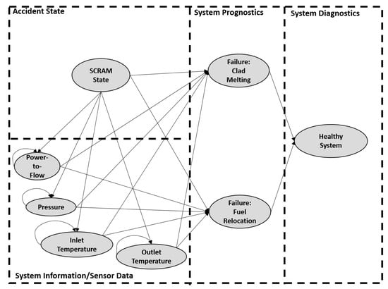
Figure 5.
DBN node structure and relationship graph for the SFR transient overpower (TOP) case study. The dashed boxes represent the different node regions for a diagnostics and prognostics model for CES. The arrows are reflective on the current time step, with the exception of the dynamic relationship in the nodes in the “System Information/Sensor Data” box.
As CESs generate a multitude of data, there are large amounts of readily available data that can be used to inform the model’s quantification of the conditional probability tables. The information provided for this model was carried out in multiple simulations over different time period measurements. For example, nuclear reactor data from the SAS4A-SASSYS-1 code was collected more rapidly at the beginning of the accident simulation, at a rate of 0.1 simulation seconds, and slowed down to a collection frequency of 100 s. On the other hand, new information from the PRIMAR4 code was provided approximately every nine seconds. This is similar to real-world scenarios in which measurements and sensor readings occur over different frequencies. As such, operators are dealing with a mixture of newer and older information and need to consider these respectively. In order to capture as much relevant information as possible, an operational timeline was created to consolidate both model readings into one sequence of events. As illustrated in Figure 6, relevant information was identified from both models. The available data were then sorted based on the simulation time at which the data were received. When new data were acquired from a sensor, that entry would replace the measurement from the previous timing; however, the “current” information from other system sensors would remain as new data have not yet been provided.
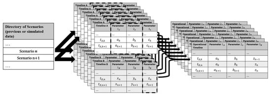
Figure 6.
Data from different models with varying time frequencies are compiled into a single operational timeline. Given multiple accident scenarios, this produces many example operational timelines, which can be used for constructing the DBN’s conditional probability tables.
Using the simulated data generated from the reactor and infrastructure models, a sample set of conditional probability tables, which reflects how the health of the nuclear reactor system progresses over time, was quantified. The CPTs provide insight into the transformation of the different nodes across the model and describe the causal relationships within the nodes. For this DBN structure, there are three types of CPT that are reflective of different structures in the nodes: static CPTs for the static nodes and initialization and temporal CPTs for the dynamic nodes. For these CPTs, the elements in the table can be determined by a frequentist approach by counting the number of instances a child node state occurred with the identified parent node states, or
DBN nodes are designed to contain discrete states; for this model, the simulation data provided were separated into ranges based on reasonable expectations for “Low”, “Medium”, or “High” values. These determinations were based on what is expected either through expert opinion or a collection of information. For this case study, information from a simulated scenario in which no TOP occurred was used as a baseline for what would fall in the middle bin. Bin discretizations vary based on the data that the model is relying on, but the example ranges are shown in Table 1.

Table 1.
Model parameters and discretized bin threshold values based on baseline operational data.
Dynamic nodes within the DBN require an initial distribution for their states, from which the temporal conditions rely on, for the proceeding time steps. For this study, it is assumed, unless evidence is provided otherwise, that the initial state of the system is healthy and running at a normal operational status as expected from the baseline operations.
3. Results
Based on the previous model and data received, the CPTs for the previously described model were quantified. Where there was evidence, a frequentist approach of determining probabilities was used; however, when that data was not available, appropriate approximations were used to complete the table that would minimize influencing the posterior estimates to a greater extent than the available information. Table 2 is an example of one of the quantified dynamic CPTs. In each instance, the majority of data was classified in the same bin as the previous measurement; any deviation would therefore be considered a rare event and worth noting. Although certain relationships might not occur in an actual accident scenario, those elements still need to be included in the CPTs.
Table 2.
Dynamic conditional probability table (CPT) for CV1 Pressure Measurements. Note the columns with the round estimates (expert-based opinions) interspersed with the more precise estimates based on the available data.
To show the model’s effectiveness at assessing an SFR’s health state following an accident event and potential future failure outcomes, hypothetical data are provided to the model that may be indicative of a TOP. These data will serve as evidence, which will impact the posterior estimates for the system prognostics, diagnostics, and accident state.
A transient overpower could be initially indicated by an increase in the power-to-flow ratio. Table 3 shows the prior and posterior scram state probabilities with evidence that the power-to-flow ratio was found to be higher than a baseline amount and all other relevant parameters were held the same. As expected, the prior probabilities of the scram state and the power-to-flow CPTs along with the limited amount of information provided little change to the prior; this model is still predominantly assessing that the scram process is working as intended. Although minute, the posterior estimates for the state of the scram and trip mechanisms are changing. However, just as in most instances, that information alone is not enough to convince the model that something is seriously going wrong. There are many reasons that the power-to-flow ratio may be higher than baseline measurements; given the significantly low probability that the scram and trip mechanism fails, the model is estimating that there is something else that could explain the discrepancy. This is also seen in the system prognostics at this particular point in time, as shown in Table 4. For both instances, the probability of failure is either non-existent or negligible.
Table 3.
Prior and posterior probabilities of scram, prognostics, and system diagnostics with evidence of high power-to-flow ratio.
Table 4.
Prognostics outcome for reactor with high power-to-flow reading.
This assessment of the reactor’s prognostics changes, however, when new information is received. Assume now that the following sensor readings indicate that not only is the power-to-flow value still above the operational baseline, but the outlet temperature of the reactor is also higher than anticipated. This is then followed by another reading of high power-to-flow and outlet and inlet temperatures. This combination of evidence, in addition to the initial high power-to-flow value, significantly alters the estimate of whether the scramming mechanism worked, as seen in Table 5. The posterior estimates indicate that it is more likely that the scram and trip failed. The model responds to a small amount of information to raise a concern that an accident has indeed occurred.
Table 5.
Prior and posterior probabilities of scram, prognostics, and system diagnostics based on the listed evidence.
The addition of new data also changed the current prognostics outlook of the system, as seen in Table 6. The previous prognostics seen in Table 4 showed a negligible reactor failure from clad melting, and a nonexistent risk from fuel relocation; however, that assessment was based on the assumption that the scram and trip mechanism were successful. Since the new evidence introduced into the model changed the posterior estimate of the scram state to have failed in some manner, there is a greater likelihood that the reactor will fail by one of those failure modes. The updated prognostics now suggest that given the current data received from the system sensors, there is a 0.31% chance that the system, if conditions remain the same, would result in a failure by fuel relocation. Interestingly, the probability that the system would fail from clad melting has been reduced. These two facts are the result of the specific conditional probability tables used to project sensor measurement values. This assessment does match expected results, as both clad melting and fuel relocation occur when outlet temperatures are hotter than operation levels; however, fuel relocation can occur faster at higher reactor temperatures.
Table 6.
Prognostic outcome for reactor with high power-to-flow reading, followed by high power-to-flow and outlet temperature readings, and then high power-to-flow, outlet and inlet temperature measurements at Time 3.
In addition to changing the assessment of the reactor’s prognostics, the influx of new system data and sensor information should impact the estimate of the reactor’s health. Table 7 provides point estimates on the reactor system’s diagnostics. At the beginning of the experiment (Time 0), there is no indication that the system would be faulty as the initial state distribution is consistent with that of the operating baseline; as a result, it is deemed a fully healthy system. When the high power-to-flow measurement comes in at Time 1, there is now a possibility that one of the failure outcomes could occur; as a result, the reactor’s health is marginally diminished. When the additional power-to-flow and outlet temperature data are received at Time 2, and it becomes evident to the model that a failure in the scram mechanism has occurred, the system’s health diagnostic assessment is significantly degraded. The collection of this result, as well as the prognostic assessments and estimate in scram failure, would result in a more educated process to find and address the issue, minimizing any potentially harmful outcomes.
Table 7.
Progression of system diagnostics following the example accident sequence.
4. Discussion
The results indicate that the DBN model provided a system diagnostic and prognostic capability for the reactor accident sequences that it was designed to monitor. Using available information from a large number of system sensors, a clearer image of the current and future system health was estimated for a complex system. The strength of the model lies in its inference abilities, as it provides a responsive posterior probability for both specific system outcomes and current health and accident states. This type of modeling is important to consider when monitoring CES health, as it provides a visually appealing method of presenting the causal relationships found in these systems and subsystems. CESs have heavily integrated platforms that, through other techniques, would otherwise not have their time-dependent causal relationships truly defined. As this capability is possible with DBN models, there are now better and more accurate PHM strategies that are available to use on CESs than previously utilized.
One of the common challenges associated with applying DBNs to real systems is the CPT quantification process. Depending on the number of state bins and the amount of parents for each node, the size of the tables can vary greatly, increasing the time and power required to process the probabilities. For this case study, most failure scenarios led to the same parent/child node relationships and some parent/child combinations were not met. Limiting the number of accident scenarios, minimizing the amount of states per node, and relying on expert-based relationships may reduce the computational requirements; however, an increase in the number of scenarios and state bins make the model applicable to a wider range of accidents and failure modes and increases the granularity of the model, respectively. An analysis is needed to identify the proper amount of granularity and model coverage for each specific CES.
The current structure of the DBN model is designed for a continuously operating CES that can experience an accident at any given moment. Given the long operational lifetime of these systems relative to the start-up and wind-down time periods, this is a reasonable assumption; however, accidents can just as easily occur at the onset of operation or operation build-up. To consider these time periods when constructing a model, data or expert-based opinions of the system relationships are needed. Such a model may end up entirely distinct from one of a similar CES in its operational phase.
As this modeling approach is intended to work for all CESs that experience accident events, there are many areas of improvement for this type of work to reflect the diversity of its application areas:
- First, further study is needed on the impact that the time step measurements at which data are received have on CES prognostics and diagnostics assessments. In the SFR case study, the CPTs were designed with data collected over varying lengths of time but assumed to be equal evidence. Constructing the CPTs over simulation time, rather than data collection time, may result in a different assessment of system health. An initial study by Lewis and Groth looked at the potential impacts that different time discretization techniques had on prognostics and diagnostics performance. The SFR case study could be used as a case study to quantify some of these differences [25];
- One major assumption in constructing the operational timelines for different accident scenarios was that every piece of system information not received at that point in time was assumed to be constant until otherwise changed. Additional work is needed to identify other methods of unmeasured system data evolution, as it is possible that other predictive approaches, such as filtering or forecasting, may ultimately be used to provide a more accurate estimate of certain values before the new values become known;
- Another set of assumptions present in the case study was the number of expert opinions used to fill the conditional probability tables for events and conditions that did not have available data. The current DBN structure itself is not able to fully incorporate physical knowledge of the system, such as degradation and failure modes, into its diagnostic and prognostic assessments; as such, this system information might be a better alternative for substituting missing data with respect to nodes related to remaining useful life predictions. There has been a range of work in this subject for various systems, including wind turbines [26], railways [27], and subsea pipelines [28];
- A next-level line of study would be to vary the weight of information provided to the system as evidence. Currently, all information used by the model carries the same weight. Certain sensor readings may be more reliable or provide a greater amount of evidence than other sensors; newer system information should take greater precedence in system health assessments than older information;
- Another area worth addressing is the bin size for each of the nodes, particularly those in the system data and system information region. Since the conditional probability tables are dependent upon where state bin thresholds are located, adjusting the bin boundaries will have a significant impact on the conditional probability tables that the model is dependent on. Previous work by Zhu and Collette [29] has found attempts to discretize the bins dynamically. This study would also be associated with identifying the appropriate number of bins, based on the findings from Yang and Webb [30]. As an increase in bins allows a greater number of variations, the logical extension of this would be aligned with some of the research that Li et al. [31], Codetta-Raiteri et al. [32], or Iamsumang et al. [33] have performed on continuous-time or hybrid Bayesian networks. Future research from Codetta-Raiteri [32] has even suggested creating a continuous-time-based DBN that provides insight over conditional states that are not discrete but based on continuous probabilistic distributions;
- Lastly, a more complicated model could be created by introducing additional accident states to the CES. Having an additional accident state would result in different parameters having different relationships with the same or other relevant system data. Further research is needed to determine how those can be successfully integrated into the model.
The direction of where DBN modeling for CES prognostics and diagnostics is heading depends on the priority of the researchers in each application area. Understanding any one of these incomplete research areas better, however, will result in a diagnostic and prognostic model that better reflects the requirement of the CES.
5. Conclusions
This paper shows how a DBN structure could be used for a joint diagnostic and prognostic model for monitoring complex engineering system health following an accident event. By breaking apart the model nodes into four distinct information regions, access to sensor data and system information allow for different assessments for accident scenarios, prognostics, and diagnostics for systems and subsystems. Through the SFR TOP case study, expert-based opinions and data-driven techniques were used to quantify the DBN’s CPTs and strengthen the model. The model responded to the hypothetical accident data supplied as evidence by indicating an increased chance of scram and trip mechanism failure and overall system failure, and a decrease in overall system health. Such an ability suggests that this model can be used to prepare CES operators for rare-event accident scenarios. Potential extensions of the current work may include applying the model structure to other CES accident scenarios, fine-tuning the model design and construction process, or studying a multi-accident scenario sequence.
Author Contributions
A.D.L. and K.M.G. contributed to conceptualization, methodology, and visualization; A.D.L. contributed software, formal analysis, data curation, and writing—original draft preparation; K.M.G. contributed supervision, project administration, funding acquisition, and writing—review and editing. All authors have read and agreed to the published version of the manuscript.
Funding
This research was funded in part by the University of Maryland, including the Clark Doctoral Fellowship Program at the University of Maryland. Writing was supported under award 31310018M0043 from the U.S. Nuclear Regulatory Commission. The statements, findings, conclusions, and recommendations are those of the authors and do not necessarily reflect the view of the U.S. Nuclear Regulatory Commission.
Conflicts of Interest
The authors declare no conflict of interest. The funders had no role in the design of the study; in the collection, analyses, or interpretation of data; in the writing of the manuscript, or in the decision to publish the results.
Abbreviations
The following abbreviations are used in this manuscript:
| CES | Complex engineering system |
| CPT | Conditional probability table |
| DBN | Dynamic Bayesian network |
| DET | Dynamic event trees |
| PACES | PHM approaches to complex engineering systems |
| PHM | Prognostics and health management |
| PSID | Preliminary safety information document |
| RUL | Remaining useful life |
| SFR | Sodium fast reactor |
| TOP | Transient overpower |
Appendix A. Case Study Data
The data used in this case study are the result of simulations run by Jankovsky et al. [24] using the SAS4A/SASSYS-1 and PRIMAR4 models as part of a project to develop methodologies for merging dynamic event trees (DETs) with operator actions. The dynamic event tree was designed to “investigate the effects of various mitigating actions and uncertain plant parameters in an SFR following an inadvertent insertion of reactivity”. It consisted of seven branching conditions and two ending conditions that had two to ten child branches each. This resulted in a collection of 2052 accident sequences that had the outcomes of model success, clad relocation, or temperature failure. A SAS4A/SASSYS-1 model was then used to calculate the data along the tree.
For this case study, only one branching condition and its relation to the scenario outcome was considered (Scram and Trip Success).
Appendix B. Case Study DBN Formation
This appendix describes the formation of the DBN for the case study scenario of a sodium fast reactor experiencing a scramming mechanism failure during a transient overpower.
Appendix B.1. Overview
Figure A1 is the illustration of the DBN model nodes and directed relationships within their respective information regions. This network structure was determined by a general understanding of the nature of the scramming mechanism and the two described failure modes in the study by Jankovsky, et al. [24]. Table A1 lists the nodes constructed in the model, the information region they are located in, and the number and the value of node states.

Figure A1.
DBN node structure and relationship graph for the SFR TOP case study. The dashed boxes represent the different node regions for the diagnostics and prognostics model for CES. The arrows are reflective on the current time step, with the exception of the dynamic relationship in the nodes in the “System Information/Sensor Data” box.

Table A1.
Model nodes and node states.
Table A1.
Model nodes and node states.
| Node Name | Type of Node | Number of States | General State Descriptions |
|---|---|---|---|
| Scram State | Accident State | 4 | Scram and Trip Success, |
| Scram Success and Trip Failure, | |||
| Scram Failure and Trip Success, | |||
| Scram and Trip Failure | |||
| Inlet Temperature | System Information/Sensor Data | 3 | Low, Medium, High |
| Outlet Temperature | System Information/Sensor Data | 3 | Low, Medium, High |
| Power-to-Flow | System Information/Sensor Data | 3 | Low, Medium, High |
| Pressure | System Information/Sensor Data | 3 | Low, Medium, High |
| Failure: Thermal Melting | System Prognostics | 2 | Yes, No |
| Failure: Clad Fraction | System Prognostics | 2 | Yes, No |
| System Diagnostics | System Diagnostics | 2 | Yes, No |
In addition to a network structure of nodes and directed arcs, a DBN model requires associated conditional probability tables, as well as an additional initial distribution table for the dynamically changing nodes. Therefore, the following is the list of CPT tables needed for the model designed for the SFR scenario:
- Static Conditional Probability Tables
- ;
- ;
- ;
- ;
- ;
- ;
- ;
- .
- Dynamic Conditional Probability Tables
- ;
- ;
- ;
- .
To quantify these tables, either prior expert knowledge or operational data are required. For this case study, a hybrid approach was used to complete the CPTs. Expert-based opinions were determined from either source documents (i.e., the preliminary safety information document (PSID)) [34], or were mentioned in the study by Jankovsky et al. [24]. The operational data used were received from Sandia National Laboratories.
Appendix B.2. Coding Scenario Information
The structure of the model relies on data from both system sensors and other monitoring equipment, in addition to situational information regarding different accident scenarios that the reactor may be exposed to. The scenario information describes the different conditions following the accident event as well as the simulated outcome of that particular event sequence (successful system survival or system failure). To allow the DBN model’s CPTs to be constructed from the operational data attached to the different scenario sequences, data measurements from the different system parameters (Power-to-Flow, Inlet and Outlet Temperature, CV1 Pressure) were assigned a number based on the amount of bins available for discretization. For this study, the sensor data were treated with either “High”, “Medium/Normal”, or “Low” relative to baseline operating information.
Appendix B.3. Creating Operational Timelines for Different Timelines
In order to create the conditional probability tables for each of the nodes, the operational data is formatted into a single timeline. Relevant information was identified from both models; in the case study, the system sensors were the primary indicators for the automatic scram and trip mechanism. Those two data sets were then merged together and sorted based on the timing that the information was received. In some instances, data from one model was received, and not from the other. In those instances, the newer information replaces the earlier measurements received from the same system sensor, whereas all other system information remains the same.
Appendix B.4. Separating Scenario Outcomes by Accident Node State (Scram State)
Based on the model structure shown in Figure A1, the accident node “SCRAM state” is connected to each of the system information/sensor data as well as to the system prognostic nodes; as a result, it is important to be able to classify the accident scenario sequences by their accident states. This requires the operational data to be categorized according to what accident the reactor experienced. This situational information is critical for constructing the CPTs for the CES prognostics nodes.
Appendix B.5. Creating the CPTs
The conditional probability tables for each node were created by measuring the frequency of different data combinations with respect to the different node states and supplementing the available data with expert opinions when there was no information available. For example, for the dynamic table for the inlet temperature, the value was calculated for the different values of inlet temperatures that were associated with each of the different scram/trip states and previous values. Each state was then normalized over the same parent node conditions.
The manner of providing expert opinion for the CPTs depended on the nature of the CPTs as well as the location of the node:
- Accident State (Scram State): The expert opinion used to construct the CPT for the “Scram State” node was based on probabilities taken from the PRISM preliminary safety information document (PSID) and listed in Table A2 [34]:
Table A2.
Prior distribution for SCRAM state.
Table A2.
Prior distribution for SCRAM state.
| Scram State | Prior Distribution |
|---|---|
| Scram and Trip Success | |
| Scram Success and Trip Failure | |
| Scram Failure and Trip Success | |
| Scram and Trip Failure |
- System Information/Sensor Data (Inlet Temperature, Outlet Temperature, Power-to-Flow Ratio, Pressure near Inlet): The initial distribution of each measurement was assumed to be within the normal operating baseline of the variable; therefore, the initial measurement for each system sensor started in the middle bin marked “Medium/Normal”. For the dynamic distributions, the conditional probabilities were dependent on the sensor values in the previous time period; as a result, CPTs that were missing a parent node condition would substitute the blank column with one of the following listed in Table A3:
Table A3.
Filled-in columns for missing information in case study dynamic conditional probability table.
Table A3.
Filled-in columns for missing information in case study dynamic conditional probability table.
| System Information/Sensor Data | Dynamic CPT | ||
|---|---|---|---|
| Scram State | Scram State [i] | ||
| (Self) | Low | Middle | High |
| Low | 0.9 | 0.05 | 0 |
| Middle | 0.1 | 0.9 | 0.1 |
| High | 0 | 0.05 | 0.9 |
- System Prognostics (Failure: Fuel Relocation, Failure: Clad Melting): Because of the limited number of scenarios that result in an overall system failure from the two outcomes specified in the case study, the prognostics CPTs are the most incomplete in the model. To fill the CPTs with values that would not skew the outcome, it was assumed that the empty parent condition cases would result in a 1:1000 chance of having either system failure occur;
- System Diagnostics (Diagnostics): For this model, it is assumed that if a failure occurs, then the system is not healthy. As such, the CPT for the diagnostics node “Diagnostics” is constructed using the conditional probability table shown in Table A4:
Table A4.
Conditional probability table for diagnostics node.
Table A4.
Conditional probability table for diagnostics node.
| Diagnostics | Distribution | |||
|---|---|---|---|---|
| Failure: Fuel Relocation | True | False | ||
| Failure: Clad Melting | True | False | True | False |
| Healthy | 0 | 0 | 0 | 1 |
| Not Healthy | 1 | 1 | 1 | 0 |
References
- Groth, K.; Denman, M.; Darling, M.; Jones, T.; Luger, G. Building and using dynamic risk-informed diagnosis procedures for complex system accidents. Proc. Inst. Mech. Eng. O-J. Ris. 2020, 3, 193–207. [Google Scholar] [CrossRef]
- Guo, J.; Li, Z.; Li, M. A Review on Prognostics Methods for Engineering Systems. IEEE Trans. Reliab. 2019, 99, 1–20. [Google Scholar] [CrossRef]
- Jardine, A.K.; Lin, D.; Banjevic, D. A review on machinery diagnostics and prognostics implementing condition-based maintenance. Mech. Syst. Signal Process. 2006, 20, 1483–1510. [Google Scholar] [CrossRef]
- Muller, A.; Suhner, M.C.; Iung, B. Formalisation of a new prognosis model for supporting proactive maintenance implementation on industrial system. Reliab. Eng. Syst. Saf. 2008, 93, 234–253. [Google Scholar] [CrossRef]
- Weber, P.; Jouffe, L. Complex system reliability modelling with dynamic object oriented Bayesian networks (DOOBN). Reliab. Eng. Syst. Saf. 2006, 91, 149–162. [Google Scholar] [CrossRef]
- Guillén, A.J.; Gómez, J.F.; Crespo, A.; Guerrerro, A.; Sola, A.; Barbera, L. Advances in PHM application frameworks: Processing methods, prognosis models, decision making. Chem. Eng. 2013, 33, 391–396. [Google Scholar]
- Li, R.; Verhagen, W.J.; Curran, R. A systematic methodology for Prognostic and Health Management system architecture definition. Reliab. Eng. Syst. Saf. 2020, 193, 106598. [Google Scholar] [CrossRef]
- Zio, E.; Di Maio, F. A data-driven fuzzy approach for predicting the remaining useful life in dynamic failure scenarios of a nuclear system. Reliab. Eng. Syst. Saf. 2010, 95, 49–57. [Google Scholar] [CrossRef]
- Dean, T.; Kanazawa, K. A model for reasoning about persistence and causation. Comput. Intell. 1989, 5, 142–150. [Google Scholar] [CrossRef]
- Djeziri, M.; Benmoussa, S.; Benbouzid, M.E. Data-driven approach augmented in simulation for robust fault prognosis. Eng. Appl. Artif. Intell. 2019, 86, 154–164. [Google Scholar] [CrossRef]
- Mosallam, A.; Medjaher, K.; Zerhouni, N. Data-driven prognostic method based on Bayesian approaches for direct remaining useful life prediction. J. Intell. Manuf. 2016, 27, 1037–1048. [Google Scholar] [CrossRef]
- Torres-Toledano, J.G.; Sucar, L.E. Bayesian networks for reliability analysis of complex systems. In Progress in Artificial Intelligence–IBERAMIA 98; Coelho, H., Ed.; Springer: Berlin, Germany, 1998; Volume 1484, pp. 195–206. [Google Scholar]
- Boudali, H.; Dugan, J.B. A discrete-time Bayesian network reliability modeling and analysis framework. Reliab. Eng. Syst. Saf. 2005, 87, 337–349. [Google Scholar] [CrossRef]
- Weber, P.; Jouffe, L. Reliability modelling with dynamic bayesian networks. In Proceedings of the 5th IFAC Symposium on Fault Detection, Supervision and Safety of Technical Processes 2003, Wahsington, DC, USA, 9–11 June 2003; Volume 36, pp. 57–62. [Google Scholar]
- Cai, B.; Huang, L.; Xie, M. Bayesian networks in fault diagnosis. IEEE Trans. Industr. Inform. 2017, 13, 2227–2240. [Google Scholar] [CrossRef]
- Amin, M.T.; Khan, F.; Imtiaz, S. Dynamic availability assessment of safety critical systems using a dynamic Bayesian network. Reliab. Eng. Syst. Saf. 2018, 178, 108–117. [Google Scholar] [CrossRef]
- Wu, X.; Liu, H.; Zhang, L.; Skibniewski, M.J.; Deng, Q.; Teng, J. A dynamic Bayesian network based approach to safety decision support in tunnel construction. Reliab. Eng. Syst. Saf. 2015, 134, 157–168. [Google Scholar] [CrossRef]
- Rebello, S.; Yu, H.; Ma, L. An integrated approach for system functional reliability assessment using Dynamic Bayesian Network and Hidden Markov Model. Reliab. Eng. Syst. Saf. 2018, 180, 124–135. [Google Scholar] [CrossRef]
- Medjaher, K.; Moya, J.Y.; Zerhouni, N. Failure prognostic by using dynamic Bayesian Networks. In Proceedings of the 2nd IFAC Workshop on Dependable Control of Discrete Systems, Bari, Italy, 10–12 June 2009. [Google Scholar]
- Zhao, Y.; Tong, J.; Zhang, L.; Zhang, Q. Pilot study of dynamic Bayesian networks approach for fault diagnostics and accident progression prediction in HTR-PM. Nucl. Eng. Des. 2015, 291, 154–162. [Google Scholar] [CrossRef]
- Kohda, T.; Cui, W. Risk-based reconfiguration of safety monitoring system using dynamic Bayesian network. Reliab. Eng. Syst. Saf. 2007, 92, 1716–1723. [Google Scholar] [CrossRef]
- Khakzad, N. Application of dynamic Bayesian network to risk analysis of domino effects in chemical infrastructures. Reliab. Eng. Syst. Saf. 2015, 138, 263–272. [Google Scholar] [CrossRef]
- Khakzad, N.; Landucci, G.; Reniers, G. Application of dynamic Bayesian network to performance assessment of fire protection systems during domino effects. Reliab. Eng. Syst. Saf. 2017, 167, 232–247. [Google Scholar] [CrossRef]
- Jankovsky, Z.K.; Denman, M.R.; Aldemir, T. Dynamic event tree analysis with the SAS4A/SASSYS-1 safety analysis code. Ann. Nucl. Energ. 2018, 115, 55–72. [Google Scholar] [CrossRef]
- Lewis, A.; Groth, K. A review of methods for discretizing continuous-time accident sequences. In Proceedings of the 29th European Safety and Reliability Conference (ESREL 2019), Hannover, Germany, 22–26 September 2019; pp. 754–761. [Google Scholar]
- Djeziri, M.; Benmoussa, S.; Sanchez, R. Hybrid method for remaining useful life prediction in wind turbine systems. Renew. Energ. 2018, 116, 173–187. [Google Scholar] [CrossRef]
- Garramiola, F.; Poza, J.; Madina, P.; Del Olmo, J.; Almandoz, G. A Review in Fault Diagnosis and Health Assessment for Railway Traction Drives. Appl. Sci. 2018, 8, 2475. [Google Scholar] [CrossRef]
- Cai, B.; Shao, X.; Liu, Y.; Kong, X.; Wang, H.; Xu, H.; Ge, W. Remaining useful life estimation of structure systems under the influence of multiple causes: Subsea pipelines as a case study. IEEE Trans. Ind. Electron. 2019, in press. [Google Scholar] [CrossRef]
- Zhu, J.; Collette, M. A dynamic discretization method for reliability inference in Dynamic Bayesian Networks. Reliab. Eng. Syst. Saf. 2015, 138, 242–252. [Google Scholar] [CrossRef]
- Yang, Y.; Webb, G.I. A comparative study of discretization methods for naive-bayes classifiers. In Proceedings of the Pacific Rim Knowledge Acquisition Workshop (PKAW’02), Tokyo, Japan, 18–22 August 2002; Volume 2002, pp. 159–173. [Google Scholar]
- Li, C.; Mahadevan, S. Efficient approximate inference in Bayesian networks with continuous variables. Reliab. Eng. Syst. Saf. 2018, 169, 269–280. [Google Scholar] [CrossRef]
- Codetta-Raiteri, D.; Portinale, L. Generalized Continuous Time Bayesian Networks as a modelling and analysis formalism for dependable systems. Reliab. Eng. Syst. Saf. 2017, 167, 639–651. [Google Scholar] [CrossRef]
- Iamsumang, C.; Mosleh, A.; Modarres, M. Monitoring and learning algorithms for dynamic hybrid Bayesian network in on-line system health management applications. Reliab. Eng. Syst. Saf. 2018, 178, 118–129. [Google Scholar] [CrossRef]
- Hackford, N. PRISM Preliminary Safety Information Document. 1987. Available online: https://www.nrc.gov/docs/ML0828/ML082880369.pdf (accessed on 20 January 2020).
Due to the large size of the conditional probability tables, not all are presented in this article. Access to the CPTs used in this article is received by contacting the first author. |


© 2020 by the authors. Licensee MDPI, Basel, Switzerland. This article is an open access article distributed under the terms and conditions of the Creative Commons Attribution (CC BY) license (http://creativecommons.org/licenses/by/4.0/).