Learning Manifolds from Dynamic Process Data ^†

Abstract

Scientific data, generated by computational models or from experiments, are typically results of nonlinear interactions among several latent processes. Such datasets are typically high-dimensional and exhibit strong temporal correlations. Better understanding of the underlying processes requires mapping such data to a low-dimensional manifold where the dynamics of the latent processes are evident. While nonlinear spectral dimensionality reduction methods, e.g., Isomap, and their scalable variants, are conceptually fit candidates for obtaining such a mapping, the presence of the strong temporal correlation in the data can significantly impact these methods. In this paper, we first show why such methods fail when dealing with dynamic process data. A novel method, Entropy-Isomap, is proposed to handle this shortcoming. We demonstrate the effectiveness of the proposed method in the context of understanding the fabrication process of organic materials. The resulting low-dimensional representation correctly characterizes the process control variables and allows for informative visualization of the material morphology evolution.

1. Introduction

Scientific data, either produced by complex numerical simulations or collected by high-resolution scientific instruments, are typically characterized by three salient features: (i) massive data volumes; (ii) high dimensionality; and (iii) the presence of strong temporal correlation in the data. Representation of this big process data in a low-dimensional (2D or 3D) space can reveal key insights into the dynamics of the underlying scientific processes at play. Here, the term process data means any data that represent the evolution of some process states over time (see Figure 1). Indeed, most of these high-dimensional datasets are generated through an interplay of a few physical processes. However, such interactions are typically nonlinear, which means that linear dimensionality reduction methods, such as principal component analysis (PCA), are not applicable here. Instead, one needs to resort to nonlinear methods which assume that the nonlinear processes can be characterized by low-dimensional submanifolds, and by “mapping” the data onto such manifolds, one can understand the true behavior of the physical processes in a low-dimensional representation.

Our focus in this work was to develop a novel method for dimensionality reduction of process data, which can handle the above listed challenges. Input data is typically large, as each sample of a process delivers a time series of high-dimensional points, which rules out many nonlinear dimensionality reduction methods. At the same time, the presence of strong temporal correlation among data points that belong to the same time series confuses many dimensionality reduction methods which operate under the assumption that the input data is uniformly sampled in the manifold space.

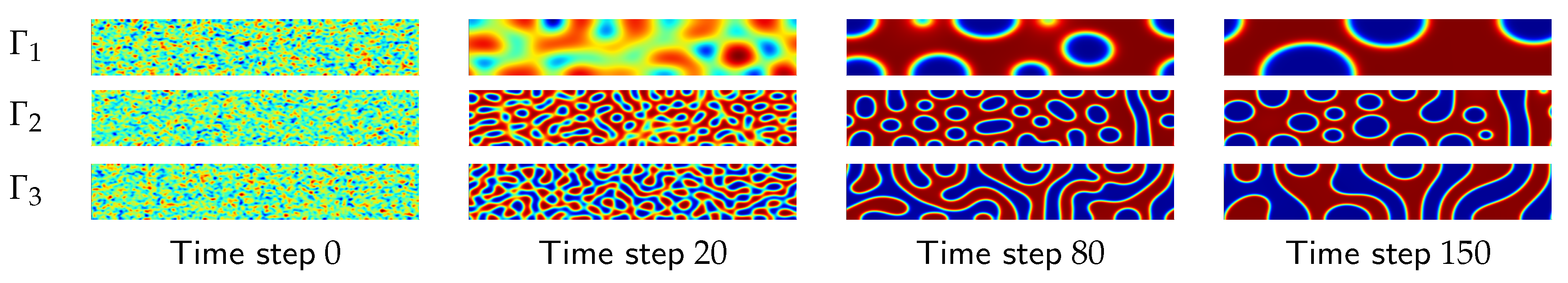
The key motivation behind this work arises from the massive and high-dimensional datasets that are produced by computational models that simulate material morphology evolution during the fabrication process of organic thin films (see Section 5.1), by solving nonlinear partial differential equations. Organic thin film fabrication is a key factor that controls the properties of organic electronics, such as transistors, batteries, and displays. However, this requires expensive search campaigns of the design space. Choice of the fabrication parameters impacts the trajectory that the process follows, which eventually determines the properties of the material being fabricated. Scientists and engineers are interested in using dimensionality reduction on the resulting big data to explore the material design space, and optimize the fabrication to make devices with desired properties.

In our prior work, we proposed S-Isomap, a spectral dimensionality reduction technique for nonlinear data [1] that can scale to massive data streams. While this method can efficiently and reliably process high-throughput data streams, it assumes that the input data are weakly correlated. Consequently, it fails when applied directly to process data. S-Isomap was derived from the standard Isomap algorithm [2], which is frequently used and favored in scientific computing data analysis [3,4,5,6,7,8]. Unfortunately, while there is some prior work on applying Isomap to spatio-temporal data [9], the focus has been on segmentation of data trajectories rather than discovering a continuous latent state. In our recent work, we proposed a new spectral method to handle high-dimensional process data [10].

This paper significantly expands on our past work [10] and makes two key contributions. The first contribution is to show how the standard linear and nonlinear dimensionality reduction methods, e.g., PCA, Isomap, etc., fail when dealing with process data. The poor performance can be attributed to the fact that every observation is highly correlated with the temporally close observations belonging to the same trajectory, and there is a lack of mixing (or cross-talk) between different trajectories of a process. The second contribution of this paper is a new method, Entropy-Isomap, which induces the cross-talk between different trajectories by adaptively modifying the neighborhood size for every data instance. The proposed method is both easy to implement and effective, and could likely be applied to other spectral dimensionality reduction methods, besides Isomap.

2. Background and Related Work

In this section we provide a gentle introduction to the spectral dimensionality reduction methods and the process data encountered in our target application, and also discuss some related techniques discussed in the literature for these topics.

2.1. Spectral Dimensionality Reduction Methods

Spectral dimensionality reduction (SDR) refers to a family of methods that map high-dimensional data to a low-dimensional representation by learning the low-dimensional structure in the original data. SDR methods rely on the assumption that there exists a function $f:{\mathbb{R}}^d\to {\mathbb{R}}^D$, $d\le D$, that maps low-dimensional coordinates, $y_i\in {\mathbb{R}}^d$, of each data sample to the observed $x_i\in {\mathbb{R}}^D$. The goal then becomes to learn the inverse mapping, $f^{-1}$, that can be used to map high-dimensional $x_i$ to low-dimensional $y_i$. While different methods exist within this family, they all share a common computing pattern. For a given set of points, $\mathbf{X}$, in a high-dimensional space ${\mathbb{R}}^D$, SDR methods compute either top or bottom eigenvectors of a feature matrix, $\mathbf{F}$ derived from the $n\times D$ data matrix, $\mathbf{X}$, where n is the number of data instances. Here, the feature matrix, $\mathbf{F}$, captures the structure of the data through some selected property (e.g., pairwise distances).

Two broad categories of SDR methods exist, based on the assumption they make about f (i.e., linear vs. nonlinear). Linear methods assume that the data lie on a low-dimensional subspace ${\mathbb{V}}^d$ of ${\mathbb{R}}^D$, and construct a set of basis vectors representing the mapping. When working with the linearity assumption, the most commonly used methods are PCA and multidimensional scaling (MDS) [11]. PCA learns the subspace that best preserves covariance, i.e., F is the $D\times D$ sample covariance matrix of the input data. The basis vectors learned by PCA, known as principal components, are the directions along which the data has highest variance. In the case of MDS, the feature matrix is the $n\times n$ dissimilarity matrix that encodes some pairwise relationships between data points in $\mathbf{X}$. When these relationships are Euclidean distances, the result is equivalent to that of PCA, and this is known as classical MDS. Spectral decomposition of F in both methods yields eigenvectors Q. Taking the top d eigenvectors, the data can be mapped to low-dimensions as $\mathbf{Y}$ by the transformation Y = X${\mathbf{Q}}_d$.

However, in cases where the data is assumed to be generated by some nonlinear process, the linearity assumption is too restrictive. In such cases, both PCA and MDS are not robust enough to learn the inverse mapping $f^{-1}$. Although variants of PCA have been proposed to address such situations (e.g., kernel PCA [12]), their performance is sensitive to the choice of the kernel and the associated parameters. Instead, the most common approach is to use a manifold learning-based nonlinear SDR (or NLSDR) technique, such as Isomap [2].

NLSDR techniques can be divided into two categories: global and local. Global methods, e.g., Isomap, minimum volume embedding [13], preserve a global property of the data. On the other hand, local methods, e.g., local linear embedding (LLE) [14,15], diffusion maps [16], Laplacian eigenmaps [17], preserve a local property for each data instance. All of these methods, however, involve a series of similar data transformations. First, a neighborhood graph is constructed, in which each node is linked with its k nearest neighbors. Next, this neighborhood graph is used to create a feature matrix which characterizes the property that the underlying algorithm is trying to preserve. For Isomap, the feature matrix is obtained as the shortest path graph in which every pair of data instances is connected to each other by the shortest path between them. The low-dimensional representation of the input data is obtained by factorization of the feature matrix. Typically, first d eigenvectors/values form the output Y. The steps of the Isomap algorithm are outlined in Algorithm 1.

Algorithm 1 ISOMAP

Input:$\mathbf{X}$, k

Output:$\mathbf{Y}$

1: ${\mathbf{D}}_{n\times n}$← PairwiseDistances($\mathbf{X}$) 2: ${\mathbf{G}}_{n\times n}$$\leftarrow \infty$ 3: for$x_i\in \mathbf{X}$do 4:  kNN← KNN($x_i$, $\mathbf{X}$, k) 5:  for $x_j\in$kNN do 6:   ${\mathbf{G}}_{i,j}\leftarrow {\mathbf{D}}_{i,j}$ 7: ${\mathbf{F}}_{n\times n}\leftarrow$ AllPairsShortestPaths($\mathbf{G}$) 8: $\mathbf{Y}\leftarrow \mathrm{MDS}\left(\mathbf{F}\right)$ 9: return$\mathbf{Y}$

2.2. Dynamic Process Data

If the rows in the input data matrix, $\mathbf{X}$, are uniformly sampled from the underlying manifold, methods such as Isomap are generally able to learn the manifold, in the presence of sufficient data. However, here, we consider the scenario where $\mathbf{X}$ represents a dynamic process, i.e., instances in $\mathbf{X}$ are partitioned into T trajectories, ${\Gamma }_1,{\Gamma }_2,\dots ,{\Gamma }_T$. ${\Gamma }_I$ represents one trajectory which is specified by a $\tau$-parameterized sequence of $m_I$ data points. Thus, the sum of the lengths of the T trajectories is equal to n, i.e., ${\sum }_T{m}_I=n$. In other words, ${\Gamma }_I$ = ($x_I\left({\tau }_1\right)$, $x_I\left({\tau }_2\right)$,…, $x_I\left({\tau }_{m_I}\right)$), where ${\tau }_i<{\tau }_j$ when $i<j$. Parameter $\tau$ usually denotes time, and trajectory ${\Gamma }_I$ can be a function of one or more additional parameters.

The target application for this study is the study of material morphology evolution during the fabrication of organic thin film [18]. In particular, we use process data produced by the numerical simulation of the morphology evolution. Each input trajectory (denoted as $\Gamma (\varphi ,\chi )$, from here on) corresponds to a simulation which is parameterized by two fabrication process variables, viz.: (i) $\varphi$, or the blend ratio of polymers making organic film; and (ii) $\chi$, or the strength of interaction between these polymers. Each trajectory consists of a series of “images”, generated over time, where each image is actually a 2D morphology snapshot that is produced by the numerical simulation for a given time step. A simple preprocessing step transforms the image to a high-dimensional vector, ${\mathbb{R}}^D$. See Figure 1 for some examples of the images that are generated for a selected combination of $\varphi$ and $\chi$. A detailed description of the data and the data generation process is provided in Section 5.

Ideally, to understand the impact of the input parameters, $\varphi$ and $\chi$, on the final properties of the material, a large number of simulations need to be run that can uniformly span the domains of $\varphi$ and $\chi$. However, the computational cost associated with generating one trajectory, corresponding to a single combination of $\varphi$ and $\chi$, means that the sampling is sparse. On the other hand, sampling in the time dimension is relatively dense. Instances belonging to the same trajectory tend to be strongly correlated, which is reflective of how the morphologies evolve. These factors strongly influence the connectivity of the neighborhood graph, G, which strongly impacts the approximation of the manifold distances by the Isomap algorithm.

2.3. Related Works in Dealing with Dynamic Processes

A significant body of work exists in the field of developing reduction strategies for high-dimensional data generated via complex physical processes. In fact, linear projection methods are often used to construct such reduced order models from high-dimensional data [19]. Nonlinear counterparts for such settings have been explored in limited settings, for certain types of dynamical systems [20,21,22,23]. In particular, several of these methods have adapted diffusion maps [16] to dynamical process data, by considering a fixed length “time-window” around each sample of the process data to define a local neighborhood, which can account for moderate noise at short temporal scales. However, most of these methods focus on understanding a single dynamical process, and not necessarily a collection of trajectories obtained by varying the parameter settings.

One recent work proposes a data-driven method for organizing temporal observations of dynamical systems that depend on the system parameters [24]. In that work, the authors simultaneously compute lower dimensional representations of the data along multiple dimensions, e.g., time, parameter space, initial variable space, etc. An iterative procedure is then applied, wherein every step involves mapping the data into a low-dimensional manifold using the diffusion maps algorithm for each dimension, then recomputing the distances between the observations (for each dimension) through a reconciliation step that utilizes information from other dimensions, and then repeating the process. While, one could adapt the above method for the problem discussed here, it is not designed to provide insights about the sparsely populated regions in the manifold, which is crucial to guide the next round of simulations in our target application.

3. Challenges of Using SDR with Dynamic Process Data

As mentioned earlier, PCA and Isomap are two standard off-the-shelf approaches to perform dimensionality reduction on high-dimensional data. However, if the method is applied without taking into consideration the underlying assumption of data linearity and uncorrelated samples, it delivers highly misleading results. Here, we study the effectiveness of both PCA and Isomap when dealing with dynamic process data.

3.1. Comparing PCA and Isomap for Dynamic Process Data

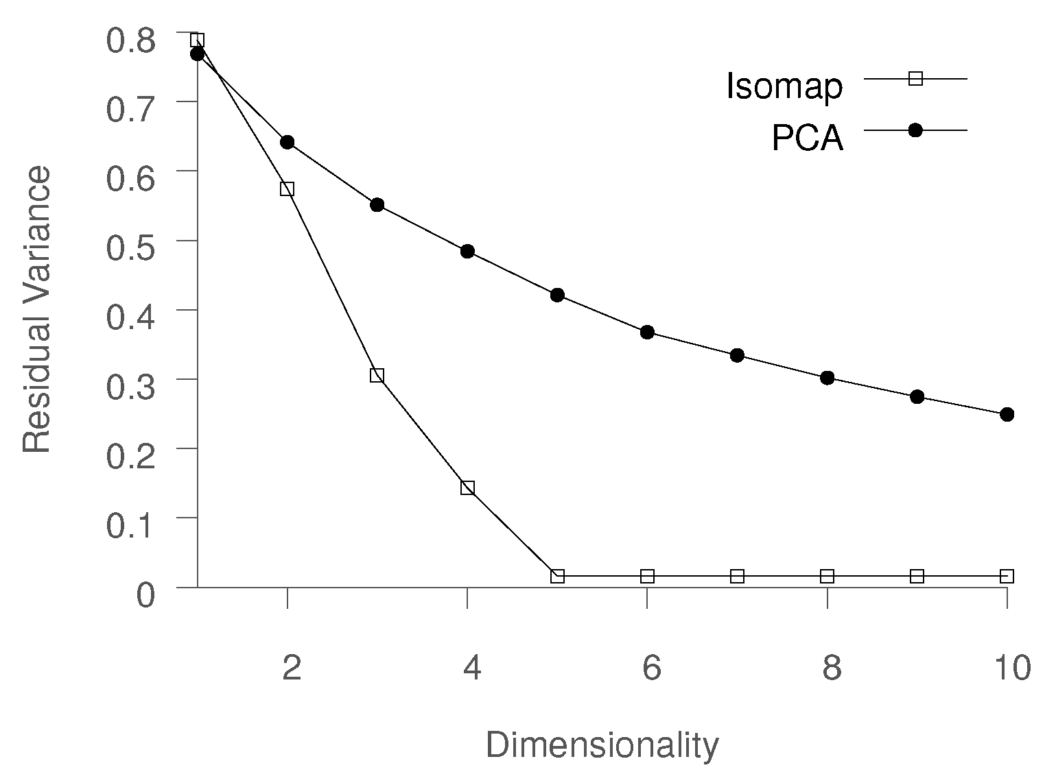
A reliable way of determining the quality of the low-dimensional representation (mapping) produced by each method is to compare the original data $\mathbf{X}$ in ${\mathbb{R}}^D$ with the mapped data $\mathbf{Y}$ in ${\mathbb{R}}^d$, by computing the residual variance. The process of computing residual variance for PCA differs from Isomap, but the values are directly comparable.

In PCA, each principal component (PC) explains a fraction of the total variance in the dataset. If we consider ${\lambda }_i$ as the eigenvalue corresponding to the ith PC and $|\Lambda |$ as the total energy in the spectrum, i.e., $|\Lambda |={\sum }_{i=1}^D{\lambda }_i$, then the variance explained by the ith PC can be computed as $\frac{{\lambda }_i}{|\Lambda |}$. The residual variance can be calculated as

$$R=1-\sum _{i=1}^d\frac{{\lambda }_i}{|\Lambda |}.$$

(1)

In the Isomap setting, residual variance is computed by comparing the approximate pairwise geodesic distances, computed in G represented by matrix ${\mathbf{D}}_G$ (recall that G is a neighborhood graph), to the pairwise distances of the mapped data $\mathbf{Y}$, represented by matrix ${\mathbf{D}}_Y$:

$$R=1-\rho {({\mathbf{D}}_G,{\mathbf{D}}_Y)}^2.$$

(2)

Here, $\rho$ is the standard linear correlation coefficient, taken over all entries of ${\mathbf{D}}_G$ and ${\mathbf{D}}_Y$.

To compare PCA and Isomap, we compare the residual variance obtained using PCA and Isomap on the earlier described material morphology evolution process data. The dataset consisted of six trajectories, corresponding to a unique combination of the parameters $\varphi$ and $\chi$. The comparison is shown in Figure 2. It is evident that PCA is not able to learn a reasonable low-dimensional mapping even when using 10 eigenvectors, while Isomap produces a highly accurate representation. For instance, while Isomap is able to explain about 70% of the variance using three dimensions, PCA requires more than nine dimensions. It should be noted that the ability to represent data in two or three dimensions is especially desired by domain experts, as it allows for data visualization and exploratory analysis.

If we visualize the data in 3D space using the PCA representation ($d=3$) (see Figure 3a), we observe that while PCA is able to describe the time aspect of the process evolution, it does not offer any additional insights into the process, making it ineffective for the task at hand. This can be primarily attributed to PCA’s inability to capture the nonlinear relationships between the high- and low-dimensional data.

The 3D visualization of Isomap is shown in Figure 3b. We note that despite the fact that Isomap is better than PCA at minimizing the residual variance, the low-dimensional trajectories do not offer meaningful insights. The trajectories appear to diverge from one another, leaving no reasonable interpretation of the empty space, whereas one would expect some ordering with respect to the $\varphi$ parameter. This indicates that the standard application of Isomap is inadequate when working with parameterized high-dimensional time series data. We obtain equally unsatisfactory results with other methods, including t-SNE and LLE [14,25].

3.2. Standard Isomap and Dynamic Process Data

While the Isomap trajectories in Figure 3b diverge from the initial time point, close inspection reveals that the trajectories exhibit nondivergent behavior in the earlier steps, which is expected since the morphologies are expected to evolve in a similar fashion at the beginning of the simulation.

We only applied Isomap to the early stage data represented by the first 30 time steps of each trajectory (the threshold was selected by the domain expert). The results are shown in Figure 3c. The results here are more encouraging as one can clearly observe that data points for all trajectories cluster together before quickly diverging. This observation points us to the key deficiency of Isomap when dealing with dynamic process data. When data instances exhibit strong temporal correlations, the neighborhood computation for any data instance in Isomap is heavily dominated by other instances belonging to the same trajectory. Thus, Isomap cannot capture the relationships across different trajectories and the reduced representation is dominated by the time dimension, as can be seen in Figure 3b.

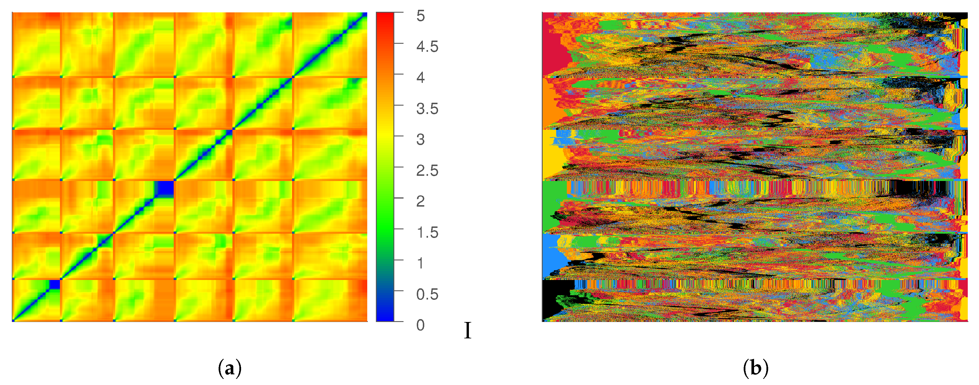
To further study this point, we consider the pairwise distance matrix $\mathbf{D}$ that contains the distance between every pair of data instances. The rows and columns of the matrix are ordered by the trajectory index and time, as shown in Figure 4a. Consider any pair of row (and column) indices, i and j, such that the trajectory index that contains the ith data instance is I, and the trajectory index that contains the jth data instance is J and ${\tau }_i$, and ${\tau }_j$ denotes the time index for each instance within the corresponding trajectory. Then, row i precedes row j in the matrix $\mathbf{D}$ if either $I<J$ or ${\tau }_i\le {\tau }_j$ if $I=J$.

We consider another visualization of this matrix (See Figure 4b), where the row ordering is retained, but each row contains the sorted distances (increasing order) of the corresponding data instance and all other instances in the dataset. We can observe that for the majority of instances, the first several nearest neighbors are always from the same trajectory. This is problematic because the ability of Isomap to learn an accurate description of the underlying manifold depends on how well the neighborhood matrix captures the relationship across the trajectories. We refer to this relationship as cross-talk, or mixing among the trajectories. For any given point, the desired effect would be that the nearest neighborhood set contains points from multiple trajectories. However, the sorted neighborhood matrix indicates a lack of mixing, which essentially means that the Isomap algorithm does not consider information from other trajectories when learning the shape of the manifold in the neighborhood of one trajectory.

3.3. Quantifying Trajectory Mixing

We propose a quantitative measure of the quality of neighborhoods in terms of the trajectory mixing by employing the information-theoretic notion of entropy. Consider any data instance, x, which belongs to trajectory ${\Gamma }_i$. Let $p_j$ be the fraction of k nearest neighbors of x that lie on a trajectory ${\Gamma }_j$. The entropy of the k-neighborhood of the data instance x is calculated as

$$H_x^k=\sum _{\forall j,p_j\ne 0}-p_j{log}_2{p}_j.$$

(3)

Similarly, we can define the k-neighborhood entropy for a trajectory ${\Gamma }_i$ as the average of k-neighborhood entropy for all data instances on the ith trajectory, i.e.,

$$H_{{\Gamma }_i}^k=\frac{1}{m_i}\sum _{x\in {\Gamma }_i}{H}_x^k.$$

(4)

Neighborhood entropy is directly related to the mixing of the trajectories in the proximity of a given data instance. If the neighborhood entropy of an instance is high, it means that the nearest neighbors of that instance exist in a large number of trajectories, indicating a strong mixing of the trajectories. On the other hand, if the entropy of a data instance is low, it means that the nearest neighbors lies on a single or very few trajectories, indicating a low level of mixing.

3.4. Strategies for Inducing Trajectory Mixing

One simple way to induce more trajectory mixing is to increase k, since this would increase the neighborhood entropy of the points. In considering the average neighborhood entropy for six individual trajectories for various values of k, we find that the neighborhood entropy increases linearly with k. Thus, for a small value of k, Isomap is unable to obtain a meaningful low-dimensional representation, as evident when using standard Isomap, as discussed above, where k was set to 8. In contrast, using large k could result in the desired level of trajectory mixing. However, as discussed in the Isomap paper [2], the approximation error between the true geodesic distance on the manifold between a pair of points and the approximate distance calculated using Dijkstra’s algorithm is inversely related to k. For large k, Isomap is essentially reduced to PCA, and is unable to capture the nonlinearities in the underlying manifold.

Another strategy to induce trajectory mixing is subsampling, i.e., selecting a subset of points from a given trajectory. However, this would result in reduction of the data, which yields poor results. Alternatively, we could use skipping in the neighborhood selection, i.e., for a given point, skip the s nearest points before including points in the neighborhood. Unfortunately, in experimenting with skipping and subsampling approaches we experienced a loss in local manifold quality or data size, respectively. On the basis of this and the desire to achieve the most accurate local and global qualities, we propose an entropy-driven approach in the next section.

4. Entropy-Isomap

As we established earlier, standard Isomap does not work well for dynamic process data since neighboring data points are typically from the same trajectory. However, the global structure of the process manifold is determined by the relations between different trajectories. When k-NN neighborhoods are computed, this can result in poor mixing of the trajectories. The mixing can also vary depending on the temporal location of the process. For example, if the trajectories are generated using similar initial conditions, the trajectories will exhibit strong mixing. However, the trajectories typically diverge subsequently. A neighborhood size k that produces good results in early stages might produce poor results later on in the process. A value of k that is large enough to work for all times might include so many data points that the geodesic and Euclidean distances become essentially the same, which results in a PCA-like behavior, defeating the purpose of using Isomap.

To address this situation, we propose to directly measure the amount of mixing and use it to change the neighborhood size for different data points adaptively. This mitigates the shortcomings of the two methods described in the previous section, which either discard data (subsampling) or lose local information (skipping).

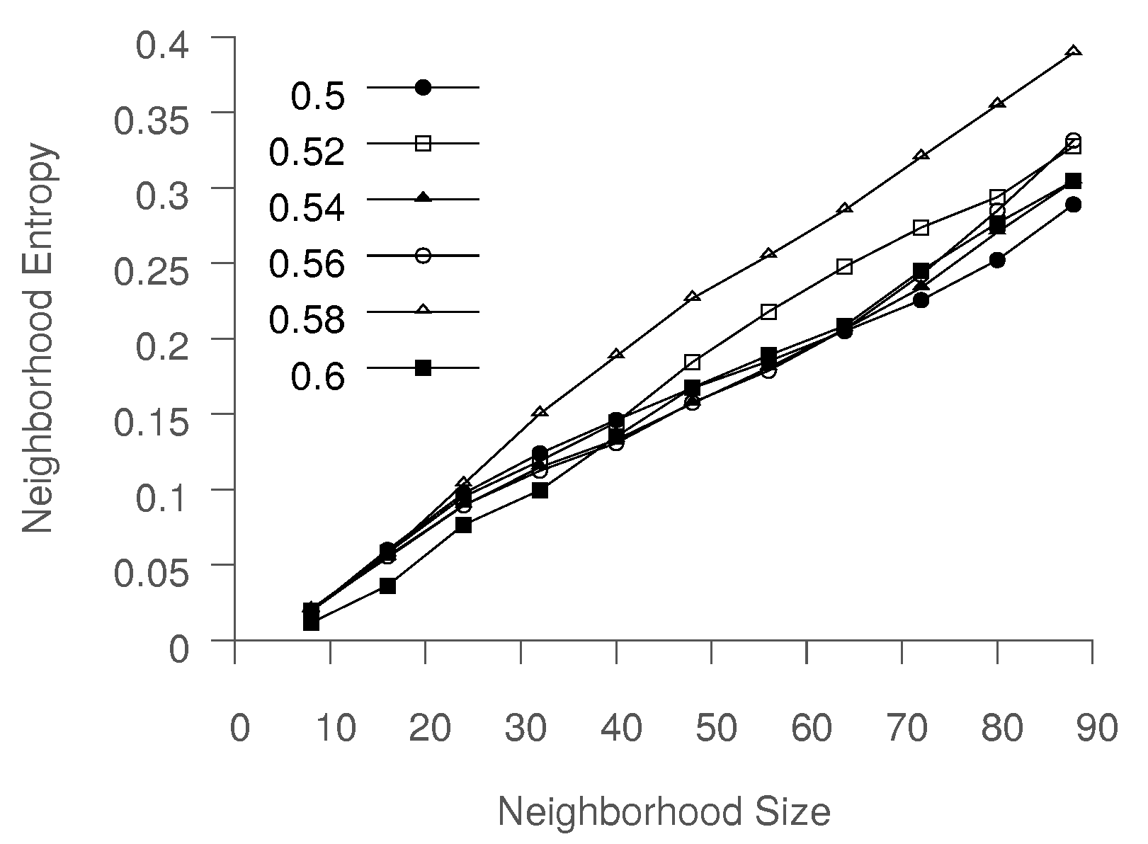
Figure 5 shows that neighborhood entropy increases when the next nearest neighbors are added. We propose using a threshold on the neighborhood entropy, as defined above, to adaptively determine an appropriate neighborhood size, k. This modification allows the flexibility of larger neighborhoods in regions where it is necessary or desired to force mixing between trajectories.

An additional parameter, M, determines the largest possible neighborhood size. This user-defined parameter is used to ensure that the neighborhoods are not so large as to reduce Isomap to PCA. For datasets which contain trajectories in poorly sampled regions of the state space, M controls the size of the local neighborhood, without skewing the rest of the analysis, which would otherwise result in an unreasonably large value of k.

Algorithm 2 outlines the step of the proposed Entropy-Isomap algorithm. While the proposed algorithm has some similarities to the standard Isomap algorithm (See Algorithm 1), there are some key differences. First, the algorithm takes two additional arguments, the target entropy level, $\widehat{H}$ to determine the optimal neighborhood size, and the maximum neighborhood size, M. The initial step, computing all pairwise distances for data instances in $\mathbf{X}$, remains the same as in the standard algorithm. Next, the algorithm performs the entropy-based neighborhood selection (lines 3–9). For each point $x_i$, the algorithm starts with an initial neighborhood size, k, and identifies the k-nearest neighbors. These are used to compute the neighborhood entropy for the data instance. If the entropy threshold $\widehat{H}$ is not satisfied, then $k_i$ is incremented (line 6), and the process repeats. Once the entropy threshold is reached, or if $k_i$ reaches the maximum threshold of M, the process terminates. The entire process is repeated for each $x_i$, and after all neighborhoods have been identified, the algorithm continues the same way as standard Isomap (lines 10–12). While this iterative strategy for identifying optimal neighborhood size for each data instance appears to be inefficient, it is presented here for more clarity. In practice, the optimal neighborhood determination can be made via a more efficient binary search-based strategy.

Algorithm 2 ENTROPY-ISOMAP

Input:$\mathbf{X}$, k, $\widehat{H}$, M

Output:$\mathbf{Y}$

1: ${\mathbf{D}}_{n\times n}$← PairwiseDistances(X) 2: ${\mathbf{G}}_{n\times n}$$\leftarrow \infty$ 3: for all$x_i\in \mathbf{X}$do 4:  $k_i\leftarrow k$ 5:  while $H<\widehat{H}$ and $k_i<(M+k)$ do 6:   $k_i\leftarrow k_i+1$ 7:   kNN← KNN($x_i$, $\mathbf{X}$, $k_i$) 8:   ${\mathbf{G}}_{i,j}\leftarrow {\mathbf{D}}_{i,j}$ where $x_j\in$ kNN. 9:   $H\leftarrow$ NeighborhoodEntropy(x, $k_i$, $\overline{G_i}$) 10: ${\mathbf{F}}_{n\times n}\leftarrow$ AllPairsShortestPaths($\mathbf{G}$) 11: $\mathbf{Y}\leftarrow \mathrm{MDS}\left(\mathbf{F}\right)$ 12: return$\mathbf{Y}$

We applied Entropy-Isomap to the process data discussed earlier, with $k=8$ and the maximum number of steps $M=100$. The large M ensures that the algorithm is able to create very large neighborhoods to strictly enforce trajectory mixing. To understand the behavior of the method as a function of the entropy threshold, $\widehat{H}$, we varied $\widehat{H}$ from $0.1$ to $0.9$. The example low-dimensional representation obtained by Entropy-Isomap is presented in Figure 6b.

Figure 7b shows how the final neighborhood entropy for the instances belonging to six trajectories vary according to time. We note that, for this data, the threshold for entropy ($\widehat{H}$, set to 0.3 for this experiment) is often not reached even after expanding $k_i$. Instead, the neighborhood size reaches the maximum limit, M. We believe that this is because the k nearest neighbors for the majority of points are in the same trajectory, (see Figure 4b), which leads to skewed neighborhood distributions. As a result, even when a satisfactory number of neighbors come from other trajectories, the entropy for the neighborhood might be low. Even when the trajectories mix, the neighborhoods are still dominated by other instances in the same trajectory, as shown in Figure 6c. Therefore, while high entropy implies good mixing, the converse is not necessarily true. Large neighborhoods could produce mixing, while still having low entropy. Thus, the entropy threshold is set to be around 0.30–0.40, with further confirmation through experimentation being presented in the next section.

If the entropy threshold is strictly enforced, one will have to increase the neighborhood size. For the process data, we observed that the neighborhood sizes will become very large. Figure 7a shows the neighborhood size distribution for $\widehat{H}=0.30$. For such values of k, the method simply reduces to PCA, a linear method, which suffers from limited expressiveness because of the linearity assumption.

Points that produce no mixing also end up with large neighborhoods, as Entropy-Isomap tries to increase $k_i$ in order to meet the entropy threshold. These points occur when the dataset does not contain enough trajectories that pass near those particular states to produce good geodesic distance estimates. Interestingly, we found that plotting entropy versus time in Figure 7b reveals that trajectories can pass through poorly sampled parts of the state space and again “meet up” with other trajectories.

The proposed methods can be used to detect trajectories that do not interact and also which regions of the state space are poorly sampled. This can be used to either remove them from the dataset or as a guide to decide where to collect more process data.

5. Application

The current work is motivated by the need to analyze and understand big datasets arising in the manufacturing of organic electronics (OEs). OE is a new sustainable class of device, spanning organic transistors [26,27], organic solar cells [28,29], diode lighting [30,31], flexible displays [32], integrated smart systems such as RFIDs (Radio-frequency Identification) [33,34], smart textiles [35], artificial skin [36], and implantable medical devices and sensors [37,38]. The critical and highly desirable features of OEs are their cost, and their rapid and low-temperature roll-to-roll fabrication. However, many promising OE technologies are bottlenecked at the manufacturing stage, or more precisely, at the stage of efficiently choosing fabrication pathways that would lead to the desired material morphologies, and hence device properties.

The final properties of OEs (e.g., electrical conductivity) are a function of more than a dozen material and process variables that can be tuned (e.g., through evaporation rate, blend ratio of polymers, final film thickness, solubility, degree of polymerization, atmosphere, shearing stress, chemical strength, and frequency of patterning substrate), leading to the combinatorial explosion of manufacturing variants. Because the standard trial-and-error approach, in which many prototypes are manufactured and tested, is too slow and cost inefficient, scientists are investigating in silico approaches [39,40]. The idea is to describe the key physical processes via a set of differential equations, and then perform high-fidelity numerical simulations to capture the process dynamics in relation to input variables. Then, the problem becomes to identify and simulate some initial set of manufacturing variants, and use analytics of the resulting process data to first understand the process dynamics (e.g., rate of change in domain size or the transition between different morphological classes), and then identify new promising manufacturing variants.

The key scientific breakthroughs that improved organic solar cell (OSC) performance were closely related to the manufacturing pathway. Most advances have been achieved by nontrivial and nonintuitive (and sometimes very minor) changes in the fabrication protocol. Classic examples include changing the solvent [41], and thermal annealing [42], which together resulted in a two orders of magnitude increase in the efficiency of OSCs. These advances have reaffirmed the importance of exploring processing conditions to impact device properties, and have resulted in the proliferation of manufacturing variants. However, these variants are invariably chosen using trial-and-error approaches, which has resulted in the exploration of very scattered and narrow zones of the space of potential processing pathways due to resource and time constraints.

5.1. Data Generation

The material morphology data analyzed in this paper was generated by a computational model based on the phase-field method of recording the morphology evolution during thermal annealing of the organic thin films [18,43]. We focused on the exploration of two manufacturing parameters: blend ratio $\varphi$ and strength of interaction $\chi$. We selected these two parameters, since they are known to strongly influence the properties of the resulting morphologies. For each fabrication variant ($\varphi ,\chi$), we generated a series of morphologies that together formed one trajectory $\Gamma (\varphi ,\chi )$.

We selected the range of our design parameters $\varphi =[0.5,0.6]$ and $\chi =[2.2,3.0]$ to explore several factors. First, we were interested in two stages of the process: early materials phase separation and coarsening. Moreover, we wanted to explore various topological classes of morphologies. In particular, we were interested in identifying the fabrication conditions leading to interpenetrated structures. Finally, we hoped to find the optimal annealing time that results in desired material domain sizes. In total, we generated 16 trajectories, with, on average, 180 morphologies per trajectory. Each morphology was represented as an image converted into a $40,000$ dimensional space defined by pixel composition values. The entire data used in our experiments as well as the source code of the method are open and available from https://gitlab.com/SCoRe-Group/Entropy-Isomap.

5.2. Results

For the target application of optimal manufacturing design, we leveraged dimensionality reduction to gain insights into the morphological data. First, we aimed to discover the latent variables governing the associated dynamic process. Second, we aimed to unravel the topology of the manifold in order to explore the input parameter space and ultimately identify the manufacturing variant that leads to the desired morphology.

Using Entropy-Isomap, we performed the analysis for a set of morphological pathways. In Figure 8 and Figure 9, we depict the discovered three-dimensional manifold for the set of 16 pathways. In the discovered manifold, the individual pathways are ordered according to process variables that were varied to generate the data. In each figure, the same manifold is depicted eight times. For easier inspection, each variant is individually color coded. The panels in the top row of Figure 8 depict the pathways for fixed $\varphi$ and varying $\chi$. We observe that the pathways for increasing $\varphi$ are ordered from front to back. The panels in the bottom row of Figure 8 highlight the pathways for increasing $\chi$. Similarly to the top row, we observe the pathways to be ordered from right to left.

Figure 8 depicts the manifold for the early stages of morphology evolution, while Figure 9 depicts the manifold for a longer evolution time. However, in both cases, the observed ordering is consistent. The pathways for increasing $\chi$ are ordered from the right (dark) to the left (light), while the pathways for increasing $\varphi$ are ordered from the front (green) to back (blue).

The observed ordering of pathways strongly indicates that the input variables are also the latent variables controlling the dynamics of the process. The discovered manifold also reveals that denser sampling is required along the blend ratio space variable ($\varphi$). Specifically, the pathways sharing the same $\chi$ but varying $\varphi$ are spread further apart on the manifold than those sharing the same $\chi$ value. This observation has important implications for the exploration of the design space. In particular, adding more sampling points in the $\varphi$ space offers higher exploration benefits, while adding more points in the $\chi$ space improves exploitation chance. This indicates that the $\varphi$ space should be explored first, followed by a potential exploitation phase.

Finally, using Entropy-Isomap, we identified two regimes in the manifold. Morphologies in the early stages of the process are mapped to evolve in the radial direction, while morphologies in late stages are mapped to evolve parallel to each other. This is interesting as the underlying process indeed has two inherent time scales. In the early stage, the fast and dynamic phase separation between the two polymers occurs. During this stage, the composition of the individual phases changes significantly. These changes mostly increase composition amplitude. In the second stage, the equilibrium composition is already established. The coarsening between already formed domains dominates the dynamics of the process. Here, the amplitude of the composition (signal) does not change significantly. The changes mostly occur in the frequency space of the domain size, with the domain sizes increasing over time.

6. Conclusions and Future Directions

Existing spectral dimensionality reduction methods do not work well when the underlying data exhibits a temporal correlation, as is the case with dynamic process data. We propose using the notion of neighborhood entropy to quantitatively determine the amount of information exchanged among data instances, independent of the temporal component. On the basis of this measure, we propose the Entropy-Isomap algorithm, which uses the entropy of the neighborhood to adaptively increase the neighborhood size, and thus facilitate cross-talk across different process trajectories.

We show how the proposed methodology can be used to better understand the morphology evolution of two immiscible materials. In future, the proposed approach can be leveraged for the smart and autonomous exploration of the manufacturing design spaces in organic electronics. The notion of mixing between individual trajectories can be used to detect the underexplored parts in the design, thus helping to build more reliable manifolds and increase confidence in the understanding of the dynamic process. The reduced order representation learnt by the proposed method shows a clear ordering of the trajectories according to the process variables. At the same time, the learnt representation reveals sparsely populated regions in the manifold, motivating the need for more samples in those regions. Thus, this insight can provide guidance in terms of designing the next round of simulations that can generate data corresponding to the undersampled process configurations. More importantly, the exposed undersampled regions of the design space can be used for active learning of the dynamic processes, potentially reducing the number of required numerical experiments to discover a stable manifold. Another promising direction is the use if a Bayesian surrogate, e.g., a Gaussian process-based model [44], as well as the use of predictive variance to execute the smart exploration of the manufacturing process.