Article

Kernel Identification of Non-Linear Systems with General Structure

Faculty of Electronics, Wrocław University of Science and Technology, 50-372 Wrocław, Poland
*
Author to whom correspondence should be addressed.
Algorithms 2020, 13(12), 328; https://doi.org/10.3390/a13120328
Submission received: 27 October 2020 / Revised: 3 December 2020 / Accepted: 4 December 2020 / Published: 6 December 2020

Abstract

:
In the paper we deal with the problem of non-linear dynamic system identification in the presence of random noise. The class of considered systems is relatively general, in the sense that it is not limited to block-oriented structures such as Hammerstein or Wiener models. It is shown that the proposed algorithm can be generalized for two-stage strategy. In step 1 (non-parametric) the system is approximated by multi-dimensional regression functions for a given set of excitations, treated as representative set of points in multi-dimensional space. ‘Curse of dimensionality problem’ is solved by using specific (quantized or periodic) input sequences. Next, in step 2, non-parametric estimates can be plugged into least squares criterion and support model selection and estimation of system parameters. The proposed strategy allows decomposition of the identification problem, which can be of crucial meaning from the numerical point of view. The “estimation points” in step 1 are selected to ensure good task conditioning in step 2. Moreover, non-parametric procedure plays the role of data compression. We discuss the problem of selection of the scale of non-parametric model, and analyze asymptotic properties of the method. Also, the results of simple simulation are presented, to illustrate functioning of the method. Finally, the proposed method is successfully applied in Differential Scanning Calorimeter (DSC) to analyze aging processes in chalcogenide glasses.

1. Introduction

The problem of non-linear system modeling has been intensively examined over the past four decades. Owing to many potential applications (see [1]) and interdisciplinary scope of the topic, both scientists and engineers look for more precise and numerically efficient identification algorithms. First attempts at generalization of linear system identification theory for non-linear models were based on Volterra series representation ([2]). Traditional Volterra series-based approach leads to relatively high numerical complexity, which is often not acceptable from practical point of view. To cope with this problem regularization or tensor network techniques have been proposed recently ([3,4]). However, strong restrictions are imposed on the system characteristics (e.g., smoothness of nonlinearity, and short memory of the dynamics). Alternatively, the concept of block-oriented models was introduced ([5]). It was assumed that the system can be represented, or approximated with satisfactory accuracy, with the use of structural models including interconnected elementary blocks of two types—linear dynamics and static nonlinearities ([6]). The most popular structures in this class are Hammerstein system (see e.g., [7,8,9,10,11,12]) with static nonlinearity followed by linear dynamics, and the Wiener system [13,14,15,16,17,18]) including the same blocks connected reversely.
Traditionally, identification method needs two kinds of knowledge—set of input–output measurements and a priori parametric formula describing system characteristics and including finite number of unknown parameters ([6,19]). Usually, the polynomial model of static characteristics and the difference equation with known orders are assumed. This convention leads to relatively fast convergence of parameter estimates, but the risk of systematic approximation error appears, if the assumed model is not correct. As an alternative, the theory of non-parametric system identification ([20,21,22,23]) was proposed to solve this problem. The algorithms work under mild prior restrictions, such as stability of linear dynamic block and local continuity of static non-linear characteristics. Although the estimates converge to the true characteristics, the rate of convergence is relatively slow in practice, as a consequence of assumptions relaxation.
This paper represents the idea of combined, i.e., parametric-non-parametric, approach (see e.g., [24,25,26,27,28,29,30]), in which both parametric and non-parametric algorithms support each other to achieve the best possible results of identification for moderate number of measurements and to guarantee the asymptotic consistency (i.e., convergence to the true system characteristics), when the number of observations tends to infinity. Since the preliminary step of structure selection is treated rather cursorily in the literature, generalizations of the approach towards wider classes of systems seem to be of high importance from practical point of view. The paper was also motivated by the project of Differential Scanning Calorimeter ([31]) developed in the team, and particularly, modeling of heating process for examination the properties of chalcogenide glasses.
Main contribution of the paper lays in the following aspects:
  • proposed identification algorithm is run without any prior knowledge about the system structure and parametric representation of nonlinearity,
  • non-parametric multi-dimensional kernel regression estimate was generalized for modeling of non-linear dynamic systems, and the dimensionality problem was solved by using special input sequences,
  • the scheme elaborated in the paper was successfully applied in Differential Scanning Calorimeter for testing parameters of chalcogenide glasses.
The paper is organized as follows. In Section 2 the general class of considered systems and the identification problem is formulated in detail. Next, in Section 3.1, purely non-parametric, regression-based approach is presented, and its disadvantages are discussed. Then, to cope with dimensionality problem, the idea of some specific input sequences is presented in Section 3.2. Owing to that, the system characteristics are identified only for some selected points, but the convergence is much faster. The idea of combined, two-stage strategy is introduced in Section 4. It allows use of prior knowledge to expand the model on the whole input space. Also, the results of simple simulation are included in Section 5 to illustrate and discuss some practical aspects of the approach. Finally, in Section 6, the algorithm is successfully applied in Differential Scanning Calorimeter to model aging properties of modern materials (chalcogenide glasses).

2. Problem Statement

2.1. Class of Systems

We consider discrete-time non-linear dynamic system with general representation
y k = F u k i i = 0 + z k ,
where u k i i = 0 is bounded random input sequence ( u k < u max ), z k is zero mean random disturbance. The transformation F is Lipschitz with respect to all arguments, and has the property of exponential forgetting (fading memory), i.e., if we put u k i = 0 for i s and define the cut-off sequence as
u ¯ k i u k i , as i = 0 , 1 , . . . , s 1 0 , as i s ,
We assume that it holds that
Δ s F u k i i = 0 F u ¯ k i i = 0 c λ s ,
with some unknown c = const , and 0 < λ < 1 . Similar class of fading memory systems, in which the output depends less and less on historical inputs, was considered in [32]. The goal is to identify the system (build the model F ^ ) using the sequence of N input–output measurements u k , y k k = 1 N .
In considered system class, hysteresis is not admitted.

2.2. Examples

In this section, we show that some systems (popular in applications) fall into above description as special cases.

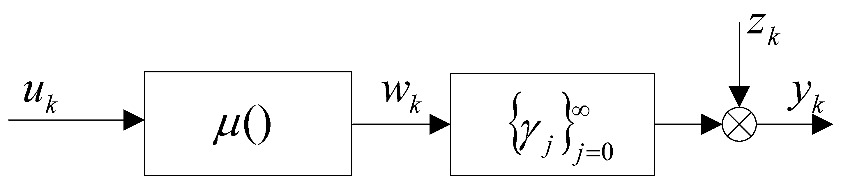
2.2.1. Hammerstein System

For Hammerstein system (see Figure 1), described by the equation
y k = i = 0 γ i μ u k i + z k
with the Lipschitz non-linear characteristic, i.e., such that
μ u a μ u b l u a u b ,
and asymptotically stable dynamics, i.e., γ i c H λ i , we get
Δ s = i = s γ i μ u k i μ 0 l u max i = s γ i c λ s .

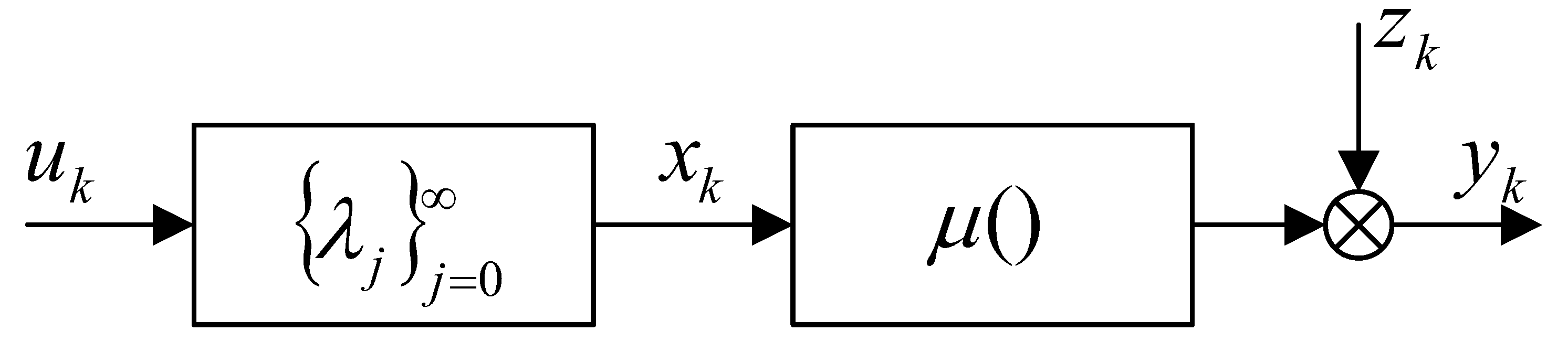
2.2.2. Wiener System

Analogously, for Wiener system (Figure 2), where the stable linear dynamics is followed by the Lipschitz static non-linear block
y k = μ i = 0 λ i u k i + z k ,
We get
Δ s = μ i = 0 γ i u k i μ i = 0 s 1 γ i u k i
l i = s γ i u k i < c λ s .
Remark 1.
Analogously, it can be simply shown that also Wiener–Hammerstein (L–N–L) and Hammerstein–Wiener (N–L–N) sandwich systems belong to the assumed class.

2.2.3. Finite Memory Bilinear System

Another important and often met in application special case is the bilinear system with finite order m. It is described by the formula
y k = l 0 , l 1 , . . . , l m 1 : l i 0 i l i m c l 0 , l 1 , . . . , l m 1 i = 0 m i u k i l i + z k
i.e., for m = 1 we get
y k = c 0 , 0 + c 1 , 0 u k + c 0 , 1 u k 1 ,
for m = 2 we have that
y k = c 0 , 0 + c 1 , 0 u k + c 0 , 1 u k 1 + c 1 , 1 u k u k 1 + c 2 , 0 u k 2 + c 0 , 2 u k 1 2 .
Since y k does not depend on u k m , u k m 1 , . . . , for s m we get F u k i i = 0 = F u ¯ k i i = 0 , and obviously Δ s = 0 .
Considered example falls into the more general class of Volterra representation. Presented approach works without the knowledge of parametric representation. As regards applicability to the class (1), for m < we have finite memory system, i.e., Δ ( s ) = 0 , as s > m . Moreover, since the input is assumed to be bounded ( u k < u max ), resulting mapping F ( ) fulfills Lipschitz condition (as ordinary polynomial on compact support).

3. Non-Parametric Regression

3.1. General Overview

Let us introduce the s-dimensional input regressor
u k ( s ) = u k , u k 1 , . . . , u k ( s 1 ) T ,
and the regression function
R s x ( s ) = E y k | u k ( s ) = x ( s ) ,
with the argument vector
x ( s ) = x 0 , x 1 , . . . , x s 1 T .
In particular, for s = 1 we get
R 1 x 0 = E y k | u k = x 0 ,
and for s = 2
R 2 ( x 0 , x 1 ) = E y k | u k = x 0 u k 1 = x 1 .
The non-parametric kernel estimate ([20,21,22,23,33]) of R s x ( s ) has the following form
R ^ s x ( s ) = k = 1 N y k K u k ( s ) x ( s ) h k = 1 N K u k ( s ) x ( s ) h ,
where · denotes Euclidean norm, K plays the role of kernel function, e.g.,
K v = 1 , as v 1 0 , as v > 1 ,
and h is a bandwidth parameter, responsible for the balance between bias and variance of the estimate. The class of possible kernels can obviously be generalized. Nevertheless, previous experiences shows that the kind of kernel function used for estimation is of secondary importance, whereas behavior of h ( N ) with respect to N is fundamental. We limited the presentation to Parzen (window) kernel for clarity of exposition. It fulfills all general assumptions made for kernels, i.e., it is even, non-negative and square integrable. The system (1) is thus approximated by the model
R ^ s u k , u k 1 , . . . , u k ( s 1 ) ,
and s can be interpreted as its complexity. Obviously, both h = h ( N ) and s = s ( N ) need to be set depending on the number of measurements N. Observing that
F u k i i = 0 = R u k ( ) ,
the mean squared error of the model R ^ s u k ( s ) can be expressed as follows
M S E R ^ s u k ( s ) = E R ^ s u k ( s ) F u k i i = 0 2 = E R ^ s u k ( s ) R u k ( ) 2 ,
and introducing the true finite-dimensional regression function R s u k ( s ) we get
M S E R ^ s u k ( s ) = E R ^ s u k ( s ) R s u k ( s ) + R s u k ( s ) R u k ( ) 2 = E R ^ s u k ( s ) R s u k ( s ) 2 + E R s u k ( s ) R u k ( ) 2 + + 2 E R ^ s u k ( s ) R s u k ( s ) R s u k ( s ) R u k ( ) .
Since both E R s u k ( s ) R u k ( ) 2 0 as N and R s u k ( s ) R u k ( ) 0 as N , these components can be set arbitrarily small by using appropriate scale s. Owing to above, for fixed s we focus on the first component of the MSE error of the form
E R R = E R ^ s u k ( s ) R s u k ( s ) 2 = b i a s 2 R ^ s u k ( s ) + v a r R ^ s u k ( s ) ,
where
b i a s R ^ s ( u k ( s ) ) E R ^ s ( u k ( s ) ) R s ( u k ( s ) ) ,
v a r R ^ s ( u k ( s ) ) E R ^ s ( u k ( s ) ) E R ^ s ( u k ( s ) ) 2 .
It can simply be shown that
b i a s R ^ s x ( s ) = o h ( N ) ,
b i a s 2 R ^ s x ( s ) = o h 2 ( N ) ,
The bias order follows directly from Lipschitz condition, and the fact that u k ( s ) x [ p ] ( s ) h for all k’s selected by kernel. Moreover,
v a r R ^ s x ( s ) = o 1 N h s N .
For window kernel, Lipschitz function F , and strictly positive input probability density function around the estimation point, probability of selection in s-dimensional space can be obviously evaluated from below by c h s , where c is some constant. Hence, expected number of successes is proportional to N c h s (not less than). The variance order is thus a simple consequence of Wald’s identity. Hence, to assure the convergence R ^ s x ( s ) R s x ( s ) , as N in the mean square sense, the following conditions must be fulfilled
h 0 and N h s , as N ,
which leads to typical setting
h ( N ) N α , where α 0 , 1 s .
To obtain the best asymptotic trade-off between squared bias and variance and comparing its orders we get
h 2 ( N ) = 1 N h s N ,
h s + 2 ( N ) = 1 N ,
h o p t N N 1 s + 2 ,
E R R N 2 s + 2 .
Moreover, to assure the balance between the estimation error and approximation error of order o ( λ s ) , connected with neglecting the tail u k i i = s we get
N 2 s ( N ) + 2 = λ s ( N ) ,
2 s ( N ) + 2 log N = s ( N ) log λ ,
2 s ( N ) s ( N ) + 2 = log λ log N ,
s 2 N + 2 s N = 2 log 1 λ log N ,
where 2 log 1 λ = const . Owing to above, the scale s N must not be faster than log N , i.e.,
s o p t ( N ) = O log N .
which illustrates slowness of admissible model complexity increasing in general case. The property (38) commonly known as “curse of dimensionality problem” illustrates the main drawback of multi-dimensional non-parametric regression approach to system modeling in traditional form. The reason is that probability of kernel selection
P K u k ( s ) x ( s ) h = 1 = P u k ( s ) x ( s ) h h s
decreases rapidly when s grows large. We also refer the reader to the proof of Theorem 3 in [26], where a detailed discussion concerning an analogous problem can be found.

3.2. Dimension Reduction

To cope with the problem shown in (39) we consider two cases of some specific input excitation processes to speed up the rate of convergence.

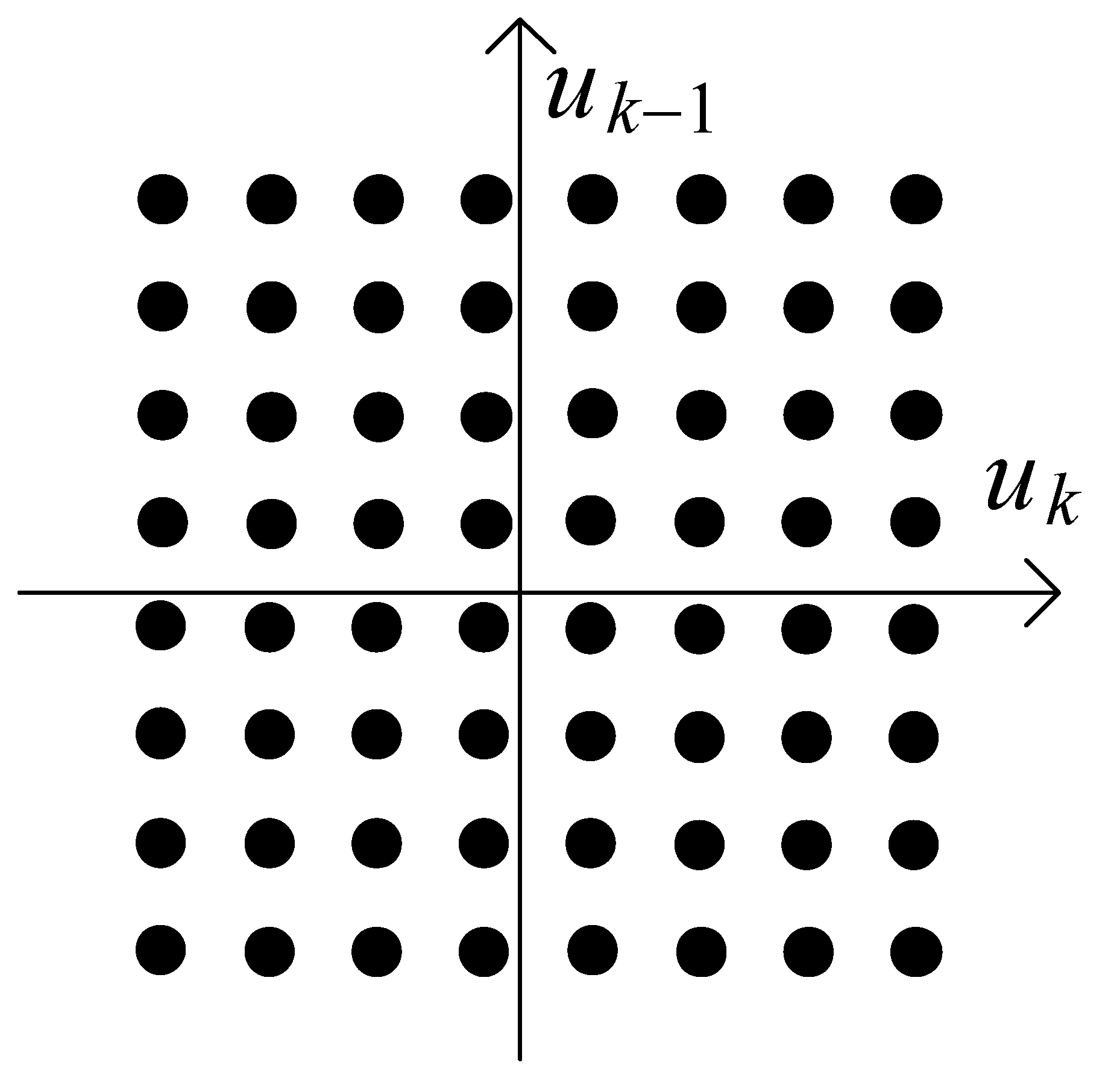
3.2.1. Discrete Input

In case 1 we assume that in each s-element input sub-sequence u k , u k + 1 , . . . , u k + s 1 , there exists d inputs with discrete distribution on finite set of possible realizations. Consequently, all the points u k ( s ) R s lay on a finite number of separable and compact subspaces with the internal dimension
s * = s d ,
and for x ( s ) = u k ( s ) we have
E R R N 2 s * + 2 .
For each measurement point probability of kernel selection behaves like c h s * , where s * , ( s * < s ) , is internal dimension of this subspace. In particular, for d = s (all input variables quantized) we get E R R N 1 . The sets of possible input sequences for s = 2 are illustrated in Figure 3 and Figure 4.

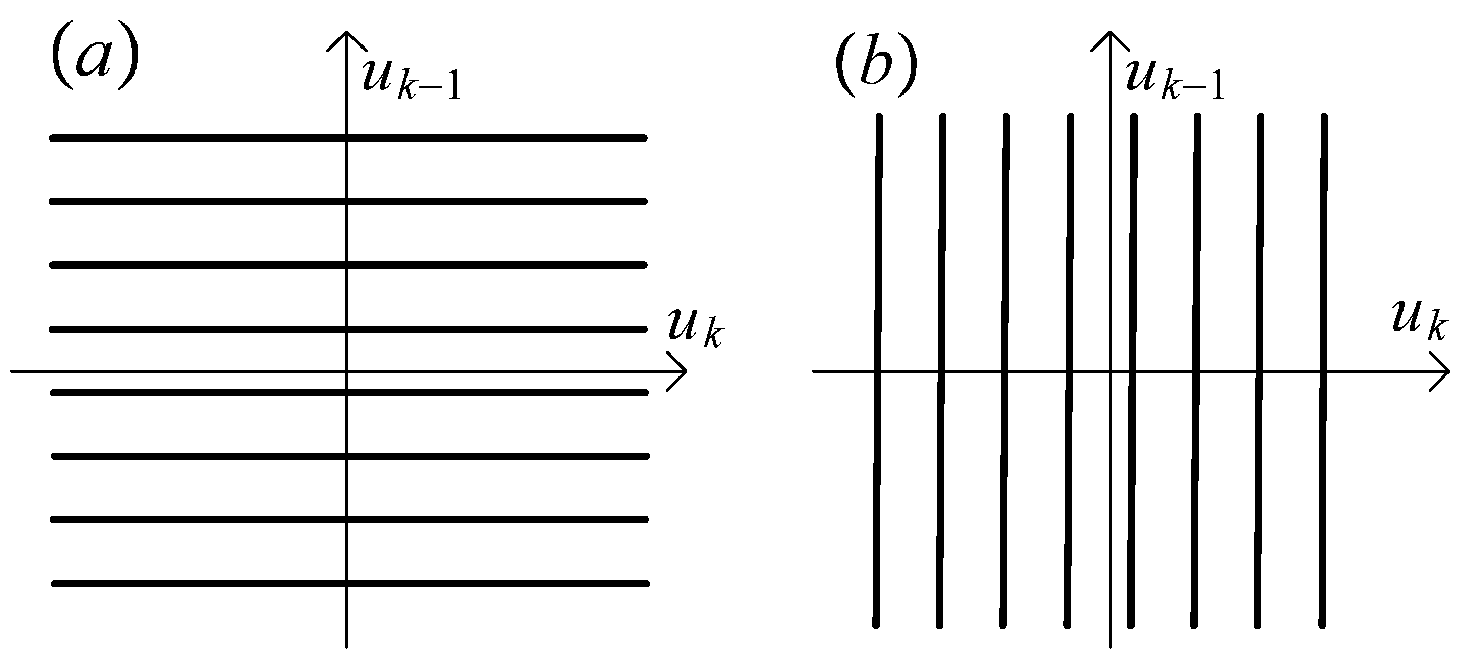
3.2.2. Periodic Input

In case 2 we assume the input is periodic with the period N 0 , i.e., u k = u k + N 0 for each k = 1 , 2 , . . . , N N 0 . Then, the value of the regressor u k ( s ) (see (13)) evaluates to one of N 0 distinct points in R s , n Z ,
x [ 1 ] ( s ) = u s u s 1 u 1 , . . . , x [ N 0 ] ( s ) = u N 0 + s 1 u N 0 + s 2 u N 0
with probabilities
P u k ( s ) = x [ p ] ( s ) = 1 N 0 , p = 1 , 2 , . . . , N 0
Measurements are uniformly distributed on the finite set of N 0 distinct points
x [ 1 ] ( s ) , . . . , x [ p ] ( s ) , . . . x [ N 0 ] ( s )
Narrowing of h ( N ) does not affect the kernel estimator asymptotically (i.e., s * = 0 ). Consequently, we get the best possible convergence rate E R R N 1 . However, it must be admitted that estimators are calculated only for finite number of points, and, increasing N 0 causes increase of variance of the regression estimator for particular points x [ p ] ( s ) (as the number of selected data is of order N / N 0 ).

4. Hybrid/Combined Parametric-Non-Parametric Approach

Since the special input excitations allows for fast recovering the system characteristics only in some points, additional prior knowledge is needed to extend the model for arbitrary process { u k } . In this section we assume that the transformation F u k i i = 0 belongs to the given (a priori known), finite dimensional class of systems F u k ( s ) , θ
F u k i i = 0 F u k ( s ) , θ
with unknown parameter vector θ . In the proposed methodology, one of the input excitations described in Section 4 is applied. The system is identified on the finite set of N 0 representative points x [ 1 ] ( s ) , x [ 2 ] ( s ) , . . . , x [ p ] ( s ) , . . . , x [ N 0 ] ( s ) , where x [ p ] ( s ) R s , and p = 1 , 2 , . . . , N 0 . Let us denote by θ * —the true and unknown vector of system parameters. We assume that θ * is identifiable, i.e., the following property holds
F u k i i = 0 = F u k ( s ) , θ θ = θ * .
Moreover, let the quality index
Q θ = E y k F u k ( s ) , θ 2
be convex for θ Ξ , where Ξ is some neighborhood of the true θ *
θ * = arg min θ Q θ .
The following two-step algorithm is proposed.
Step 1. (non-parametric) Using the input–output observations u k , y k k = 1 N for p = 1 , 2 , . . . , N 0 compute the estimates
R ^ s ( x [ 1 ] ( s ) ) , . . . , R ^ s ( x [ p ] ( s ) ) , . . . , R ^ s ( x [ N 0 ] ( s ) ) ,
Step 2. (parametric) Minimize the empirical version of the least squares criterion (47)
θ ^ = arg min θ 1 N 0 p = 1 N 0 R ^ s x [ p ] ( s ) F x [ p ] ( s ) , θ 2 .
Lemma 1.
Let F u k ( s ) , θ be Lipschitz with respect to all u k l ’s included in u k ( s ) and all parameters in θ. If the error of non-parametric estimate behaves like R ^ s x [ p ] ( s ) F x [ p ] ( s ) , θ * = O N τ in the mean square sense, for all p = 1 , 2 , . . . , N 0 , then
θ ^ θ * = O N τ
in the parametric step 2.
Proof. 
The property (51) can be proven following the lines of the proof of Theorem 1 in [25]. □
Remark 2.
Fulfillment of (46) and the method of non-linear optimization in (50) are strictly dependent on the specifics of the problem. In active experiment, when the input can be generated arbitrarily, appropriate selection of the points x [ p ] ( s ) p = 1 N 0 can significantly simplify operations in Step 2 (see example below).
Example 1.
For the system
y k = e θ 1 u k + θ 2 u k u k 1 + z k ,
in step 1 we can estimate two-dimensional ( s = 2 ) regression function R ^ 2 x ( 2 ) in N 0 = 2 representative points x [ 1 ] ( 2 ) = 1 , 0 T , and x [ 2 ] ( 2 ) = 1 , 1 T , i.e., compute the pattern
R ^ 2 x [ 1 ] ( 2 ) , R ^ 2 x [ 2 ] ( 2 ) .
Since the true values of the regression function are respectively R 2 x [ 1 ] ( 2 ) = e θ 1 and R 2 x [ 2 ] ( 2 ) = e θ 1 + θ 2 , in step 2 we get trivial estimates of parameters
θ ^ 1 = log R ^ 2 x [ 1 ] ( 2 ) ,
θ ^ 2 = R ^ 2 x [ 2 ] ( 2 ) R ^ 2 x [ 1 ] ( 2 ) .

5. Simulation Example

To illustrate the proposed method, we simulated simple Wiener system (see Figure 2) with
x k = 0.5 x k 1 + u k
v k = arctg ( x k )
y k = v k + z k
excited by random process uniformly distributed on equidistant set of points
u k 1 , 0.75 , 0.5 , 0.25 , 0 , 0.25 , 0.5 , 0.75 , 1 ,
and uniformly distributed output disturbance
z k U 0.1 , 0.1 .
For N = 10 4 simulated input–output pairs u k , y k k = 1 N , the non-parametric models R ^ s u k were computed for s = 1 , 2 , 3 and compared with respect to the following empirical error
δ s = 1 N s + 1 k = s N y k R ^ s u k ( s ) 2 .
The results are presented in Table 1 and Figure 5 and Figure 6. Explicit derivation of the true finite order (2D or 3D) regression function is problematic, owing to the fact that the neglected part of input signal, i.e., the ‘tail’ connected with terms u k τ τ = s + 1 , is transferred through the non-linear characteristic a r c t g ( ) . Figure 5 and Figure 6 illustrate non-parametric character and non-linear properties of the model, and give a general view on the shape of input–output relationship, which can be helpful for eventual parametrization. Quantized input (59) can be a good choice, when s = const < , and the non-parametric estimate R ^ s u k ( s ) plays supporting role for non-linear least squares-based parameter estimation in step 2. Nevertheless, in purely non-parametric approach, i.e., for s ( N ) , the number of possible realizations of u k ( s ) increases exponentially. In the considered example, for 9 points in (59), probability of kernel selection for each x ( s ) = u k ( s ) behaves like 9 s and the estimate becomes sensitive on the noise z k .
Table 1 illustrates reduction of error with respect to scale of the regression. The results are also compared with the best linear approximations F I R ( s ) of Wiener system. We emphasize that improvement is achieved under mild prior restrictions, i.e., the non-linear model is built based on measurements knowledge only.

6. Application in Testing of Chalcogenide Glasses with the Use of DSC Method

In this section, we apply the proposed algorithm for identification of heating process in Differential Scanning Calorimeter [31].

6.1. Chalcogenide Glasses

Materials with non-linear optical properties play a key role in frequency conversion and optical switching. One of the most promising materials in this area are chalcogenide glasses, because of good non-linear, passive and active properties. They are considered to be optical medium for the fibers of the 21st century. Chalcogenide glass fibers transmit into the IR, hence they can have numerous potential applications in the civil, medical and military areas. The IR light sources, lasers and amplifiers developed using these phenomena will be very useful in many areas of industry. High-speed optical communication requires ultra-fast all-optical processing and switching capabilities. In DSC experiment energy (heat flow) in function of time or temperature could be established. The energy from an external source is required to set to zero the difference in temperature of the tested and reference samples. Both samples are heated or cooled in a controlled mode and both techniques enable the detection of thermal events observed in the physical or chemical transformation under the influence of the changing temperature in a specific manner. Owing to that, many thermodynamically important parameters can be established, e.g., a glass transition or softening temperature, melting temperature, and melting enthalpy. The results also allow observation of physical aging processes. The goal is to control temperature of heating module precisely and ensure linearity of it. It is planned to design Model Following Control (MFC) structure of system to optimize quality indexes of temperature controlling. Below we present the results of identification experiment.

6.2. Results of Experiment

Treating the sample temperature as system output y k , and the power of the heating element as input u k , the non-parametric multi-dimension regression model R ^ s u k ( s ) was computed for s = 1 , 2 , 3 , 4 . The results are shown in Figure 7, Figure 8, Figure 9 and Figure 10.
Differential Scanning Calorimeter for chalcogenide glasses (built by members of the team), was first approximated by the linear model, and the results were not satisfying. To improve accuracy, Hammerstein model was applied, and the decision of model structure was made arbitrarily. To avoid the risk of bad parameterization the general approach presented in the paper was applied. The results are comparable, although obtained without making any restrictive assumptions about the block-oriented structure of the model.
In Table 2 resulting mean squared errors for various scales s = 1 , 2 , 3 , 4 are shown. The strong point of the method is that asymptotically, as s ( N ) , the model becomes free of approximation error, on the contrary to linear or block-oriented representation.
The results have been compared to FIR(s) linear model and parametric Hammerstein model. Regarding non-parametric modeling of Hammerstein systems, proposed by Greblicki and Pawlak in the 1980s [20], their algorithms suffer from correlation of input, and they are not applicable here. On the other hand, for parametric Hammerstein model, the results are strongly dependent on the arbitrarily selected basis functions of nonlinearity. In our experiment we applied 3rd order polynomial function μ ( ) connected in cascade with FIR(s) linear dynamic filter. Table 2 shows that our method is more accurate, emphasizing that it works under mild prior restrictions.

7. Conclusions

The main contribution of the work lays in the fact that the model is built with lack of prior knowledge about the structure of the system and its characteristics. No decision of using particular Hammerstein or Wiener model is needed at the beginning to start the procedure. Obtained non-parametric estimators R ^ s x [ p ] ( s ) can be eventually plugged into the least squares optimization criterion in step 2, to provide parametric representation of the relationship. Both parametric and non-parametric methods can be combined to design strategy, which includes advantages of both approaches. Step 1 (non-parametric) is run to estimate selected points of system characteristic. It is done effectively thanks to generation of specific input excitation (discrete or periodic), which allows to avoid the problem of high dimensionality. Moreover, appropriate selection of estimation points can significantly decrease level of difficulty of the non-linear optimization task in step 2. The rate of convergence of parameter estimate is the same as for non-parametric ones.
The scheme presented in the paper is universal for a broad class of systems including Hammerstein and Wiener structures, and their interconnections. Non-parametric data pre-filtering plays also the role of compression algorithm and the result of step 1 can be treated as the simplified pattern of system for eventual structure detection and selection of its best parametric model. Regression-based non-parametric model can be computed only for the set of selected points, and the resulting pairs ( x [ p ] ( s ) , R ^ s ( x [ p ] ( s ) ) ) p = 1 N 0 can used as compressed pattern (as N 0 N ) of the system, instead of N data points ( u k ( s ) , R ^ s ( u k ( s ) ) ) k = 1 N .
Non-parametric pattern R ^ s x [ 1 ] ( s ) , . . . , R ^ s x [ N 0 ] ( s ) can help to support decision of model selection from the list of potential candidates, and model competitions can be performed in the user-defined regions of interests, e.g., in the working points.

Author Contributions

Formal analysis, G.M.; methodology, Z.H.; software, P.M. All authors have read and agreed to the published version of the manuscript.

Funding

This research (including APC) was funded and supported by the National Science Centre, Poland, Grant No. 2016/21/B/ST7/02284.

Conflicts of Interest

The authors declare no conflict of interest.

References

  1. Giannakis, G.; Serpedin, E. A bibliography on nonlinear system identification. Signal Process. 2001, 81, 533–580. [Google Scholar] [CrossRef]
  2. Schetzen, M. The Volterra and Wiener Theories of Nonlinear Systems; John Wiley & Sons: Hoboken, NJ, USA, 1980. [Google Scholar]
  3. Batselier, K.; Chen, Z.; Wong, N. Tensor Network alternating linear scheme for MIMO Volterra system identification. Automatica 2017, 84, 26–35. [Google Scholar] [CrossRef] [Green Version]
  4. Birpoutsoukis, G.; Marconato, A.; Lataire, J.; Schoukens, J. Regularized non-parametric Volterra kernel estimation. Automatica 2017, 82, 324–327. [Google Scholar] [CrossRef] [Green Version]
  5. Narendra, K.; Gallman, P.G. An iterative method for the identification of nonlinear systems using the Hammerstein model. IEEE Trans. Autom. Control 1966, 11, 546–550. [Google Scholar] [CrossRef]
  6. Giri, F.; Bai, E.W. Block-Oriented Nonlinear System Identification; Lecture Notes in Control and Information Sciences; Springer: Berlin/Heidelberg, Germany, 2010. [Google Scholar]
  7. Bai, E.; Li, D. Convergence of the iterative Hammerstein system identification algorithm. IEEE Trans. Autom. Control 2004, 49, 1929–1940. [Google Scholar] [CrossRef]
  8. Billings, S.; Fakhouri, S. Identification of systems containing linear dynamic and static nonlinear elements. Automatica 1982, 18, 15–26. [Google Scholar] [CrossRef]
  9. Chang, F.; Luus, R. A noniterative method for identification using Hammerstein model. IEEE Trans. Autom. Control 1971, 16, 464–468. [Google Scholar] [CrossRef]
  10. Giri, F.; Rochdi, Y.; Chaoui, F. Parameter identification of Hammerstein systems containing backlash operators with arbitrary-shape parametric borders. Automatica 2011, 47, 1827–1833. [Google Scholar] [CrossRef]
  11. Śliwiński, P. Lecture Notes in Statistics. In Nonlinear System Identification by Haar Wavelets; Springer: Berlin/Heidelberg, Germany, 2013. [Google Scholar]
  12. Stoica, P.; Söderström, T. Instrumental-variable methods for identification of Hammerstein systems. Int. J. Control 1982, 35, 459–476. [Google Scholar] [CrossRef]
  13. Bershad, N.; Celka, P.; Vesin, J. Analysis of stochastic gradient tracking of time-varying polynomial Wiener systems. IEEE Trans. Signal Process. 2000, 48, 1676–1686. [Google Scholar] [CrossRef] [Green Version]
  14. Chen, H.F. Recursive identification for Wiener model with discontinuous piece-wise linear function. IEEE Trans. Autom. Control 2006, 51, 390–400. [Google Scholar] [CrossRef]
  15. Hagenblad, A.; Ljung, L.; Wills, A. Maximum likelihood identification of Wiener models. Automatica 2008, 44, 2697–2705. [Google Scholar] [CrossRef] [Green Version]
  16. Lacy, S.; Bernstein, D. Identification of FIR Wiener systems with unknown, non-invertible, polynomial non-linearities. Int. J. Control 2003, 76, 1500–1507. [Google Scholar] [CrossRef]
  17. Vörös, J. Parameter identification of Wiener systems with multisegment piecewise-linear nonlinearities. Syst. Control Lett. 2007, 56, 99–105. [Google Scholar] [CrossRef]
  18. Wigren, T. Convergence analysis of recursive identification algorithms based on the nonlinear Wiener model. IEEE Trans. Autom. Control 1994, 39, 2191–2206. [Google Scholar] [CrossRef]
  19. Pintelon, R.; Schoukens, J. System Identification: A Frequency Domain Approach; Wiley-IEEE Press: Hoboken, NJ, USA, 2004. [Google Scholar]
  20. Greblicki, W.; Pawlak, M. Nonparametric System Identification; Cambridge University Press: Cambridge, UK, 2008. [Google Scholar]
  21. Györfi, L.; Kohler, M.; Krzyżak, A.; Walk, H. A Distribution-Free Theory of Nonparametric Regression; Springer: New York, NY, USA, 2002. [Google Scholar]
  22. Härdle, W. Applied Nonparametric Regression; Cambridge University Press: Cambridge, UK, 1990. [Google Scholar]
  23. Wand, M.; Jones, H. Kernel Smoothing; Chapman and Hall: London, UK, 1995. [Google Scholar]
  24. Hasiewicz, Z.; Mzyk, G. Combined parametric-nonparametric identification of Hammerstein systems. IEEE Trans. Autom. Control 2004, 48, 1370–1376. [Google Scholar] [CrossRef]
  25. Hasiewicz, Z.; Mzyk, G. Hammerstein system identification by non-parametric instrumental variables. Int. J. Control 2009, 82, 440–455. [Google Scholar] [CrossRef]
  26. Mzyk, G. A censored sample mean approach to nonparametric identification of nonlinearities in Wiener systems. IEEE Trans. Circuits Syst. 2007, 54, 897–901. [Google Scholar] [CrossRef]
  27. Mzyk, G. Combined Parametric-Nonparametric Identification of Block-Oriented Systems; Lecture Notes in Control and Information Sciences; Springer: Berlin/Heidelberg, Germany, 2014. [Google Scholar]
  28. Mzyk, G.; Wachel, P. Kernel-based identification of Wiener-Hammerstein system. Automatica 2017, 83, 275–281. [Google Scholar] [CrossRef]
  29. Mzyk, G.; Wachel, P. Wiener system identification by input injection method. Int. J. Adapt. Control Signal Process. 2020, 34, 1105–1119. [Google Scholar] [CrossRef]
  30. Wachel, P.; Mzyk, G. Direct identification of the linear block in Wiener system. Int. J. Adapt. Control Signal Process. 2016, 30, 93–105. [Google Scholar] [CrossRef]
  31. Kozdraś, B.; Mzyk, G.; Mielcarek, P. Identification of the heating process in Differential Scanning Calorimetry with the use of Hammerstein model. In Proceedings of the 2020 21st International Carpathian Control Conference (ICCC), High Tatras, Slovakia, 27–29 October 2020. [Google Scholar]
  32. Boyd, S.; Chua, L. Fading memory and the problem of approximating nonlinear operators with Volterra series. IEEE Trans. Circuits Syst. 1985, 32, 1150–1161. [Google Scholar] [CrossRef] [Green Version]
  33. Van der Vaart, A.W. Asymptotic Statistics; Cambridge University Press: Cambridge, UK, 2000. [Google Scholar]
Figure 1. Hammerstein system.
Algorithms 13 00328 g001
Figure 2. Wiener System.
Algorithms 13 00328 g002
Figure 3. Input space for s = 2 and d = 1 , (a) k odd, (b) k even.
Algorithms 13 00328 g003
Figure 4. Input space for s = 2 and d = 2 .
Algorithms 13 00328 g004
Figure 5. Two-dimensional regression-based model R ^ 2 x 0 , x 1 .
Algorithms 13 00328 g005
Figure 6. Three-dimensional regression-based model R ^ 3 x 0 , x 1 , x 2 .
Algorithms 13 00328 g006
Figure 7. Experimental data—1-dimensional regression.
Algorithms 13 00328 g007
Figure 8. Experimental data—2-dimensional regression.
Algorithms 13 00328 g008
Figure 9. Experimental data—3-dimensional regression.
Algorithms 13 00328 g009
Figure 10. Experimental data—4-dimensional regression.
Algorithms 13 00328 g010
Table 1. Mean squared errors δ s of model outputs for s = 1 , 2 , 3 , compared to best linear approximation (BLA).
δ 1 δ 2 δ 3
R s ^ 0.06560.02790.0137
BLA0.06600.03040.0176
Table 2. Mean squared errors δ s of model outputs for s = 1 , 2 , 3 , 4 .
δ 1 δ 2 δ 3 δ 4
R s ^ (presented method)1017477232169
BLA (Linear FIR(s))1710133111651114
Hammerstein polynomial (3rd order + FIR(s))1102553296202
Publisher’s Note: MDPI stays neutral with regard to jurisdictional claims in published maps and institutional affiliations.

