Article

Experimenting the Automatic Recognition of Non-Conventionalized Units in Sign Language

by
Valentin Belissen
*,
Annelies Braffort
and
Michèle Gouiffès
Université Paris-Saclay, CNRS, LIMSI, 91400 Orsay, France
*
Author to whom correspondence should be addressed.
Algorithms 2020, 13(12), 310; https://doi.org/10.3390/a13120310
Submission received: 2 November 2020 / Revised: 16 November 2020 / Accepted: 20 November 2020 / Published: 25 November 2020
(This article belongs to the Special Issue Algorithms for Human Gesture, Activity and Mobility Analysis)

Abstract

:
Sign Languages (SLs) are visual–gestural languages that have developed naturally in deaf communities. They are based on the use of lexical signs, that is, conventionalized units, as well as highly iconic structures, i.e., when the form of an utterance and the meaning it carries are not independent. Although most research in automatic Sign Language Recognition (SLR) has focused on lexical signs, we wish to broaden this perspective and consider the recognition of non-conventionalized iconic and syntactic elements. We propose the use of corpora made by linguists like the finely and consistently annotated dialogue corpus Dicta-Sign-LSF-v2. We then redefined the problem of automatic SLR as the recognition of linguistic descriptors, with carefully thought out performance metrics. Moreover, we developed a compact and generalizable representation of signers in videos by parallel processing of the hands, face and upper body, then an adapted learning architecture based on a Recurrent Convolutional Neural Network (RCNN). Through a study focused on the recognition of four linguistic descriptors, we show the soundness of the proposed approach and pave the way for a wider understanding of Continuous Sign Language Recognition (CSLR).

1. Introduction

Sign Languages (SLs) constitute one the most elaborate kind of human gestures. Originating in the communication between deaf people, they can be considered as a form of natural oral language, in the sense that they include both expressive and receptive channels. However, because of the very specific visual–gestural modality, SLs hardly fall into the linguistic frameworks used to describe vocal languages. Perhaps partly because of misconceptions about SLs and the fact that SLs are poorly endowed languages, the field of Sign Language Recognition (SLR) has mostly focused on the recognition of lexical signs, which are conventionalized units that could loosely be compared to words. Yet, this approach is bound to be ineffective if SLR is considered as a step towards Sign Language Translation (SLT). Indeed, SLs are much more than sequences of signed words: they are iconic languages, which use space to organize discourse benefiting from the use of multiple simultaneous language articulators.
In this introduction, we develop on the linguistic descriptions of SLs (Section 1.1), then, we summarize past and recent works on SLR (Section 1.2), highlighting the main limitations (Section 1.3). In Section 2, three major improvements are subsequently proposed: more relevant SL corpora made by linguists (Section 2.1), with the special case of Dicta-Sign–LSF–v2, that includes fine and consistent annotation; in Section 2.2, a broader formulation of Continuous Sign Language Recognition (CSLR) is formally introduced (Section 2.2.1), then relevant performance metrics are proposed (Section 2.2.2); in Section 2.3, a complete pipeline including a generalizable signer representation (Section 2.3.1) and compact learning framework (Section 2.3.2) is laid out. Experiments of this broader definition of CSLR were carried out on Dicta-Sign–LSF–v2, with results and further discussion in Section 3.

1.1. Sign Language Linguistics

Although early works [1] have consisted of applying traditional phonologic models to SL, more recent research has indeed insisted on the importance of iconicity [2,3], i.e., the direct form-meaning association in which the linguistic sign resembles the denoted referent in form. Put another way, SLs make use of very conventional units (lexical signs) with little or no iconic properties, as well as much more complex non-conventionalized illustrative structures.
These structures are often referred to as classifier constructions [4], Depicting Signs (DSs), transfers and Highly Iconic Structures (Structures de Grande Iconicité, SGIs) in the linguistic model developed by [2]. They make use of classifiers, or proforms, which are conventional hand shapes representing classes of entities. Two examples are presented in Figure 1. On another equally important level, iconicity is also used at the syntactic level. Indeed, discourse is organized thanks to the use of space, with Pointing Signs (PTSs) and directional verbs (see Figure 2), for instance.
Johnston and De Beuzeville [6] proposed the following categories, which they used for the annotation of the Auslan Corpus [7]. It classifies the units based on the degree of lexicalization:
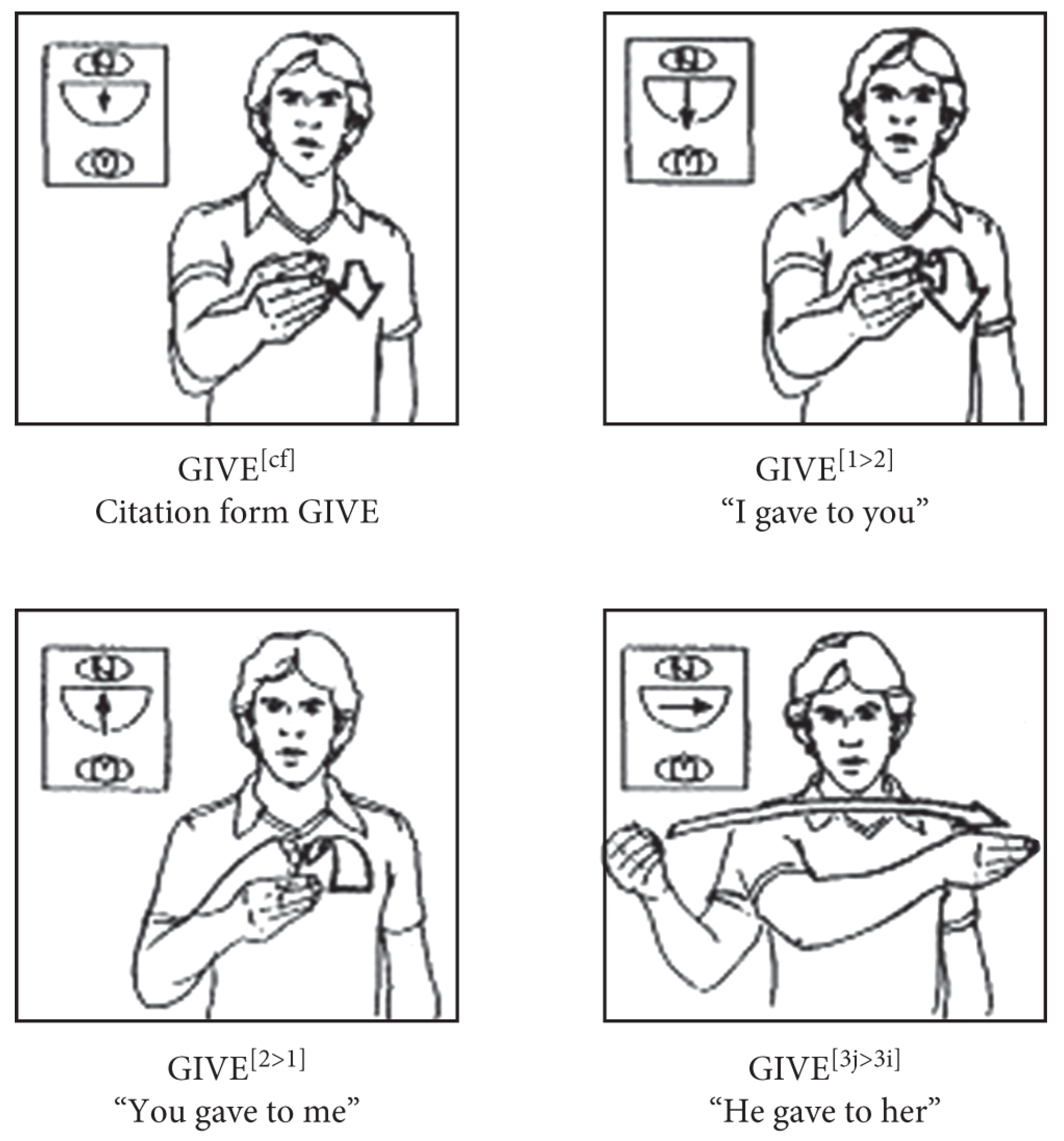
  • Fully Lexical Signs (FLSs): they correspond to the core of popular annotation systems. They are conventionalized units; a FLS may either be a content sign or a function sign (which roughly correspond to nouns and verbs in English). FLSs are identified by ID-glosses (Glossing is the practice of writing down a sign-by-sign equivalent using words (glosses) in English (or another written language). ID-glosses are more robust that simple glosses, as they are unique identifiers for the root morpheme of signs, which are unique identifiers, related to the form of the sign only, without consideration for meaning.
  • Partially Lexical Signs (PLSs): they are formed by the combination of conventional and non-conventional elements, the latter being highly context-dependent. Thus, they can not be listed in a dictionary. They include:
    -
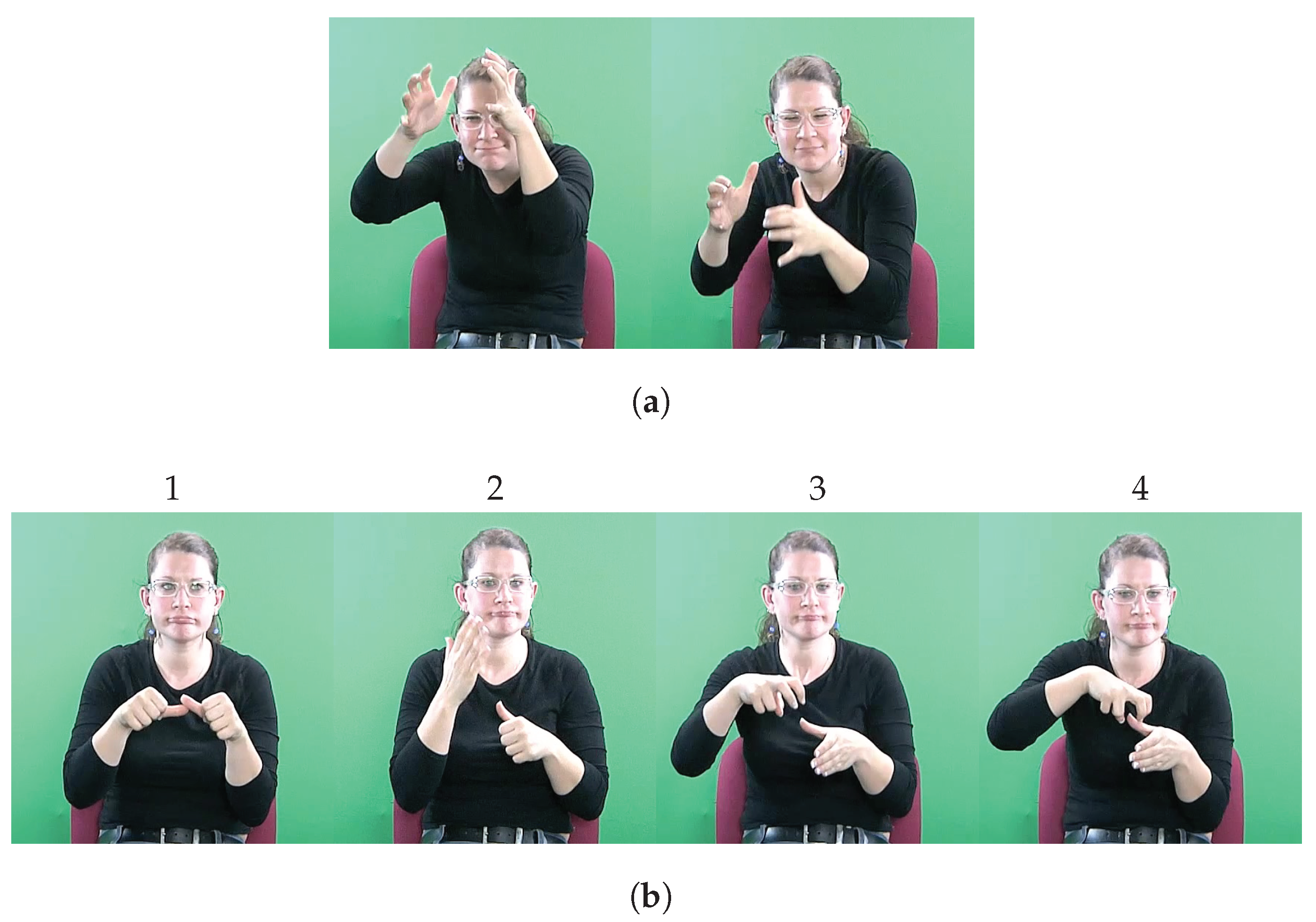
    Depicting Signs (DSs) or illustrative structures.
    -
    Pointing Signs (PTSs) or indexing signs.
    -
    Fragment Buoys (FBuoys) for the holding of a fragment or the final posture of a two-handed lexical sign, usually on the weak hand (i.e., the left hand for a right-handed person and vice versa).
  • Non Lexical Signs (NLSs), including Fingerspelled Signs (FSs) for proper names or when the sign is unknown, Gestures (Gs) for non-lexicalized gestures, which may be culturally shared or idiosyncratic, and Numbering Signs (NSs).
In the illustration sequence of Figure 3 from the Dicta-Sign–LSF–v2 corpus [8], three FLSs are produced (thumbnails 1, 2–3, 9), while thumbnails 4–8 correspond to a Highly Iconic Structure (Structure de Grande Iconicité). According to the typology of [2], thumbnails 4 and 5 correspond to a Situational Transfer—representing someone climbing up to the middle of the tower, while thumbnails 6 and 7 would be accurately described by a Transfer of Form and Size—representing the shape of a restaurant.
In a more general way, Sallandre et al. [9] have shown that taking PLSs into account is crucial for Sign Language Understanding (SLU): indeed, depending on the discourse type, the PLS:FLS ratio ranges from 1:4 to 4:1.
Based on this discussion about SL linguistics, it appears that various types of manual units should be dealt with by SLR systems. In the next section, we review the state-of-the-art in CSLR, which is in fact almost exclusively focused on recognizing FLSs.

1.2. Automatic Continuous Sign Language Recognition: State of the Art

In this article, we focus on Continuous Sign Language (CSL) only, leaving out the case of isolated signs, which does not involve any language processing. As a matter of fact, it appears that the vast majority of research experiments on CSL have focused on the recognition of lexical signs within a signed utterance, hence we refer to this approach as Continuous Lexical Sign Recognition (CLexSR).
Very specific corpora have become popular, which is detailed in Section 1.2.1. Then, we give an overview on the evolution of frameworks to tackle this research problem, along with associated results (Section 1.2.2). Experiments outside CLexSR are also discussed (Section 1.2.3).

1.2.1. Specific corpora used for Continuous Lexical Sign Recognition

Specific annotated SL corpora are used for this task, with lexical annotations only, with three of them standing out:
The German Sign Language (DGS) SIGNUM Database [10] contains 780 elicited sentences, based on 450 lexical signs. In total, there is approximately five hours of video. Because of the rigorous elicitation procedure, it is safe to say that the level of spontaneity as well as the interpersonal variability in the observed SL are very low. Signers indeed repeat the original reference sentences with no initiative. The elicited gloss sequences have lengths ranging from two to eleven glosses.
The RWTH-Phœnix-Weather (RWTH-PW) corpus [11,12,13] is made from 11 h of live DGS interpretation of weather forecast on German television, with nine interpreters. Conversely to many corpora produced in laboratory conditions and/or strong elicitation rules, RWTH-PW has been described by its authors as real-life data [11]. However, because of the specific topic, the language variability is necessarily limited. Furthermore, it is crucial to note that interpreted SL is a specific type of SL, quite different from spontaneous SL. There is a good chance that the translation will be strongly influenced by the original speech (in German), especially in terms of syntax, and make little use of the structures typical of SL [14].
The Continuous SLR100 (CSLR100) dataset [15] is a continuous Chinese Sign Language (ChSL) corpus, with more than 100 h of recordings. However, the level of variability and spontaneity in the produced language is very low: the corpus is based on 100 pre-defined sentences, that are repeated five times by 50 signers. In total, 25,000 sentences are thus recorded. The lexicon only amounts to 178 different lexical signs.

1.2.2. Continuous Lexical Sign Recognition Experiments: Frameworks and Results

Formally, starting from a SL video utterance, the problem of CLexSR consists in outputting a sequence of recognized lexical signs, as close as possible to the expected (annotated) sequence. The commonly associated performance metric is the Word Error Rate (WER), which measures the minimal number of insertions I, substitutions S and deletions D to turn the recognized sequence into the expected sequence of length N:
WER = I + S + D N .
The first identified challenge for CSLR—a fortiori for CLexSR— is the movement epenthesis, also called co-articulation: in a comparable way to what happens in natural speech, i.e., the transition between signs in natural SL is continuous, with a modification of the beginning and end of signs with respect to their standard form. Hidden Markov Models (HMMs) enable us to explicitly model the transition between signs in CSL. This is demonstrated first by [16], using data gloves, then by [17], with RGB video input.
An ongoing competition for the best CLexSR results on the RWTH-Phœnix-Weather corpus was then initiated by a sophisticated model presented by [13], with dynamic programming to track hands, HOG-3D features and inter-hand and facial features. They tested their model on both RWTH-PW and SIGNUM.
Thereafter, Convolutional Neural Networks (CNNs) have become more and more popular and predominantly used as an effective way to derive visual features. Koller et al. [18] embedded a CNN into an iterative Expectation Maximization (EM) algorithm in order to train Deep Hand, a powerful hand shape classifier, on weak labels. Training is realized on data from three SLs, namely DGS, New Zealand Sign Language (NZSL) and Danish Sign Language (DTS). Finally, the authors used Deep Hand instead of the HOG-3D for hand features in the model of [13], with improved results. Later, the authors built a unified CNN-HMM model, trained in an end-to-end fashion [19].
Similarly to [18,20] trained SubUNets, a CNN-BLSTM network trained for hand shape recognition and CLexSR, in an end-to-end fashion. The same kind of model is proposed by [21]. Koller et al. [22] then released a new model, consisting of embedding a CNN-BLSTM into a HMM, and treat the annotations as weak labels. Thanks to several EM re-alignments, the performance improves significantly, both on RWTH-PW and on SIGNUM, with WER of 26.8 % and 4.8 % on the respective signer-dependent test sets. Moreover, they also tested their model on the signer-independent version of RWTH-PW and obtained a WER of 44.1 % , which is a relative 65 % higher, showing that the signer-independence is a challenge that should not be overlooked.
Using two CNN streams—one for the hands and a global one—for feature extraction, [15] used a combination of Long Short-Term Memory (LSTM) and Attention [23] to tackle the temporal modality, with an encoder–decoder architecture, along with a Dynamic Time Warping (DTW) algorithm. They published results on RWTH-PW and the signer-independent version of the Continuous SLR100 dataset.
Recently, 3DCNNs have proven effective for action recognition, and have progressively replaced traditional 2D convolutions. The LSTM encoder–decoder architecture with Attention is used by [24,25], and Connectionist Temporal Classification (CTC) decoding by [25,26,27,28,29]. Guo et al. [26,27] also compute temporal convolutions.
Lastly, [30] used different sources of data to train a sophisticated multi-stream CNN-LSTM embedded into a HMM framework. They indeed trained the network to recognize lexical sign glosses, mouth shapes and hand shapes, in a weakly supervised fashion, with the three HMMs having to synchronize at the end of each sign.
Table 1 summarizes most CLexSR results on RWTH-PW, SIGNUM and CSLR100. From this table, it appears that most experiments are conducted in a signer-dependent fashion. Signer independence appears to be quite a challenge, with a best result of 44.1 % WER on RWTH-PW. This table confirms that RWTH-PW corresponds to the most difficult CLexSR task, whereas some models yield WERs lower than 5% on SIGNUM and CSLR100.

1.2.3. Experiments Outside the Field of Continuous Lexical Sign Recognition

As exemplified by Table 1, competition in the field of SLR is highly focused on the task of CLexSR, especially on the RWTH-PW corpus. However, it is notable that a few works have tried to explore the task of end-to-end Sign Language Translation, using the Neural Machine Translation (NMT) encoder–decoder architecture. However, the associated models are trained with a full [34] or partial [33] gloss supervision, on the quite linguistically restricted corpus RWTH-PW (see Section 1.2.1). Such models are thus ill-equipped to tackle natural SL utterances that include non-conventionalized illustrative structures.
While acceptable SLT performance is not nearly achieved, other SLR works have opted for more realistic goals and tackling some complex linguistics processes of SL. Very early on, [16] made use of data gloves to build a SLR system for the recognition of standard lexical signs, proforms and directional verbs. This HMM-based model was tested on a small self-made corpus, with encouraging results, although scaling up to bigger corpora with coarser annotation schemes is not straightforward. More recently, on the NCSLGR corpus (see below) [35] trained a HMM-SVM model to recognize five non-manual markers—in this case, face expressions—on a subset of the NCSLGR corpus, which are relevant at the syntactic level, namely: Negation, Wh-questions, Yes/no questions, Topic or focus and Conditional or ’when’ clauses. Related to this, [36] trained and tested a sign type classifier. Their model, based on optical flow and a Conditional Random Field (CRF) architecture, classifies any frame into one of three main sign types: Lexical sign, Fingerspelled sign and Classifier sign. The advertised accuracy is high (91.3% at the frame level), but it is computed on frames that belong to the three categories only.

1.3. Limitations of the Current Acceptation of Continuous Sign Language Recognition

In the previous discussion, we show that the current acceptation of CSLR is what we refer to as CLexSR, which is the recognition of lexical sign glosses within continuous signing. On the basis of strong linguistic arguments, it appears that this direction is strongly biased, and will not make it possible to go towards SLU and a fortiori to SLT. Indeed, the gloss sequence description misses main SL characteristics: the multilinearity, which makes it possible to convey several types of information at once; the prevalent use of space, which structures SL discourse; the iconicity, which enables us to show while saying.
Our point is hardly new, and has been put forward early on by a few researchers in the field of SLR. For instance, [16] insisted on the importance of space as a grammar component of French Sign Language (LSF). In another work, [37] mentioned complementary arguments, observing that the focus had been on conventional signs—gestures–leaving out the grammar of SL—primarily referring to the iconic characteristic of SLs, and the multilinear aspects of SL, like facial expression or body posture.
Related to the fact that CLexSR has been the main concern of researchers, leaving out the three linguistic characteristics we just mentioned, specific types of SL corpora have become popular. Many of them consist of artificial elicited sentences, repeated several times, with eliciting material—and annotation schemes—consisting of sequences of glosses. This is, for instance, the case of the SIGNUM Database and the CSLR100 corpus. Probably the most popular corpus, RWTH-PW is more spontaneous although the interpreted SL lacks generalizability and the topic—weather forecasts—is quite restricted.
Another limitation of using glosses as the training objective of SLR systems that should be noted, is the fact that glosses do not necessarily represent the meaning of signs they are associated to. This is highlighted by [6], warning that “used alone like this, glosses almost invariably distort face-to-face SL data”.
Independently, we appreciate that a few leads have been initiated towards different directions than CLexSR. SLT is one of them, although it has been mostly driven by gloss supervision, on the limitative RWTH-PW corpus. On the other hand, focusing on SLT or on the recognition of lexical signs only, with black box architectures, may prevent developments in the linguistic description and automatic analysis of SL. A few approaches have actually chosen to deal with linguistic matters, yet on very small corpora or only superficially.
In the next section, we propose a broader and more relevant acceptation of CSLR that deals with the aforementioned issues.

2. Materials and Methods

In this section, we introduce better corpora for CSLR (Section 2.1), a redefinition of CSLR (Section 2.2.1) with adapted metrics (Section 2.2.2) and a proposal for a generalizable and compact signer representation (Section 2.3.1) and learning framework (Section 2.3.2).

2.1. Better Corpora for Continuous Sign Language Recognition

2.1.1. A Few Corpora Made by Linguists

Conversely to SIGNUM, RWTH-PW and CSLR100, many SL corpora have been made by linguists. We introduce six of them: the Auslan Corpus [7], the BSL Corpus (BSLCP) [38], the DGS Korpus [39], the LSFB Corpus [40], the NCSLGR corpus [41] and Corpus NGT [42,43]. An overview of these corpora, along with those presented in Section 1.2.1, is given in Table 2. In this table, we include the number of signers, total duration, discourse type, and whether a written translation is included in the annotation as well as the annotation categories (besides lexical sign glosses).
Except for NCSLGR, these corpora are large in terms of duration, they include many signers and are made of dialogues, narratives and conversations. Undoubtedly, they can be considered very representative of natural SL. These corpora contain very interesting annotation information outside lexicon: PTSs for the Auslan Corpus, BSLCP and NCSLGR; DSs for the Auslan Corpus, BSLCP, the LSFB Corpus, Corpus NGT and NCSLGR; Constructed action for the Auslan Corpus; FBuoys for BSLCP; Mouthing for the DGS Korpus and Corpus NGT; FSs for NCSLGR. However, because these corpora have been made by linguists and intended for linguistic analysis, using them for SLR tasks is not straightforward. The main reason for this is the lack of consistency in the annotations across the corpora: most of them are still ongoing work, with annotations being updated continuously.
On the other hand, NCSLGR has consistent annotation across the corpus. However, this is not a dialogue corpus. Most utterances are artificial, furthermore the size of the corpus is small, with only two hours of recordings.

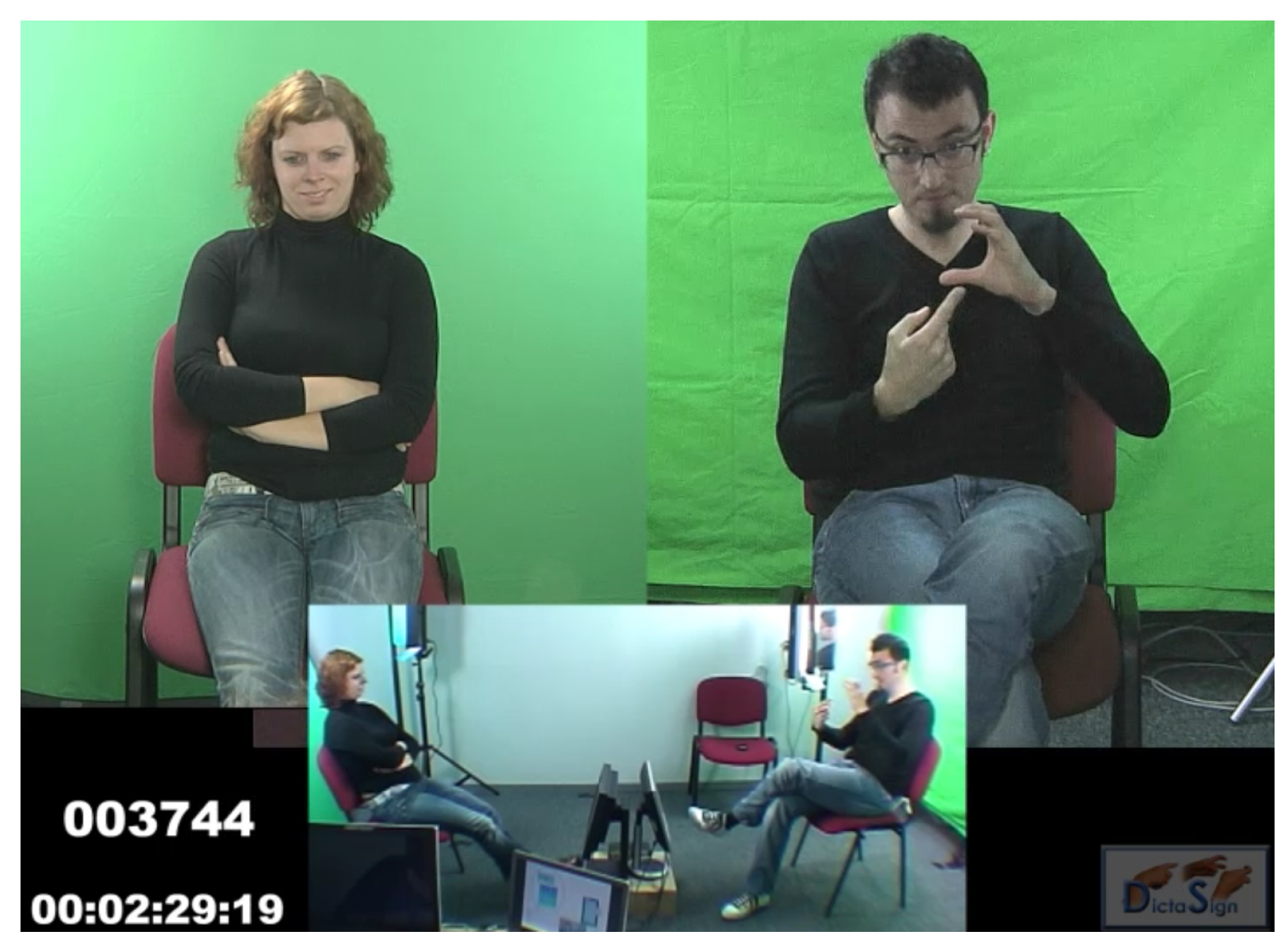
2.1.2. Dicta-Sign–LSF–v2: A Linguistic-Driven Corpus with Fine and Consistent Annotation

Mixing the best of both worlds, Dicta-Sign–LSF–v2 [44] is a very natural dialogue corpus made by linguists, with fine and consistent annotation across the 11 h of recordings of the corpus. It features annotation data for PTSs, DSs, FSs, FBuoys, NSs and Gs. Furthermore, the corpus is publicly available on the language platform Ortolang (https://hdl.handle.net/11403/dicta-sign-lsf-v2 [44]) (Ortolang is a platform for language, which aims at constructing an online infrastructure for storing and sharing language data (corpora, lexicons, dictionaries, etc.) and associated tools for its processing). The recording setup can be seen in Figure 4. The elicitation guidelines consisted in having the participants discuss about nine different topics about travel in Europe, i.e., nine different tasks.
The annotation categories are strongly influenced by the guidelines of [6] that are detailed in Section 1.1. All annotations are binary, except for FLS, which are annotated as a categorical variable. Annotations include: FLSs, PLSs (DSs, PTSs, FBuoys), NLSs (NSs, FSs and Gs). These categories are considered mutually exclusive, although one should note that ambiguity is often present. This is the case for some very iconic units that can be categorized as lexical signs but also as illustrative structures. Sign count distribution—for the FLSs—is shown in Table 3, while detailed statistics for all annotation categories are presented in Table 4.

2.2. Redefining Continuous Sign Language Recognition

2.2.1. Formalization

In order to formalize the general problem of SLR, let:
  • X = f 1 , , f T a SL video sequence of T frames.
  • R an intermediate representation of X, often called features.
  • M a learning and prediction model.
  • Y the element(s) of interest from X, that are to be recognized.
  • Y ^ an estimation of Y.
  • G = { g ( 1 ) , , g ( G ) } a dictionary of G lexical sign glosses.
The process of SLR can be seen as a function, or model, using R and M to estimate Y:
X R , M Y ^
The performance of such a model is then evaluated through a function P , which measures the discrepancy between Y and Y ^ , the objective being of course that Y ^ is as close as possible to Y:
P ( Y , Y ^ ) .
Obviously, the performance is always evaluated on videos unseen during training of both R and M . A crucial setting is the choice of signer-dependency: a signer-independent setting, in which tested signers are excluded from training videos, which makes learning a much harder task than a signer-dependent training, but also drastically increases the generalizability of the trained model.
The different categories of SLR rely on the form and content of X and Y. Within each category, different options can be considered for R , M and P . It is important to note that R and M , which is the representation of data and the learning-prediction model, are usually chosen in conjunction. Some learning architectures are indeed better adapted to some representations than others. Also, R and M are sometimes one and the same, for instance in the case of CNNs.

Case of CLexSR

The common acceptation of CSLR, which we refer to as CLexSR, corresponds to the recognition of the lexical sign glosses within the input video sequence X. Let us assume that X contains N consecutive lexical signs ( N 1 ). We assume N ^ lexical signs are recognized, such that:
Y CLexSR = g 1 g N , g i G Y ^ CLexSR = g ^ 1 g ^ N ^ , g ^ i G .
Note than in general, N N ^ , so Y CLexSR and Y ^ CLexSR have different lengths. Then, the usual sequence-wise recognition performance P CLexSR is usually defined as the WER, also referred to as Levenshtein Distance, applied to the expected sequences of lexical sign glosses (cf. Equation (1)).

Our Proposed Approach of General CSLR

Generally speaking, we propose interpreting CSLR as the continuous recognition of several linguistic descriptors. Let us consider such a CSLR acceptation with M different linguistic descriptors d m , m { 1 , , M } , so that Y CSLR can be written as:
Y CSLR = d 1 d M
with performance metric as a vector of size M, each descriptor having its own metric—or its set of metrics:
P ( Y , Y ^ ) = P 1 P M .
One may notice that CLexSR, as formalized previously, corresponds to the continuous recognition of one linguistic descriptor ( M = 1 ). The form of the unique descriptor d 1 is detailed in Equation (4).
Because we are considering continuous recognition, and without loss of generality, we suppose that all descriptors d m , m { 1 , , M } have a temporal dimension of length T, that is the original number of video frames (going from a frame-wise labeling of glosses to the usual gloss sequence Y CLexSR is straightforward, as it consists in removing duplicates and frames with no label). With this assumption, we can write:
Y CSLR = d 1 1 d T 1 d 1 M d T M .
As SLs are four-dimensional languages [45] (Sallandre, p. 103), with signs and realizations located not only in time but also in the three dimensions of space, each d t m ( m { 1 , , M } , t { 1 , , T } ) could also include spatial information—for instance they could be described by a vector of size 3, indicating the location of each sign realization. However, for sake of simplicity, and because we have no knowledge of a CSL corpus that would be annotated both in space and time, we consider each d t m as a scalar. Each of these scalars can be binary, categorical or continuous, depending on the associated information.
In Table 5, we give an example of fine CSLR, with d 1 encoding recognized FLSs —categorical— d 2 the presence/absence of DSs—binary— d 2 the presence/absence of PTSs—binary—and d 4 the presence/absence of FBuoys—binary.
Table 5. Illustration of common Continuous Lexical Sign Recognition (CLexSR) on the sequence example from Figure 5, as well as a proposal for Continuous Sign Language Recognition (CSLR), including Fully Lexical Signs (FLSs), and binary prediction for the presence or absence of Depicting Signs (DSs), Pointing Signs (PTSs) and Fragment Buoys (FBuoys). Here, the lexicon is G = { ( g 0 : NULL , ) g 1 : ABSURD , , g 312 : CENTER , , g 1243 : RESTAURANT , } .
SLR TypeRecognition Objective YMetrics P
Usual CLexSR g 312 g 1243 WER
CSLR: d 1 : FLSs d 2 : DSs d 3 : PTSs d 4 : FBuoys g 0 g 0 g 0 g 312 g 0 g 1243 g 0 g 0 g 0 1 1 1 0 1 0 1 1 1 0 0 1 0 0 0 0 0 0 0 0 0 0 0 1 1 1 1 P 1 : Acc P 2 : F 1 P 3 : F 1 P 4 : F 1

2.2.2. Relevant Metrics

Frame-Wise

Each categorical descriptor d m , like the continuous—aligned—recognition of FLS glosses, can be analyzed with a simple accuracy metric Acc m :
Acc m = 1 T t = 1 T 𝟙 ( d t m = d t m ^ ) = # correctly labeled frames T
where 𝟙 is the identity function. Of course, accuracy can also be used for binary descriptors, which is a specific case of categorical descriptor with two categories.
Binary descriptors, which can be seen as categorical with two possible values, often correspond—in our case—to relatively rare events, such that predicting the value “0” for all frames may correspond to a very high accuracy. In order to address this issue, one may resort to the calculation of precision P and recall R:
P m = TP TP + FP = t d t m d t m ^ t d t m ^
R m = TP TP + FN = t d t m d t m ^ t d t m
where TP, FP and FN stand for true positives, false positives and false negatives, respectively. These formula can actually be generalized to non-binary values, with the following definitions:
P m = t 𝟙 ( d t m = d t m ^ and d t m 0 ) t 𝟙 ( d t m ^ 0 )
R m = t 𝟙 ( d t m = d t m ^ and d t m 0 ) t 𝟙 ( d t m 0 )
The F1-score, defined as the harmonic mean of precision and recall, is then used as a trade-off metric for binary classification:
F 1 m = 2 ( P m ) 1 + ( R m ) 1 1 .
One advantage of F1-score is that the minimum of the two performance values is emphasized.

Unit-Wise

Although accurate temporal localization is aimed for, frame-wise performance metrics may not be perfectly informative. Indeed, because the start and end of each unit can be quite subjective, even a good recognition model can get poor frame-wise Acc, P, R, F1 etc., especially if the units are short, like in the case of PTSs (cf. Table 4). Unit-level metrics are then needed to get a better perspective on a system performance.
Let U G be the set of all ground-truth annotated units and U D that of all detected units. The notion of precision and recall for categorical values in a temporal sequence format can then be extended to units. True and false positives and negatives are counted with respect to two points of view: either analyzing each annotated unit—and deciding whether it is sufficiently close to any detected unit (or each detected unit) and deciding whether it is sufficiently close to any annotated unit, i.e., precision matches each unit of the detected list to one of the units in the ground truth list, whereas recall matches each unit of the ground truth to one of the units in the detection list. Modified versions of precision and recall are defined as follows:
P = # of correctly detected units w . r . t . U D # of detected units = 1 | U D | u d U D IsCorrectlyPredicted ( u d , U G )
R = # of correctly detected units w . r . t . U G # of annotated units = 1 | U G | u g U G IsCorrectlyPredicted ( u g , U D )
where IsCorrectlyPredicted is a counting function (values are 0 or 1). The F1-score is defined as in Equation (13). Then, we propose two ways of counting correct predictions:
  • Counting units within a certain temporal window t w : P w ( t w ) , R w ( t w ) and F1 w ( t w )
    First, we propose a rather straightforward counting function that consists of positively counting a unit u d U D if and only if there exists a unit of the same class in U G , within a certain margin (temporal window) t w —respectively, a unit u g U G is counted positively if and only if there exists a unit of the same class in U D , within a certain margin t w .
    In this configuration, precision, recall and F1-score are named P w ( t w ) , R w ( t w ) and F1 w ( t w ) .    
  • Counting units with thresholds t ¯ p and t ¯ r on their normalized temporal intersection: P p r ( t ¯ p , t ¯ r ) , R p r ( t ¯ p , t ¯ r ) and F1 p r ( t ¯ p , t ¯ r ) .
    The authors of [46] proposed and applied a similar but refined set of metrics, adapted for human action recognition and localization, both in space and time. Because our data are only labeled in time, we set aside the space metrics, although they would definitely be useful with adapted annotations. In this setting, P p r ( t ¯ p , t ¯ r ) and R p r ( t ¯ p , t ¯ r ) are calculated by finding the best matching units. For each unit u d in the list U D , one can define the best match unit in U G as the one maximizing the normalized temporal overlap between units (and a symmetric formula for the best match in U D of a unit u g ). The counting function between two units then returns a positive value if:
    • The number of frames that are part of both units is sufficiently large with respect to the number of frames in the detected set, i.e., the detected excess duration is sufficiently small.
    • The number of frames that are part of both units is sufficiently large with respect to the number frames in the ground truth set, i.e., a sufficiently long duration of the unit has been found.
    The main integrated metric can finally be defined as follows:
    I p r = 1 2 I p + I r = 1 2 0 1 F 1 ( t ¯ p , 0 ) d t ¯ p + 0 1 F 1 ( 0 , t ¯ r ) d t ¯ r .
    Other interesting values include P p r ( 0 , 0 ) , R p r ( 0 , 0 ) and F 1 p r ( 0 , 0 ) , which correspond to counting matches as units with at least one intersecting frame.
All equations and a complete derivation of both metrics are given in Appendix A, with an example in the case of binary classification.

2.3. Proposal for a Generalizable and Compact Continuous Sign Language Recognition Framework

While end-to-end frameworks are easier to set up and do not require any prior knowledge on the signer representation, they require more data and may not be easily generalizable. When signer representation and learning model are decoupled, the generalizability with respect to new types of videos are introduced, and one does not need to retrain the whole network in case new linguistic descriptors are added to the model. The reduced demand on training data is also an important benefit of such models, as annotated SL corpora are not that large. Also, the black box architecture of end-to-end models does not enable one to get a straightforward feedback on which signer features are linguistically relevant for recognition. We have thus chosen to resort to a separate approach. Section 2.3.1 details our proposal for a relevant, light and generalizable signer representation, then Section 2.3.2 outlines how such a signer representation can be coupled to a Recurrent Neural Network (RNN) for general CSLR.

2.3.1. Signer Representation

Since available training data are limited in quantity, we have decided to partly rely on pre-trained models for signer representation, with a separate processing of upper body, face and hands—which are usually dealt with in very specific ways, whether in SL-specific or non-SL-specific models.

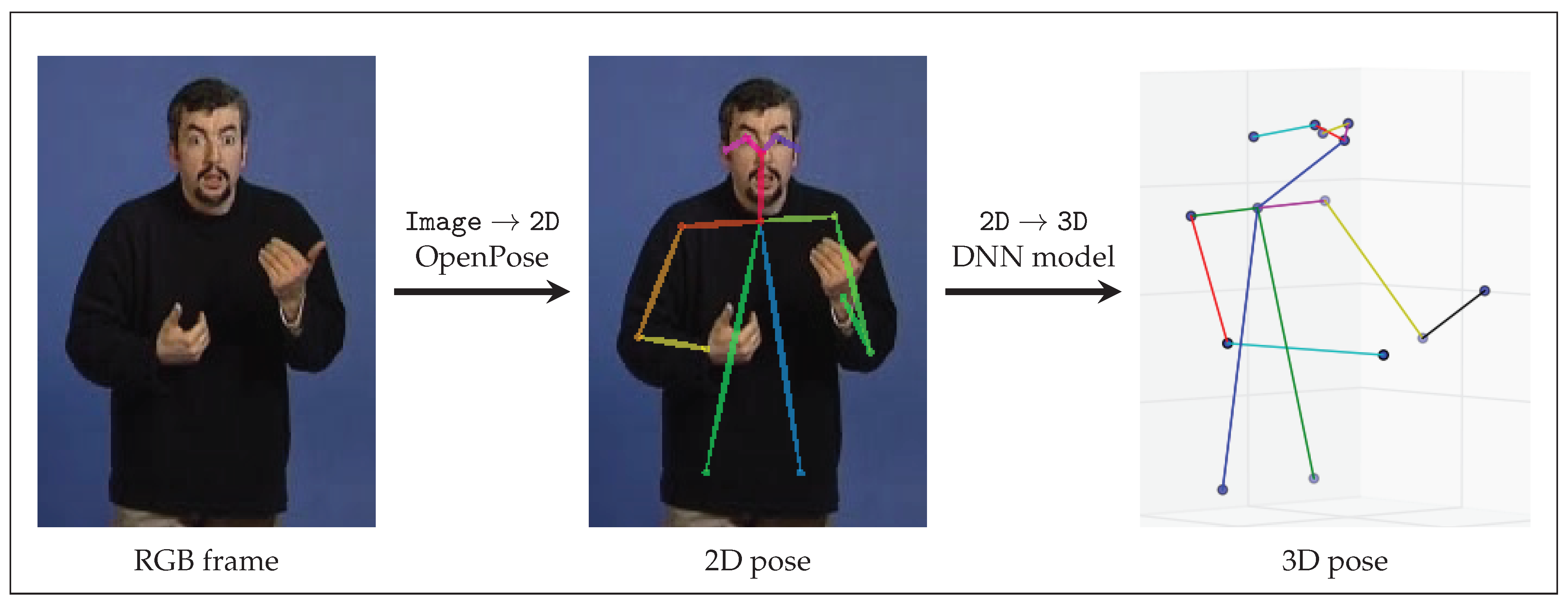
Upper Body: Image → 2D, Image → 3D, Image → 2D → 3D
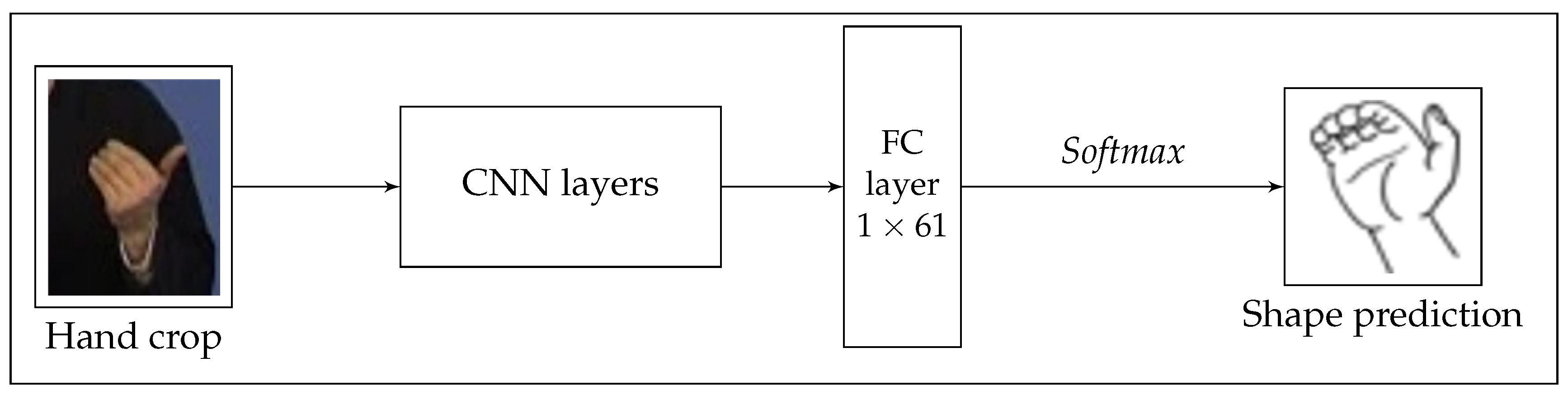
CNNs have emerged as a very effective tool to get relevant features from images. OpenPose (OP) [47,48] is a powerful open source library, with real-time capability for estimating 2D body pose. Widely used in the gesture recognition community, its Image → 2D body pose estimation module is fast—close to real-time for 25 frames per second (fps) videos on a modestly powerful desktop computer—is easy to use and works well even when part of the body is missing from the image—we only kept the 14 upper body keypoints and leave out the leg keypoints. This is a great benefit, as most SLs videos only show the upper body. Many other pose estimation models we have experimented on do not offer this feature.
Although direct Image → 3D models do exist (for instance [49]), we were not able to find one fitting our requirements. Indeed, as for Image → 2D models, prediction usually fails when part of the body is missing from the image, or when the person is not centered with respect to the image. Another type of issue is related to the training data of these models. As they were not trained with SL data, our experience is that they do not perform well when fed with SL images. Fortunately, the 2D OP estimates have proven robust even on SL videos. Therefore, we decided to rely on OP in order to get good 2D estimates, then train a 2D → 3D Deep Neural Network (DNN), reproducing the architecture from [50]. In the end, a Image → 2D → 3D model was thus obtained, aiming to learn the function f that estimates the third coordinate for each landmark of the signer in frame t, that is, with n as the number of landmarks ( n = 14 in our case):
f : | R 2 n R n ( x ^ 1 t , y ^ 1 t ) , ( x ^ 2 t , y ^ 2 t ) , , ( x ^ n t , y ^ n t ) z ^ 1 t , z ^ 2 t , , z ^ n t
where x ^ i t , y ^ i t and z ^ i t are a standardized version of the original coordinates x i t , y i t and z i t , with respect to the whole training dataset. The training loss is defined as the Euclidean distance between predictions and ground-truth data. The training data we decided to use for training consisted of motion capture data from the LSF corpus MOCAP1 [51]. These data have been particularly valuable since it contains high precision 3D landmarks recording of LSF, from four different signers. In order to increase model generalizability, data augmentation techniques were used during training. In detail, the 3D data from MOCAP1 were randomly rotated at each training epoch, with added pan Δ θ p 45 , + 45 , added tilt Δ θ t 20 , + 20 and added roll Δ θ r 5 , + 5 . The proposed DNN is implemented with Keras [52] on top of TensorFlow [53]. All hidden layers use Rectified Linear Unit activation [54], with Dropout to prevent overfitting [55]. RMSProp was used as the gradient optimizer [56]. Six neuron layers were stacked, with sizes [ 28 , 28 , 28 , 28 , 28 , 14 ] . The proposed Image → 2D → 3D pipeline for processing the 3D upper body pose from signers in RGB frames is shown in Figure 6.

Hands

Hands are obviously one of the main articulators in SL. Although linguists do not all share a common ground for the description and linguistic role of sub-units for the hands, three important parameters have been identified. More specifically—at least from an articulatory point of view—the location, shape and orientation of both hands are known to be critical, along with the dynamics of these three variables, that is: hand trajectory, shape deformation and hand rotation.
In addition to the body pose feature, the OP library also includes a Image → 2D hand pose estimation module, with RGB images as input [58]. From our experience, this module is quite sensitive to the image resolution, and even more to the video frame rate. Indeed, very poor results are obtained on blurred images, which is often the case for the hands with 25–30 fps videos in standard resolution. This is mostly due to the fact that hands can move fast in SL production, causing motion blur around the hands and forearms. Moreover, the hand shapes used in SL can be very sophisticated, and somehow never used in the daily life of non-signing people. Therefore, in all likelihood, the data that were used to train the OP models did not include such hand configurations, which sometimes makes predictions unreliable. That being said, the OP hand module can still be seen as a good and light proxy for hand representation. Let us note that although Image → 3D hand pose models have been developed (see for instance [49]), we have not found any that was able to provide a reliable estimate on hand pose on real-life 25 fps SL videos. Indeed, these models are even more sensitive to the issues encountered by the Image → 2D estimators.
An alternative direction is to extract global features from hand crops. Focusing on hand shape—thus setting aside location and orientation—a SL-specific model was developed in [18]. This CNN model classifies cropped hand images into 61 predefined hand shapes classes and was trained on more than a million frames, including motion blurred images. Three SL corpora of different types were compiled (Danish Sign Language (DTS), New Zealand Sign Language (NZSL), German Sign Language (DGS)). Even though the hand shapes frequency of occurrence is very likely to vary between different SLs, we have made the assumption that SLs other than DTS, NZSL and DGS could still be dealt with without retraining the model. Indeed, many hand shapes are obviously shared across most SLs, since they are used to depict salient and/or primary forms (flat, round, square, etc.). The trained prediction model 1-miohands-v2 is publicly available (https://www-i6.informatik.rwth-aachen.de/~koller/1miohands/), under the Caffe architecture [59]. A simplified scheme is presented in Figure 7. The input of the model is a cropped hand image, which was processed by several CNN layers. The final layer is of Fully Connected (FC) type, with 61 neurons, one for each class. The model outputs the most probable class with a softmax operation. However, we chose to extract the output of the last fully-connected layer and thus get a much more informative representation vector of size 61, for each hand, instead of the unique value corresponding to the most probable class.

Face and Head Pose

Similarly to body pose and to hand pose, the OP library makes it possible to get a 70-keypoint Image → 2D face pose estimate. Alternatively, a reliable 68-keypoint Image → 3D estimate is directly obtained from video frames thanks to a CNN model [60] trained on 230 , 000 images.

Final Signer Representation: From Raw Data to Relevant Features

With X as video frames, the final signer representation x = R ( X ) that we propose is simply a combination of:
  • the previously introduced raw data:
    • x shapes h a n d : vector of hand shapes probabilities for both hands, with size 122 ( 2 × 61 scalars per hand).
    • x raw 2 D h a n d : 2D raw hand pose vector, size 126 ( 2 × [21 2D landmarks plus 21 confidence scores]).
    • x raw 2 D b : 2D raw body pose vector, size 28 (14 2D landmarks).
    • x raw 3 D b : 3D raw body pose vector, size 42 (14 3D landmarks).
    • x raw 2 D f h : 2D raw face/head pose vector, size 140 (70 2D landmarks).
    • x raw 3 D f h : 3D raw face/head pose vector, size 204 (68 3D landmarks).
  • a relevant preprocessed body/face/head feature vector that can be used in combination with or as an alternative to raw data. Indeed, raw values are highly correlated, with a lot of redundancy, they can be difficult to interpret and are not always meaningful for SLR. We take inspiration from previous work in gesture recognition [61,62] and first compute pairwise positions and distances, as well as joint angles and orientations (wrist, elbow and shoulder), plus first and second order derivatives. In order to reduce the dimensionality of the face/head feature vector, the following components are computed: three Euler angles for the rotation of the head, plus first and second-order derivatives, mouth size (horizontal and vertical distances), relative motion of each eyebrow to parent eye center and position of nose landmark with respect to body center. The detection of contacts between hands and specific locations of the body is known to increase recognition accuracy [63]. Therefore, the feature vector also includes the relative position between each wrist and the nose, plus first and second-order derivatives. Moreover, because SLs make intensive use of hands, their relative arrangement is crucial [64]. Therefore, we also compute the relative position and distance of one wrist to the other, plus first and second order derivatives. We also derived a relevant 2D feature vector, in the same manner as the 3D one. In this case, positions, distances and angles are actually projected positions, distances and angles on the 2D plane. Finally, we get:
    • x feat 2 D b f h : 2D feature vector, size 96.
    • x feat 3 D b f h : 3D feature vector, size 176.

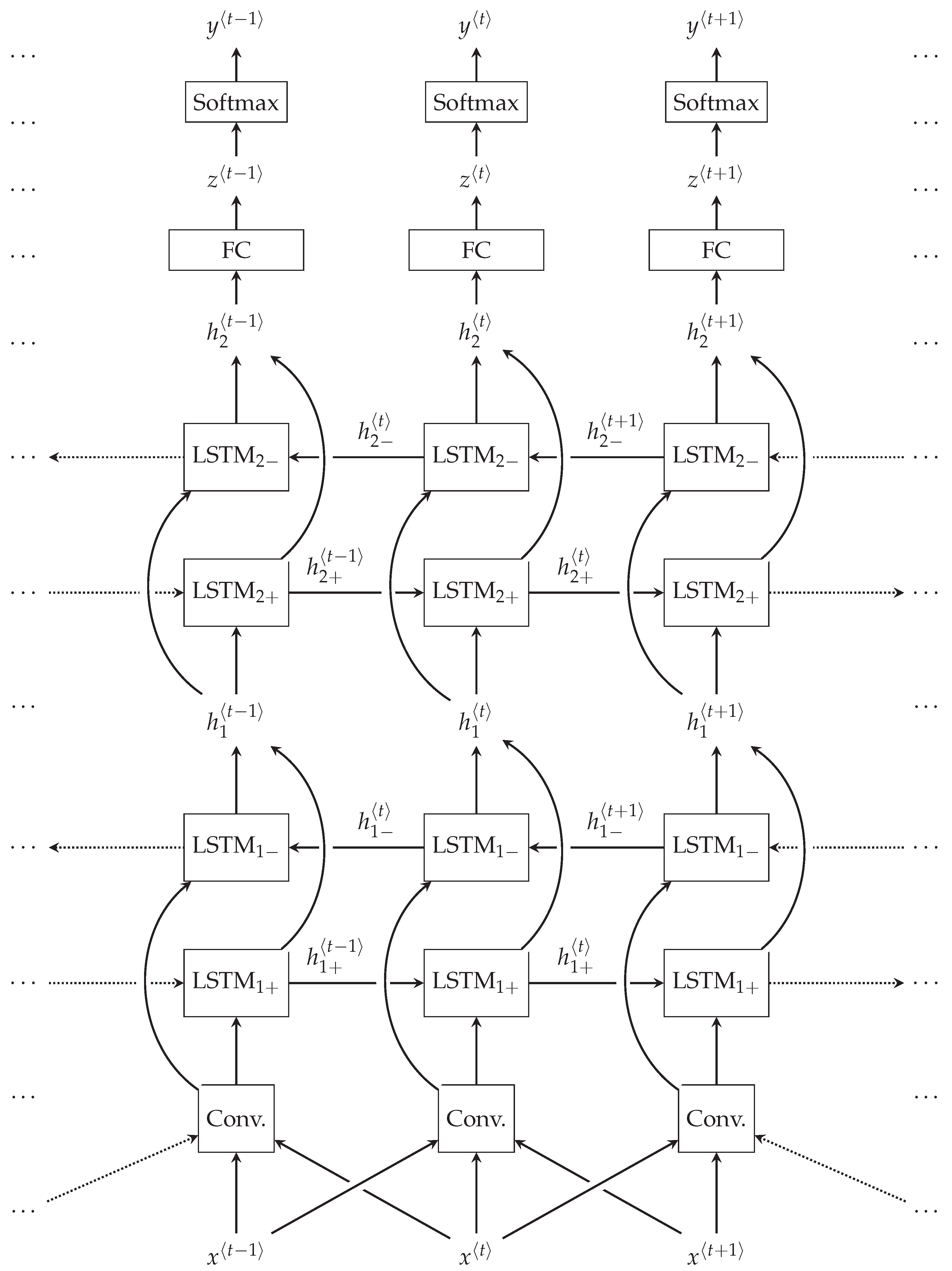
2.3.2. Learning Model

With a signer representation x = R ( X ) , setting up a learning and prediction model consists in defining M such that M ( x ) = Y ^ CSLR and Y ^ CSLR Y .
In Section 1.2.2, we present different types of learning frameworks taking one-dimensional time-series as input, which is our case. The most effective architectures used HMMs, CRFs and RNNs. In our experiments, we chose to use RNNs, mainly for the following reasons: they are good to build complex features from not always meaningful input, they are very modular and straightforward to train and they exhibit the best results in the field of Gesture Recognition (GR) and SLR. We used LSTMs units [65] that include a cell state c in addition to the usual hidden state h of RNNs. When real-time predictions are not needed, forward and backward LSTM units can be paired to form Bidirectional lstms (BLSTMs). Several layers of BLSTMs can then be stacked, as shown on Figure 8 detailing a two-layer BLSTM. Our experiments usually include one to four BLSTM layers.
An interesting addition for helping the network build relevant features is to set up the first layer as a one-dimensional temporal convolution. Temporal convolutions can help with noisy high-frequency data like ours, and are good to learn temporal dependencies [66]. A convolution layer with a kernel width of three frames is included on Figure 8.
Using the Keras library [52] on top of TensorFlow [53], we then built a modular architecture (https://github.com/vbelissen/cslr_limsi/) with a convolutional layer (with as parameters the number of filters and the kernel size), one or multiple LSTM or BLSTM layers (with as parameters the number of units), a FC layer and a final softmax operation for classification. Finally, the training phase is associated to many parameters as well, including the learning rate and optimizer, batch size, sequence length, dropout rate, data imbalance correction and the choice of metric.
In the next section, we aim to validate this proposal.

3. Results and Discussion

This section details our results in a series of CSLR experiments on the Dicta-Sign–LSF–v2 corpus. We decided to focus on the binary recognition of four manual unit types: FLSs, DSs, PTSs and FBuoys. These categories are representative of the variety of SL linguistic structures, with conventional and illustrative units, as well as elements highly used within the syntactic iconicity of SL. Other types show a too small number of instances for the results to be significant, or even for the network to converge (see detail in Table 4). First, we start with a quantitative assessment in Section 3.1, then, a more qualitative analysis on two test sequences of Dicta-Sign–LSF–v2 is outlined in Section 3.2.

3.1. Quantitative Assessment

In this first study, we present quantitative results of the proposed model. The chosen performance metrics and learning architecture parameters are detailed in Section 3.1.1, along with sixteen different signer representations. Baseline results for the most advanced representation are subsequently outlined in Section 3.1.2, enabling a fair comparison between the performance of the four proposed descriptors. Then, we end this study with more detailed results with respect to the influence of different signer representations (Section 3.1.3) and signer or task-independence (Section 3.1.4) on the recognition performance.

3.1.1. General Settings

Following the discussion of Section 2.2.2, the chosen performance metrics for validation include frame-wise and unit-wise measures, with detail, are presented below:
  • Frame-wise accuracy (not necessarily informative, as detailed in Section 2.2.2).
  • Frame-wise F1-score.
  • Unit-wise margin-based F1-score F1 w ( t w ) , with margin t w = 12 frames (half a second).
  • Unit-wise normalized intersection-based F1-score F 1 p r ( t ¯ p , t ¯ r ) , with t ¯ p = 0 , t ¯ r = 0 (counting positive recognition for units with at least one intersecting frame), as well as the associated integral value I p r .
All training sessions, unless otherwise specified, are conducted with the following common settings:
  • Network parameters: One BLSTM layer; 50 units in each LSTM cell; 200 convolutional filters as a first neural layer, with a kernel width of size 3.
  • Training hyperparameters: A batch size of 200 sequences; A dropout rate of 0.5; No weight penalty in the learning loss; Samples arranged with a sequence length of 100 frames.
  • The training loss is the weighted binary/categorical cross-entropy.
  • The gradient descent optimizer is RMSProp [56].
  • A cross-validation split of the data is realized in a signer-independent fashion, with 12 signers in the training set, 2 in the validation set and 2 in the test set.
  • Each run consists of 150 epochs. Only the best model was retained, in terms of performance on the validation set. During training, only the frame-wise F1-score was used to make this decision.
Furthermore, we defined 16 combinations of the feature vectors presented in Section 2.3.1. The detail of these configurations is given in Table 6, in which we also indicate the final representation vector size (for each frame), ranging from 218 for combination 5 to 494 for combination 9. Body and face data were either 2D or 3D, raw or made of preprocessed features, while hand data were made of OpenPose estimates, Deep Hand predictions or both.
In the following, we analyze the results for the signer representation #16, which usually gives best or close to best results. Then, we analyze the impact of varying the signer representation on the recognition results.

3.1.2. Baseline Results for Signer Representation #16

The results are summarized in Table 7, in which we report average values and standard deviation after seven identical simulations, for the binary recognition of FLSs, DSs, PTSs and FBuoys.
From this table, it appears that the best results are obtained for the recognition of FLSs, with a 64% frame-wise F1-score and a 52% I p r . DSs and PTSs get comparable performance values, while FBuoys are not very well recognized—14% frame-wise F1-score and 11% I p r . Except for FBuoys, one can note that the recall is usually higher than the precision, which means that there are more false positives than false negatives.
The differences in terms of performance can be explained first by the discrepancy with respect to the number of training instances: as can be seen in Table 4, FLSs account for about 75% of the manual units, while this drops to 11% for DSs and for PTSs. Only 589 FBuoy instances are annotated in Dicta-Sign–LSF–v2, that is about 2% of the total number of manual units.
However, other reasons can be proposed. DSs are a very broad category of units—many sub-categories can be listed—with a lot of inner variability. Also, the role of eye gaze is known to be crucial in DSs, however our signer representations include no gaze information. PTSs are very short, sometimes they last only one or two frames in 25 fps videos. As for FBuoys, they correspond to a maintained hand shape at the end of a bimanual sign, when it bears a linguistic function, which is not easy to detect (sometimes the hand shape is held for other reasons, and is not annotated as a FBuoy).

3.1.3. Influence of Signer Representation

Table 8 and Table 9 present the model performance metrics on the validation set, for each of the 16 combinations and each of the four different annotation types. In each table, one line corresponds to a particular combination, i.e., a certain signer representation. For each metric (except accuracy), the best setting is in bold. Not all metrics yield the same conclusion with respect to the best settings: in case of disagreement, we have used the integrated unit-wise metric I p r as decision rule, which is highlighted in the two tables. For instance, for the binary recognition of Fully Lexical Signs, the best combination—with an I p r of 0.60—is #15: 3D features, with hand shapes from the Deep Hand model. For Depicting Signs, best performance is reached by 2D features, with both OpenPose and hand shape data. Pointing Signs are better recognized with 3D features and both OpenPose and hand shape data. Last, Fragment Buoys should be recognized with 2D or 3D features, with OpenPose data alone.
A few general insights can be drawn from these results:
  • Using preprocessed data instead of raw values is always beneficial to the model performance, whatever the linguistic category. For linguistic annotations with few training instances like PTSs or FBuoys, the model is not even able to converge with raw data.
  • In the end, it appears that 3D estimates do not always improve the model performance, compared to 2D data. FLSs and FBuoys are better recognized when using 3D, while DSs and PTSs should be predicted using 2D data. However, this surprising result might stem from the limited quality of the 3D estimates that we used. True 3D data (instead of estimates trained on motion capture recordings) might indeed be more reliable thus beneficial in any case.
  • In terms of hand representation, it appears that the Deep Hand model is beneficial when recognizing FLSs, while OpenPose estimates alone correspond to the best choice—or very close to it—for the other linguistic categories. The fact that Deep Hand alone performs quite well for the recognition of FLSs and not for the other types of units could be explained by the fact that FLSs use a large variety of hand shapes, whereas other units like DSs use few hand shapes, but are rather very determined by the hand orientation, that is not captured by Deep Hand. In other words, it is likely that DSs give a more balanced importance to all hand parameters than FLSs.

3.1.4. Signer-Independence and Task-Independence

Because we are considering both the problem of signer-independence and that of task-independence, four cases are to be analyzed. We only consider tasks 1 to 8, as task 9 of Dicta-Sign–LSF–v2 corresponds to isolated signs.
Signer-dependent and task-dependent (SD-TD): 
we randomly pick 60% of the videos for training, 20% for validation and 20% for testing. Some signers and tasks are shared across the three sets.
Signer-independent and task-dependent (SI-TD): 
we randomly pick 10 signers for training, 3 signers for validation and 3 signers for testing. All tasks are shared across the three sets.
Signer-dependent and task-independent (SD-TI): 
we randomly pick five tasks for training, two tasks for validation and one task for testing. All signers are shared across the three sets.
Signer-independent and task-independent (SI-TI):  
we randomly pick eight signers for training, four signers for validation and four signers for testing; three tasks for training, three tasks for validation and two tasks for testing. This roughly corresponds to a 55%-27%-18% training–validation–testing split in terms of video count. Notably in this setting, a fraction of the videos has to be left out—videos that correspond to signers in the training set, and tasks in the other sets, etc. In the end, it is thus expected that the amount of training data is more likely to be a limiting factor than for the three previously described configurations.
The results—averaged out values from seven repeats—are summarized in Table 10, using the same performance metrics as before. Surprisingly, it appears that results for the configurations SD-TD, SI-TD and SD-TI perform relatively close, which supports the idea that the proposed signer representation and learning framework are good at generalizing to unseen signers and unseen tasks. The fact that performance is much lower in the SI-TI configuration thus suggests that the amount of training data is indeed a limiting factor in our case.

3.2. Qualitative Analysis on Test Set

Although performance metrics provide interesting insights on the results of the proposed model, a more qualitative analysis is needed. In this section, we analyze the prediction results of the proposed model, on two test sequences of Dicta-Sign–LSF–v2 (Video clips are visible at https://github.com/vbelissen/cslr_limsi/blob/master/Clips.md). The signer representation is decided from the optimization Table 8 and Table 9. The chosen setup is signer-independent and task-dependent (SI-TD). The test signers are then unknown both from the training and validation sets. These results complement preliminary analyses focused on DSs and developed in [67].
In this analysis, we have trained four binary descriptors, corresponding to FLSs, DSs, PTSs and FBuoys. In Figure 9 and Figure 10 we show, from top to bottom: a few key thumbnails, a proposed English translation, expert annotations for FLSs and PLSs—each on three tracks, corresponding to right-handed, two-handed or left-handed units—and model predictions. Because all descriptors are binary, a positive prediction is equivalent to a probability greater than 0.5.

Video S7_T2_A10, Frames 660–790 (Figure 9)

This is a longer and much more complex sequence with all four types of annotations—ten FLSs, two DSs, three PTSs and one FBuoy. We propose the following translation: “For you to decide between those two [touristic] options, I will present them one after the other, then we will also discuss prices.”. This sequence makes extensive use of space at the syntactic level. Indeed, the lexical sign HESITATE is used in context in quite an iconic fashion, with one hand corresponding to an option A and the other hand to another option B. Using pointing signs and a visible tilt in the upper body, as well as localized signs like EXPLAIN, the two options are sequentially referred to in a very spatial and visual way. FLSs are detected quite correctly, with an I p r of 0.60. Two pointing signs are detected, while one is missed. The two successive DSs are correctly detected, even though they are not segmented like the annotations. In the end of the sequence—and to a lesser extent the beginning—DSs are predicted by the model although they are not annotated. However, they do include a form of iconicity—as mentioned earlier, it is spatial iconicity used at the syntactic level. The unique FBuoy is not detected, resulting in I p r = 0 .

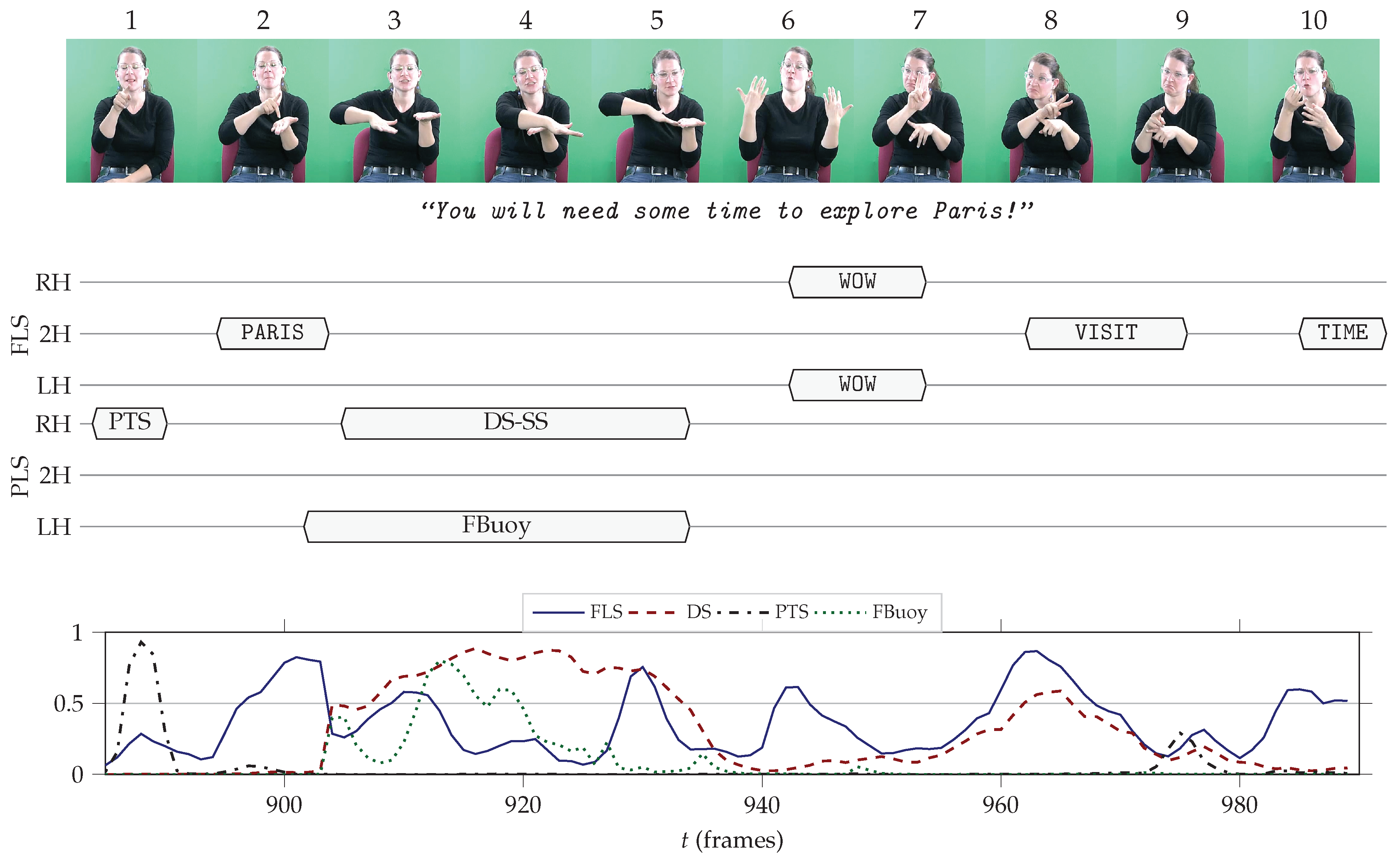
Video S7_T2_A10, Frames 885–990 (Figure 10)

This sequence is rather sequential and includes an illustrative structure around frame 920, with the left hand of the lexical sign PARIS iconically reactivated into a FBuoy, while the right hand performs a DS-Size&Shape (DS-SS). We propose the simple translation “You will need some time to explore Paris!”. All FLSs are detected correctly, but two false positives are observed in the vicinity of the illustrative structure. The unique PTS is perfectly recognized. The DS unit is very well detected too, while the simultaneous FBuoy is detected but much shorter than it is annotated. Interestingly, the FLS VISIT is also detected as a DS. This makes some sense as it is produced in quite an iconic way, in a form of Transfer of Persons (T-P), emphasized by the gaze moving away from the addressee and the crinkled eyes.
In conclusion to this qualitative assessment, it seems that the predictions of the four descriptors are generally well in line with the annotations, and could be used to describe a much broader part of SL discourse than the pure CLexSR approach. Moreover, many of the observed discrepancies can actually be explained by the subjectivity in the annotation, some annotation mistakes or even the unclear boundary between certain categories, in terms of linguistic definition—the FLS versus DS opposition may not always make sense, for instance; it may have been more appropriate to allow for both unit types to be positively annotated at the same time in the original corpus. More generally, the predictions of the proposed model could help question the exclusivity and relevance of certain linguistic categories. This will however require an even more thorough analysis of the results in order to ensure that no erroneous conclusions are drawn due to shortcomings in the signer representation or learning model.

4. Conclusions

In this work, we have first focused on improving the input data for CSLR systems, proposing Dicta-Sign–LSF–v2, a LSF corpus previously made by linguists. We then developed a general description of the problem of CSLR with adapted metrics. In order to realize a first series of experiments with this broader definition of CSLR, we have introduced and implemented an original combination of signer representation and learning model, using a mix of publicly available and self-developed models and a convolutional and recurrent neural network.
Finally, we have conducted a thorough analysis of the recognition performance of the proposed model for four very different linguistic descriptors—FLSs, DSs, PTSs and FBuoys—on Dicta-Sign–LSF–v2. We have shown that promising performance values are met. A qualitative analysis on the test set then illustrates the merits of the proposed approach.
As regards perspectives of this work, signer representation—in particular with respect to hand modeling—shows a lot of room for improvement. Independently, gathering quality annotated SL data is a major challenge, as the amount of training data appears to be a bottleneck for the performance of CSLR models.

Author Contributions

Conceptualization, V.B., A.B. and M.G.; methodology, V.B., A.B. and M.G.; software, V.B.; validation, V.B., A.B. and M.G.; formal analysis, V.B.; investigation, V.B., A.B. and M.G.; resources, A.B. and M.G.; data curation, V.B. and A.B.; writing—original draft preparation, V.B.; writing—review and editing, V.B., A.B. and M.G.; visualization, V.B., A.B. and M.G. supervision, A.B. and M.G.; project administration, A.B. and M.G.; funding acquisition, A.B. All authors have read and agreed to the published version of the manuscript.

Funding

This research received no external funding.

Conflicts of Interest

The authors declare no conflict of interest.

Abbreviations

The following abbreviations are used in this manuscript:
Machine Learning and Image Processing
BLSTMBidirectional LSTM
CNNConvolutional Neural Network
CRFConditional Random Field
CTCConnectionist Temporal Classification
DNNDeep Neural Network
DTWDynamic Time Warping
EMExpectation Maximization
FCFully Connected
fpsframes per second
HMMHidden Markov Model
HOGHistogram of Oriented Gradients
LSTMLong Short-Term Memory
NMTNeural Machine Translation
OPOpenPose [47]   
RCNNRecurrent Convolutional Neural Network
RGBRed-Green-Blue
RNNRecurrent Neural Network
SVMSupport Vector Machine
WERWord Error Rate
 
Sign Language
ASLAmerican Sign Language
ChSLChinese Sign Language
CLexSRContinuous Lexical Sign Recognition
CSLContinuous Sign Language
CSLRContinuous Sign Language RecognitionAlgorithms
DGSGerman Sign Language (Deutsche Gebärdensprache)
DTSDanish Sign Language (Dansk Tegnsprog)
GRGesture Recognition
HSHand shape
LSFFrench Sign Language (Langue des Signes Française)
NZSLNew Zealand Sign Language
SDSigner-Dependent (see signer-dependent)
SGIHighly Iconic Structure (Structure de Grande Iconicité) [68]
SISigner-Independent (see signer-independent)
SLSign Language
SLRSign Language Recognition
SLTSign Language Translation
SLUSign Language Understanding
TDTask Dependent
TITask Independent
T-SSituational Transfer
T-PTransfer of Persons
T-FSTransfer of Form and Size
 
Sign Language annotation categories
FLSFully Lexical Sign
 
PLSPartially Lexical Sign
DSDepicting Sign
DS-LDS-Location (of an entity)
DS-MDS-Motion (of an entity)
DS-SSDS-Size&Shape (of an entity)
DS-GDS-Ground (spatial or temporal reference)
PTSPointing Sign
FBuoyFragment Buoy
 
NLSNon Lexical Sign
FSFingerspelled Sign
NSNumbering Sign
GGesture

Appendix A. Performance Metrics for Temporal Data: Details and Illustration

In this appendix, we give more detailed equations and illustrate the performance metrics presented in Section 2.2.2. We choose the case of binary classification, with a dummy sequence for which fictitious annotated and predicted data are given in Figure A1.
Figure A1. Annotated (top, blue) and predicted (bottom, red) data in a dummy binary classification problem. Four units are annotated, while three are detected.
Algorithms 13 00310 g0a1

Appendix A.1. Frame-Wise Metrics

The frame-wise metrics are easily computed. We remind that U G corresponds to the set of all ground-truth annotated units and U D to that of all detected units. First, the accuracy is the rate of correctly predicted frames, including class 0: Acc = 0.61 .
Frame-wise precision and recall are computed from the count of true positives, false positives and false negatives frames (see Equations (9) and (10)): P = 15 15 + 11 0.58 and R = 15 15 + 28 0.35 which yield F 1 0.44 .

Appendix A.2. Unit-Wise Metrics
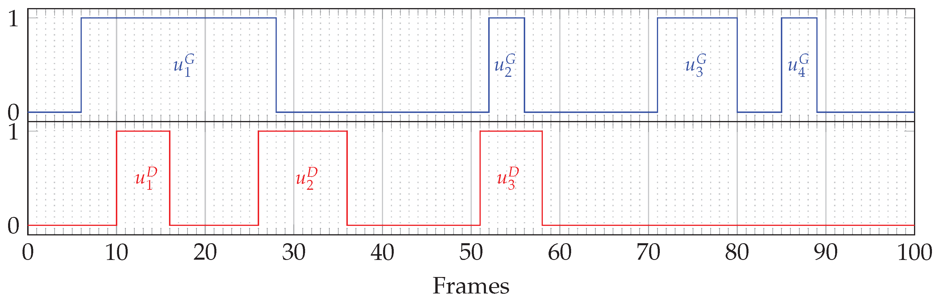
Appendix A.2.1. P w , R w , F 1 w

For these metrics, the time gap between the middle of u d and the middle of the closest unit of the same class in U G is compared to t w , in order to decide whether u d is a correct detection–respectively, the time gap between the middle of u g and the middle of the closest unit of the same class in U D is compared to t w , in order to decide whether u g is correctly detected. Let us first note that:
  • The closest unit from u 1 D is unit u 1 G , with 4 frames of shift between their respective centers.
  • The closest unit from u 2 D is unit u 1 G , with 14 frames of shift between their respective centers.
  • The closest unit from u 3 D is unit u 2 G , with 0.5 frame of shift between their respective centers.
Also:
  • The closest unit from u 1 G is unit u 1 D , with 4 frames of shift between their respective centers.
  • The closest unit from u 1 G is unit u 3 D , with 0.5 frame of shift between their respective centers.
  • The closest unit from u 3 G is unit u 3 D , with 21 frames of shift between their respective centers.
  • The closest unit from u 4 G is unit u 3 D , with 32.5 frames of shift between their respective centers.
From Equations (14) and (15), unit-wise precision and recall as a function of a margin t w can be written as:
P w ( t w ) = 1 3 𝟙 t w > 4 + 𝟙 t w > 14 + 𝟙 t w > 0.5 R w ( t w ) = 1 4 𝟙 t w > 4 + 𝟙 t w > 0.5 + 𝟙 t w > 21 + 𝟙 t w > 32.5 .
With margins of half a second (12 frames) or one second (25 frames), numerical values are:
P w ( 12 ) 0.67 ; R w ( 12 ) = 0.5 ; F 1 w ( 12 ) 0.57
and
P w ( 25 ) = 1 ; R w ( 25 ) = 0.75 ; F 1 w ( 25 ) 0.86 .

Appendix A.2.2. P Pr , R Pr , F 1 Pr

P p r ( t ¯ p , t ¯ r ) and R p r ( t ¯ p , t ¯ r ) can be expressed as:
P p r ( t ¯ p , t ¯ r ) = 1 | U D | u d U D IsMatched BestMatch u d , U G , u d , t ¯ p , t ¯ r )
R p r ( t ¯ p , t ¯ r ) = 1 | U G | u g U G IsMatched u g , BestMatch u g , U D , t ¯ p , t ¯ r ) .
For each unit u d in the list U D , one can define the best match unit in U G as the one maximizing the normalized temporal overlap between units (and a symmetric formula for the best match of a unit u g in U D ):
BestMatch u d , U G = argmax u g U G 2 # frames u g u d # frames u g + # frames u d if Class ( u g ) = Class ( u d ) 0 otherwise
IsMatched decides whether two units are sufficiently similar, which can be written down as follows:
IsMatched u g , u d , t ¯ p , t ¯ r = 1 if # frames u g u d # frames u d > t ¯ p # frames u g u d # frames u g > t ¯ r Class ( u g ) = Class ( u d ) 0 otherwise .
From Equations (A3) and its symmetric, one can note that:
  • The best match for unit u 1 D is unit u 1 G , with 7 intersecting frames over the 7 frames of u 1 D .
  • The best match for unit u 2 D is unit u 1 G , with 3 intersecting frames over the 11 frames of u 2 D .
  • The best match for unit u 3 D is unit u 2 G , with 5 intersecting frames over the 8 frames of u 3 D .
Also:
  • The best match for unit u 1 G is unit u 1 D , with 10 intersecting frames over the 23 frames of u 1 G .
  • The best match for unit u 2 G is unit u 3 D , with 5 intersecting frames over the 5 frames of u 2 G .
  • The best match for unit u 3 G is any unit u i D , because there is no intersection.
  • The best match for unit u 4 G is any unit u i D , because there is no intersection.
Then, with IM standing for IsMatch, P p r and R p r of Equations (A1) and (A2) can be simply expressed as:
P p r ( t ¯ p , t ¯ r ) = 1 3 IM ( u 1 D , u 1 G , t ¯ p , t ¯ r ) + IM ( u 2 D , u 1 G , t ¯ p , t ¯ r ) + IM ( u 3 D , u 2 G , t ¯ p , t ¯ r ) = 1 3 𝟙 { 7 7 > t ¯ p , 7 23 > t ¯ r } + 𝟙 { 3 11 > t ¯ p , 3 23 > t ¯ r } + 𝟙 { 5 8 > t ¯ p , 5 5 > t ¯ r } R p r ( t ¯ p , t ¯ r ) = 1 4 IM ( u 1 D , u 1 G , t ¯ p , t ¯ r ) + IM ( u 3 D , u 2 G , t ¯ p , t ¯ r ) + IM ( u i D , u 3 G , t ¯ p , t ¯ r ) + IM ( u i D , u 4 G , t ¯ p , t ¯ r ) = 1 4 𝟙 { 7 7 > t ¯ p , 7 23 > t ¯ r } + 𝟙 { 5 8 > t ¯ p , 5 5 > t ¯ r } + 0 + 0 .
These formula make it possible to draw curves for P p r , R p r and F 1 p r , either with fixed t ¯ r = 0 or fixed t ¯ p = 0 . This is shown in Figure A2. The calculation of area under curves (Equation (16)) then yields:
I p r 0.438 .
Figure A2. Unit-wise P p r , R p r and F 1 p r values, in the case of the dummy sequences of Figure A1, as a function of t ¯ p ( t ¯ r = 0 ), or as a function of t ¯ r ( t ¯ p = 0 ).
Algorithms 13 00310 g0a2

References

  1. Stokoe, W.C. Sign Language Structure: An Outline of the Visual Communication Systems of the American Deaf. Studies in Linguistics. Stud. Linguist. 1960, 8, 269–271. [Google Scholar]
  2. Cuxac, C. French Sign Language: Proposition of a Structural Explanation by Iconicity. In Proceedings of the 1999 International Gesture Workshop on Gesture and Sign Language in Human-Computer Interaction; Springer: Berlin, Germany, 1999; pp. 165–184. [Google Scholar]
  3. Pizzuto, E.A.; Pietrandrea, P.; Simone, R. Verbal and Sign Languages. Comparing Structures, Constructs, Methodologies; Mouton De Gruyter: Berlin, Germany, 2007. [Google Scholar]
  4. Liddell, S.K. An Investigation into the Syntactic Structure of American Sign Language; University of California: San Diego, CA, USA, 1977. [Google Scholar]
  5. Meier, R.P. Elicited imitation of verb agreement in American Sign Language: Iconically or morphologically determined? J. Mem. Lang. 1987, 26, 362–376. [Google Scholar] [CrossRef]
  6. Johnston, T.; De Beuzeville, L. Auslan Corpus Annotation Guidelines; Centre for Language Sciences, Department of Linguistics, Macquarie University: Sydney, Australia, 2014. [Google Scholar]
  7. Johnston, T. Creating a corpus of Auslan within an Australian National Corpus. In Proceedings of the 2008 HCSNet Workshop on Designing the Australian National Corpus, Sydney, Australia, 4–5 December 2008. [Google Scholar]
  8. Belissen, V.; Gouiffès, M.; Braffort, A. Dicta-Sign-LSF-v2: Remake of a Continuous French Sign Language Dialogue Corpus and a First Baseline for Automatic Sign Language Processing. In Proceedings of the 12th International Conference on Language Resources and Evaluation (LREC 2020), Marseille, France, 11–16 May 2020. [Google Scholar]
  9. Sallandre, M.A.; Balvet, A.; Besnard, G.; Garcia, B. Étude Exploratoire de la Fréquence des Catégories Linguistiques dans Quatre Genres Discursifs en LSF. Available online: https://journals.openedition.org/lidil/7136 (accessed on 24 November 2020).
  10. Von Agris, U.; Kraiss, K.F. Towards a Video Corpus for Signer-Independent Continuous Sign Language Recognition. In Proceedings of the 2007 International Gesture Workshop on Gesture and Sign Language in Human-Computer Interaction, Lisbon, Portugal, 23–25 May 2007. [Google Scholar]
  11. Forster, J.; Schmidt, C.; Hoyoux, T.; Koller, O.; Zelle, U.; Piater, J.H.; Ney, H. RWTH-PHOENIX-Weather: A Large Vocabulary Sign Language Recognition and Translation Corpus. In Proceedings of the 8th International Conference on Language Resources and Evaluation (LREC 2012), Istanbul, Turkey, 21 May 2012. [Google Scholar]
  12. Forster, J.; Schmidt, C.; Koller, O.; Bellgardt, M.; Ney, H. Extensions of the Sign Language Recognition and Translation Corpus RWTH-PHOENIX-Weather. In Proceedings of the 9th International Conference on Language Resources and Evaluation (LREC 2014), Reykjavik, Iceland, 26–31 May 2014. [Google Scholar]
  13. Koller, O.; Forster, J.; Ney, H. Continuous Sign Language Recognition: Towards Large Vocabulary Statistical Recognition Systems Handling Multiple Signers. Comput. Vis. Image Underst. 2015, 141, 108–125. [Google Scholar] [CrossRef]
  14. Metzger, M. Sign Language Interpreting: Deconstructing the Myth of Neutrality; Gallaudet University Press: Washington, DC, USA, 1999. [Google Scholar]
  15. Huang, J.; Zhou, W.; Zhang, Q.; Li, H.; Li, W. Video-based Sign Language Recognition without Temporal Segmentation. In Proceedings of the 32nd AAAI Conference on Artificial Intelligence, New Orleans, LA, USA, 2–7 February 2018. [Google Scholar]
  16. Braffort, A. Reconnaissance et Compréhension de Gestes, Application à la Langue des Signes. Ph.D. Thesis, Université de Paris XI, Orsay, France, 28 June 1996. [Google Scholar]
  17. Vogler, C.; Metaxas, D. Adapting Hidden Markov Models for ASL Recognition by Using Three-dimensional Computer Vision Methods. In Proceedings of the 1997 IEEE International Conference on Systems, Man, and Cybernetics. Computational Cybernetics and Simulation, Orlando, FL, USA, 12–15 October 1997. [Google Scholar]
  18. Koller, O.; Ney, H.; Bowden, R. Deep Hand: How to Train a CNN on 1 Million Hand Images When Your Data is Continuous and Weakly Labelled. In Proceedings of the 2016 IEEE Conference on Computer Vision and Pattern Recognition (CVPR), Las Vegas, NV, USA, 27–30 June 2016. [Google Scholar]
  19. Koller, O.; Zargaran, S.; Ney, H.; Bowden, R. Deep Sign: Hybrid CNN-HMM for Continuous Sign Language Recognition. In Proceedings of the 2016 British Machine Vision Conference (BMVC), York, UK, 19–22 September 2016. [Google Scholar]
  20. Camgoz, N.C.; Hadfield, S.; Koller, O.; Bowden, R. SubUNets: End-to-End Hand Shape and Continuous Sign Language Recognition. In Proceedings of the 2017 IEEE International Conference on Computer Vision (ICCV), Venice, Italy, 22–29 October 2017. [Google Scholar]
  21. Cui, R.; Liu, H.; Zhang, C. Recurrent Convolutional Neural Networks for Continuous Sign Language Recognition by Staged Optimization. In Proceedings of the 2017 IEEE Conference on Computer Vision and Pattern Recognition (CVPR), Honolulu, HI, USA, 21–26 July 2017. [Google Scholar]
  22. Koller, O.; Zargaran, S.; Ney, H. Re-Sign: Re-Aligned End-to-End Sequence Modelling with Deep Recurrent CNN-HMMs. In Proceedings of the 2017 IEEE Conference on Computer Vision and Pattern Recognition (CVPR), Honolulu, HI, USA, 21–26 July 2017. [Google Scholar]
  23. Luong, T.; Pham, H.; Manning, C.D. Effective Approaches to Attention-based Neural Machine Translation. In Proceedings of the 2015 Conference on Empirical Methods in Natural Language Processing; Association for Computational Linguistics: Lisbon, Portugal, 2015; pp. 1412–1421. [Google Scholar] [CrossRef] [Green Version]
  24. Guo, D.; Zhou, W.; Li, H.; Wang, M. Hierarchical LSTM for Sign Language Translation. In Proceedings of the 32nd AAAI Conference on Artificial Intelligence, New Orleans, LA, USA, 2–7 February 2018. [Google Scholar]
  25. Pu, J.; Zhou, W.; Li, H. Iterative Alignment Network for Continuous Sign Language Recognition. In Proceedings of the 2019 IEEE Conference on Computer Vision and Pattern Recognition (CVPR), Long Beach, CA, USA, 15–21 June 2019. [Google Scholar]
  26. Guo, D.; Tang, S.; Wang, M. Connectionist Temporal Modeling of Video and Language: A Joint Model for Translation and Sign Labeling. In Proceedings of the 28th International Joint Conference on Artificial Intelligence; AAAI Press: Palo Alto, CA, USA, 2019. [Google Scholar]
  27. Guo, D.; Wang, S.; Tian, Q.; Wang, M. Dense Temporal Convolution Network for Sign Language Translation. In Proceedings of the 28th International Joint Conference on Artificial Intelligence; AAAI Press: Palo Alto, CA, USA, 2019. [Google Scholar]
  28. Yang, Z.; Shi, Z.; Shen, X.; Tai, Y.W. SF-Net: Structured Feature Network for Continuous Sign Language Recognition. arXiv 2019, arXiv:1908.01341. [Google Scholar]
  29. Zhou, H.; Zhou, W.; Li, H. Dynamic Pseudo Label Decoding for Continuous Sign Language Recognition. In Proceedings of the 2019 IEEE International Conference on Multimedia and Expo (ICME), Shanghai, China, 8–12 July 2019. [Google Scholar]
  30. Koller, O.; Camgoz, C.; Ney, H.; Bowden, R. Weakly Supervised Learning with Multi-Stream CNN-LSTM-HMMs to Discover Sequential Parallelism in Sign Language Videos. IEEE Trans. Pattern Anal. Mach. Intell. 2019, 42, 2306–2320. [Google Scholar] [CrossRef] [PubMed] [Green Version]
  31. Von Agris, U.; Knorr, M.; Kraiss, K.F. The Significance of Facial Features for Automatic Sign Language Recognition. In Proceedings of the 2008 8th IEEE International Conference on Automatic Face & Gesture Recognition, Amsterdam, The Netherlands, 17–19 September 2008. [Google Scholar]
  32. Koller, O.; Zargaran, S.; Ney, H.; Bowden, R. Deep Sign: Enabling Robust Statistical Continuous Sign Language Recognition via Hybrid CNN-HMMs. Int. J. Comput. Vis. 2018, 126, 1311–1325. [Google Scholar] [CrossRef] [Green Version]
  33. Camgoz, N.C.; Koller, O.; Hadfield, S.; Bowden, R. Sign Language Transformers: Joint End-to-end Sign Language Recognition and Translation. In Proceedings of the 2020 IEEE Conference on Computer Vision and Pattern Recognition (CVPR), Seattle, WA, USA, 16–18 June 2020. [Google Scholar]
  34. Camgoz, N.C.; Hadfield, S.; Koller, O.; Ney, H.; Bowden, R. Neural Sign Language Translation. In Proceedings of the 2018 IEEE Conference on Computer Vision and Pattern Recognition (CVPR), Salt Lake City, UT, USA, 18–22 June 2018. [Google Scholar]
  35. Metaxas, D.N.; Liu, B.; Yang, F.; Yang, P.; Michael, N.; Neidle, C. Recognition of Nonmanual Markers in American Sign Language (ASL) Using Non-Parametric Adaptive 2D-3D Face Tracking. In Proceedings of the 8th International Conference on Language Resources and Evaluation (LREC 2012), Istanbul, Turkey, 23 May 2012. [Google Scholar]
  36. Yanovich, P.; Neidle, C.; Metaxas, D.N. Detection of Major ASL Sign Types in Continuous Signing For ASL Recognition. In Proceedings of the 10th International Conference on Language Resources and Evaluation (LREC 2016), Portorož, Slovenia, 23 May 2012. [Google Scholar]
  37. Edwards, A.D. Progress in Sign Language Recognition. In Proceedings of the 1997 International Gesture Workshop on Gesture and Sign Language in Human-Computer Interaction; Springer: Berlin, Germany, 1997; pp. 13–21. [Google Scholar]
  38. Schembri, A. British Sign Language Corpus Project: Open Access Archives and the Observer’s Paradox. In Proceedings of the Language Resources and Evaluation Conference, Marrakech, Morocco, 28–30 May 2008. [Google Scholar]
  39. Prillwitz, S.; Hanke, T.; König, S.; Konrad, R.; Langer, G.; Schwarz, A. DGS Corpus Project-Development of a Corpus Based Electronic Dictionary German Sign Language/German. In Proceedings of the Satellite Workshop to the 6th International Conference on Language Resources and Evaluation (LREC 2008), Marrakech, Morocco, 26–27 May 2008. [Google Scholar]
  40. Meurant, L.; Sinte, A.; Bernagou, E. The French Belgian Sign Language Corpus A User-Friendly Searchable Online Corpus. In Proceedings of the 7th workshop on the Representation and Processing of Sign Languages: Corpus Mining, Portorož, Slovenia, 23–28 May 2016. [Google Scholar]
  41. Neidle, C.; Vogler, C. A New Web Interface to Facilitate Access to Corpora: Development of the ASLLRP Data Access Interface (DAI). Available online: https://www.ucviden.dk/en/publications/workshop-proceedings-5th-workshop-on-the-representation-and-proce (accessed on 24 November 2020).
  42. Crasborn, O.A.; Zwitserlood, I. The Corpus NGT: An Online Corpus for Professionals and Laymen. In Proceedings of the 3rd Workshop on the Representation and Processing of Sign Languages: Construction and Exploitation of Sign Language Corpora. Satellite Workshop to the 6th International Conference on Language Resources and Evaluation (LREC 2008); ELRA: Paris, France, 2008; pp. 44–49. [Google Scholar]
  43. Crasborn, O.; Zwitserlood, I.; Ros, J. Corpus NGT. In An Open Access Digital Corpus of Movies with Annotations of Sign Language of the Netherlands (Video Corpus). Centre for Language Studies, Radboud University Nijmegen. 2008. Available online: http://www.ru.nl/corpusngtuk (accessed on 24 November 2020).
  44. LIMSI; IRIT. Dicta-Sign-LSF-v2. Available online: https://hdl.handle.net/11403/dicta-sign-lsf-v2 (accessed on 24 November 2020).
  45. Vermeerbergen, M.; Leeson, L.; Crasborn, O. Simultaneity in Signed Languages: Form and Function; John Benjamins Publishing: Amsterdam, The Netherlands, 2007. [Google Scholar]
  46. Wolf, C.; Lombardi, E.; Mille, J.; Celiktutan, O.; Jiu, M.; Dogan, E.; Eren, G.; Baccouche, M.; Dellandréa, E.; Bichot, C.E.; et al. Evaluation of video activity localizations integrating quality and quantity measurements. Comput. Vis. Image Underst. 2014, 127, 14–30. [Google Scholar] [CrossRef] [Green Version]
  47. Cao, Z.; Simon, T.; Wei, S.E.; Sheikh, Y. Realtime Multi-Person 2D Pose Estimation using Part Affinity Fields. In Proceedings of the 2017 IEEE Conference on Computer Vision and Pattern Recognition (CVPR), Honolulu, HI, USA, 21–26 July 2017. [Google Scholar]
  48. Wei, S.E.; Ramakrishna, V.; Kanade, T.; Sheikh, Y. Convolutional Pose Machines. In Proceedings of the 2016 IEEE Conference on Computer Vision and Pattern Recognition (CVPR), Las Vegas, NV, USA, 27–30 June 2016. [Google Scholar]
  49. Xiang, D.; Joo, H.; Sheikh, Y. Monocular Total Capture: Posing Face, Body, and Hands in the Wild. In Proceedings of the 2018 IEEE Conference on Computer Vision and Pattern Recognition (CVPR), Salt Lake City, UT, USA, 18–22 June 2018. [Google Scholar]
  50. Zhao, R.; Wang, Y.; Benitez-Quiroz, C.F.; Liu, Y.; Martinez, A.M. Fast and Precise Face Alignment and 3D Shape Reconstruction from a Single 2D Image. In Proceedings of the 2016 European Conference on Computer Vision (ECCV); Springer: Berlin, Germany, 2016; pp. 590–603. [Google Scholar]
  51. LIMSI; CIAMS. MOCAP1. Available online: https://hdl.handle.net/11403/mocap1/v1 (accessed on 24 November 2020).
  52. Chollet, F. Keras. 2015. Available online: https://keras.io (accessed on 24 November 2020).
  53. Abadi, M.; Barham, P.; Chen, J.; Chen, Z.; Davis, A.; Dean, J.; Devin, M.; Ghemawat, S.; Irving, G.; Isard, M.; et al. Tensorflow: A system for large-scale machine learning. In Proceedings of the 12th USENIX Symposium on Operating Systems Design and Implementation (OSDI 16), Savannah, GA, USA, 2–4 November 2016. [Google Scholar]
  54. Nair, V.; Hinton, G.E. Rectified Linear Units Improve Restricted Boltzmann Machines. In Proceedings of the 27th International Conference on Machine Learning (ICML10), Haifa, Israel, 21–24 June 2010. [Google Scholar]
  55. Srivastava, N.; Hinton, G.; Krizhevsky, A.; Sutskever, I.; Salakhutdinov, R. Dropout: A Simple Way to Prevent Neural Networks from Overfitting. J. Mach. Learn. Res. 2014, 15, 1929–1958. [Google Scholar]
  56. Tieleman, T.; Hinton, G. Lecture 6.5—RmsProp: Divide the gradient by a running average of its recent magnitude. COURSERA Neural Netw. Mach. Learn. 2012, 4, 26–31. [Google Scholar]
  57. Braffort, A.; Choisier, A.; Collet, C.; Cuxac, C.; Dalle, P.; Fusellier, I.; Gherbi, R.; Jausions, G.; Jirou, G.; Lejeune, F.; et al. Projet LS-COLIN. Quel Outil de Notation pour Quelle Analyse de la LS. Available online: https://www.irit.fr/publis/TCI/Dalle/rlsf01_LS_COLIN.pdf (accessed on 24 November 2020).
  58. Simon, T.; Joo, H.; Matthews, I.; Sheikh, Y. Hand Keypoint Detection in Single Images using Multiview Bootstrapping. In Proceedings of the 2017 IEEE Conference on Computer Vision and Pattern Recognition (CVPR), Honolulu, HI, USA, 21–26 July 2017. [Google Scholar]
  59. Jia, Y.; Shelhamer, E.; Donahue, J.; Karayev, S.; Long, J.; Girshick, R.; Guadarrama, S.; Darrell, T. Caffe: Convolutional Architecture for Fast Feature Embedding. In Proceedings of the 22nd ACM international conference on Multimedia, Utrecht, The Netherlands, 25–29 October 2020. [Google Scholar]
  60. Bulat, A.; Tzimiropoulos, G. How far are we from solving the 2D & 3D Face Alignment problem? (and a dataset of 230,000 3D facial landmarks). In Proceedings of the 2017 IEEE International Conference on Computer Vision (ICCV), Venice, Italy, 22–29 October 2017. [Google Scholar]
  61. Granger, N.; el Yacoubi, M.A. Comparing Hybrid NN-HMM and RNN for Temporal Modeling in Gesture Recognition. In Proceeding of Advances in Neural Information Processing Systems (NIPS 2017); Springer: Berlin, Germany, 2017; pp. 147–156. [Google Scholar]
  62. Wu, D.; Pigou, L.; Kindermans, P.J.; Le, N.D.H.; Shao, L.; Dambre, J.; Odobez, J.M. Deep Dynamic Neural Networks for Multimodal Gesture Segmentation and Recognition. IEEE Trans. Pattern Anal. Mach. Intell. 2016, 38, 1583–1597. [Google Scholar] [CrossRef] [PubMed] [Green Version]
  63. Dilsizian, M.; Metaxas, D.; Neidle, C. Linguistically-driven Framework for Computationally Efficient and Scalable Sign Recognition. In Proceedings of the 11th International Conference on Language Resources and Evaluation (LREC 2018), Miyazaki, Japan, 7–12 May 2018. [Google Scholar]
  64. Battison, R. Phonological Deletion in American Sign Language. Sign Lang. Stud. 1974, 5, 1–19. [Google Scholar] [CrossRef]
  65. Gers, F.A.; Schmidhuber, J.; Cummins, F. Learning to Forget: Continual Prediction with LSTM. Neural Comput. 2000, 12, 2451–2471. [Google Scholar] [CrossRef] [PubMed]
  66. Pigou, L.; Van Den Oord, A.; Dieleman, S.; Van Herreweghe, M.; Dambre, J. Beyond Temporal Pooling: Recurrence and Temporal Convolutions for Gesture Recognition in Video. Int. J. Comput. Vis. 2018, 126, 430–439. [Google Scholar] [CrossRef] [Green Version]
  67. Belissen, V.; Gouiffès, M.; Braffort, A. Improving and Extending Continuous Sign Language Recognition: Taking Iconicity and Spatial Language into account. In Proceedings of the 9th Workshop on the Representation and Processing of Sign Languages: Sign Language Resources in the Service of the Language Community, Technological Challenges and Application Perspectives, Marseille, France, 11–16 May 2020. [Google Scholar]
  68. Cuxac, C. La Langue des Signes Française (LSF): Les Voies de l’Iconicité. Available online: https://pascal-francis.inist.fr/vibad/index.php?action=getRecordDetail&idt=238688 (accessed on 24 November 2020).
Figure 1. Examples of transfers in Highly Iconic Structures (Structures de Grande Iconicité), according to the typology of [2], most commonly referred to as Depicting Signs. (a) Transfer of Form and Size. The signer draws a sketch in space, representing the surface of an object with her hands. The shape of her lips and cheeks, her partially closed eyes and her lowered head emphasize the imposing character of this object. (b) Transfer of Persons (bored person) mixed with a Situational Transfer in frames 3 and 4 (going round and round in circles). The signer enacts a bored person, which is particularly visible on her face expression (cheeks and lips), her gaze looking away and her head moving side to side. In frames 3 and 4, the weak (left) hand depicts a reference point (corner of a room), while the dominant (right) hand uses a specific proform to represent a person, which illustrates a person going round and round in circles.
Algorithms 13 00310 g001
Figure 2. Citation form (i.e., standard form) and several variations of the directional verb GIVE[5], illustrating the use of space in the construction of discourse in SL.
Algorithms 13 00310 g002
Figure 3. LSF sequence from Dicta-Sign–LSF–v2 (video reference: S7_T2_A10). Expert annotations for right-handed (RH), two-handed (2H) and left-handed (LH) Fully Lexical Signs (FLSs) and Partially Lexical Signs (PLSs) are given.
Algorithms 13 00310 g003
Figure 4. Recording setup in Dicta-Sign–LSF–v2, with two frontal cameras and a side one.
Algorithms 13 00310 g004
Figure 5. French Sign Language sequence from Dicta-Sign–LSF–v2 (video reference: S7_T2_A10). Expert annotations for right-handed (RH), two-handed (2H) and left-handed (LH) Fully Lexical Signs (FLSs) and Partially Lexical Signs (PLSs) are given.
Algorithms 13 00310 g005
Figure 6. Proposed Image → 2D → 3D pipeline for the upper body pose, applied to a random frame from the French Sign Language corpus LS-COLIN [57]. OpenPose enables to get 2D estimates, then a DNN model was used to estimate the missing third coordinate of each landmark.
Algorithms 13 00310 g006
Figure 7. Synoptic architecture for the 1-miohands-v2 model from [18]. Hand crop images are processed by several Convolutional Neural Network (CNN) layers, then a final Fully Connected (FC) layer enables to estimate probabilities for each of the 61 classes, with a softmax operation.
Algorithms 13 00310 g007
Figure 8. Unrolled representation of a two-layer Bidirectional lstm (BLSTM) network for temporal classification, with input x and output y. The cell state c is omitted, for sake of clarity. Upstream of the LSTM layers, the input is first convolved, with a convolution kernel width of three frames on this scheme.
Algorithms 13 00310 g008
Figure 9. LSF sequence from Dicta-Sign–LSF–v2 (video reference: S7_T2_A10). Expert annotations for right-handed (RH), two-handed (2H) and left-handed (LH) Fully Lexical Signs (FLSs) and Partially Lexical Signs (PLSs) are given.
Algorithms 13 00310 g009
Figure 10. LSF sequence from Dicta-Sign–LSF–v2 (video reference: S7_T2_A10). Expert annotations for right-handed (RH), two-handed (2H) and left-handed (LH) Fully Lexical Signs (FLSs) and Partially Lexical Signs (PLSs) are given.
Algorithms 13 00310 g010
Table 1. Reported Word Error Rate (WER) (%) of methods detailed in Section 1.2.2 applied to Continuous Lexical Sign Recognition on the corpora presented in Section 1.2.1. SD and SI stand for Signer-Dependent and Signer-Independent. The exact same annotated sentences are present in training and test sets. It is unclear whether the training/test splits of the different papers are comparable.
PaperRWTH-Phœnix-WeatherSIGNUMContinuous SLR100
SDSISDSISDSI
Von Agris et al. [31]-- 12.7 34 . 9 --
Koller et al. [13] 53.0 - 10.0 ---
Koller et al. [18] 45.1 - 7.6 ---
Koller et al. [19] 38.8 - 7.4 ---
Camgoz et al. [20] 40.7 -----
Cui et al. [21] 38.7 -----
Koller et al. [22] 26.8 44 . 1 4 . 8 ---
Koller et al. [32] 32.5 - 7.4 ---
Huang et al. [15] 38.3 ---- 17.3
Guo et al. [24]---- 63.0 10.2
Pu et al. [25] 36.7 --- 32 . 7 -
Guo et al. [26] 38.7 --- 61.9 -
Guo et al. [27] 36.5 --- 44.7 14.3
Zhou et al. [29] 34.5 ---- 4.5
Yang et al. [28] 34.9 ---- 3 . 8
Koller et al. [30] 26.0 -----
Camgoz et al. [33] 24 . 5 -----
Table 2. Continuous Sign Language datasets. The top corpora have been developed and used by the SLR community, but they are either artificial or not representative of natural Sign Language. Others have been built by linguists, with natural discourse and detailed annotation, although they are not always consistent. To the best of our knowledge, Dicta-Sign–LSF–v2 and NCSLGR are the only two corpora built by linguists that have been used for beyond gloss-level CSLR experiments.
Corpus (SL)SignersHrs.Discourse TypeTranslationAnnotation Outside LexiconUsed for
CategoriesConsistent
[15] CSLR100 (ChSL)50100Artificial--SLR
[11] RWTH-PW (DGS)911InterpretedGerman-SLR
[10] SIGNUM (DGS)255ArtificialGer./Eng.-SLR
[41] NCSLGR (ASL)72Mixed-PTSs, DSs, FSsYesSLR & linguistics
[7] Auslan Corpus100150Natural-PTSs, DSs, Constructed actionNoLinguistics
[38] BSLCP249180NaturalEnglishPTSs, DSs, FBuoysNoLinguistics
[39] DGS Korpus33050–300NaturalGer./Eng.MouthingNoLinguistics
[40] LSFB Corpus100150NaturalFrenchDSsNoLinguistics
[42] Corpus NGT9272NaturalDutchDSs, MouthingNoLinguistics
[8] Dicta-Sign–LSF–v21611NaturalFrenchPTSs, DSs, FSs, FBuoys, NSs, GsYesSLR & linguistics
Table 3. Numbers derived from the cumulative distribution of the number of occurrences for the Fully Lexical Signs of Dicta-Sign–LSF–v2. The way this table can be read is, for instance: 1789 signs have less than or exactly 20 occurrences, while 292 signs have more than 20 occurrences.
# of Occurrences# of Signs with a Smaller or Equal # of Occurrences# of Signs with a Greater # of Occurrences
002081
15851496
101556525
201789292
50199784
100205130
20020729
40020801
Table 4. Frame count and sign count (manual unit) statistics for the main annotation categories of Dicta-Sign–LSF–v2.
FLSPLSNLSTotal
DSPTSFBuoyNSFS
Non blank frames20553060794230451435938301941309,499
%66.4%19.7%7.5%4.6%1.2%0.6%
Cumulative %66.4%86.1%93.6%98.2%99.4%100.0%
manual-unit245653606365158915511832,684
%75.2%11.0%11.2%1.7%0.5%0.4%
Cumulative %75.2%86.2%97.4%99.1%99.6%100.0%
Avg. frames/unit8.416.86.324.424.716.4
Avg. duration (ms)335674252975988658
Table 6. Detail of the 16 signer representations that are compared in Section 2.3.1.
# ConfigurationCorresponding Feature Vectors and Size (Section 2.3.1)Total Size
Body and Face Hands x raw 2 D b x raw 3 D b x raw 2 D fh x raw 3 D fh x raw 2 D hand x shapes hand x feat 2 D bfh x feat 3 D bfh
OPHS284214020412612296176
12DRaw 168
2 294
3 290
4 416
5Features 96
6 222
7 218
8 344
93DRaw 246
10 372
11 368
12 494
13Features 176
14 302
15 298
16 424
Table 7. Average ( μ ) and standard deviation ( σ ) values from seven identical simulations for the binary recognition of Fully Lexical Signs, Depicting Signs, Pointing Signs and Fragment Buoys, for the signer representation #16, on the validation set of Dicta-Sign–LSF–v2. Metrics displayed are frame-wise accuracy and F1-score, as well as unit-wise margin-based F1-score F1 w ( t w ) , with margin t w = 12 frames (half a second) and normalized intersection-based F1-score F 1 p r ( 0 , 0 ) (counting positive recognition for units with at least one intersecting frame).
Frame-WiseUnit-Wise
AccF1 (P/R)F 1 w ( t w = 12 ) (P/R)F 1 pr ( 0 , 0 ) (P/R) I pr
FLS μ 0.830.64 (0.56/0.74)0.86 (0.76/0.98)0.78 (0.65/0.98)0.52
σ 0.010.01 (0.02/0.02)0.02 (0.02/0.03)0.04 (0.05/0.01)0.03
DS μ 0.950.40 (0.35/0.49)0.48 (0.36/0.74)0.44 (0.32/0.72)0.31
σ 0.010.04 (0.07/0.08)0.06 (0.07/0.06)0.06 (0.07/0.06)0.04
PTS μ 0.970.31 (0.41/0.26)0.46 (0.40/0.56)0.45 (0.39/0.55)0.33
σ 0.010.02 (0.07/0.05)0.04 (0.06/0.10)0.05 (0.06/0.11)0.03
FBuoy μ 0.980.14 (0.25/0.10)0.13 (0.12/0.15)0.19 (0.22/0.18)0.11
σ 0.010.04 (0.07/0.04)0.03 (0.02/0.05)0.04 (0.05/0.05)0.03
Table 8. Performance assessment on the validation set of Dicta-Sign–LSF–v2, for different signer representations, applied to the recognition of FLSs and DSs. Each line corresponds to a particular signer representation, see Table 6. Bold values correspond to the best value for each setting category. In the end, I p r is used to decide the best representation.
Frame-WiseUnit-Wise
Body and Face HandsAccF1 (P/R)F 1 w ( t w = 12 ) (P/R)F 1 pr ( 0 , 0 ) (P/R) I pr
OPHS
Fully Lexical Sign   2DRaw 0.800.58 (0.51/0.68)0.57 (0.75/0.46)0.75 (0.76/0.73)0.42
0.790.16 (0.44/0.10)0.45 (0.87/0.30)0.34 (0.68/0.23)0.19
0.820.55 (0.56/0.55)0.83 (0.85/0.80)0.75 (0.76/0.74)0.45
0.800.19 (0.52/0.12)0.60 (0.86/0.46)0.42 (0.61/0.32)0.26
Features 0.860.68 (0.65/0.71)0.88 (0.81/0.97)0.78 (0.66/0.94)0.56
0.850.66 (0.61/0.73)0.85 (0.75/0.99)0.79 (0.67/0.98)0.57
0.840.63 (0.60/0.66)0.87 (0.78/0.99)0.75 (0.61/0.96)0.49
0.850.69(0.60/0.82)0.87 (0.78/0.98)0.81 (0.69/0.98)0.59
3DRaw 0.810.42 (0.56/0.34)0.68 (0.81/0.59)0.57 (0.64/0.52)0.32
0.820.47 (0.59/0.40)0.82 (0.82/0.82)0.64 (0.65/0.64)0.40
0.830.45 (0.64/0.34)0.73 (0.87/0.62)0.62 (0.76/0.52)0.38
0.800.37 (0.51/0.29)0.73 (0.83/0.66)0.58 (0.66/0.51)0.34
Features 0.830.65 (0.55/0.78)0.84 (0.73/0.99)0.73 (0.59/0.97)0.51
0.870.69(0.66/0.73)0.89 (0.81/0.98)0.80 (0.69/0.95)0.57
0.860.69(0.64/0.75)0.90(0.82/0.99)0.83(0.73/0.97)0.60
0.830.64 (0.56/0.74)0.86 (0.76/0.98)0.78 (0.65/0.98)0.52
Depicting Sign   2DRaw 0.920.24 (0.18/0.36)0.20 (0.14/0.34)0.22 (0.16/0.37)0.15
0.940.30 (0.24/0.40)0.35 (0.24/0.62)0.34 (0.23/0.59)0.21
0.920.10 (0.08/0.13)0.28 (0.19/0.56)0.28 (0.18/0.55)0.16
0.930.36 (0.27/0.53)0.40 (0.27/0.77)0.42 (0.28/0.81)0.27
Features 0.950.41 (0.37/0.46)0.33 (0.25/0.48)0.32 (0.24/0.47)0.25
0.970.55 (0.54/0.56)0.67(0.58/0.78)0.68(0.60/0.78)0.44
0.950.43 (0.37/0.52)0.40 (0.29/0.64)0.37 (0.26/0.62)0.26
0.970.59(0.53/0.66)0.61 (0.50/0.81)0.64 (0.53/0.81)0.46
3DRaw 0.970.24 (0.68/0.14)0.32 (0.66/0.21)0.32 (0.65/0.21)0.23
0.900.28 (0.18/0.60)0.39 (0.26/0.75)0.41 (0.27/0.80)0.24
0.940.14 (0.13/0.16)0.31 (0.25/0.43)0.24 (0.18/0.34)0.15
0.880.25 (0.16/0.62)0.32 (0.20/0.80)0.25 (0.15/0.81)0.17
Features 0.930.36 (0.27/0.53)0.25 (0.16/0.55)0.22 (0.14/0.50)0.17
0.970.50 (0.52/0.49)0.52 (0.44/0.63)0.55 (0.46/0.70)0.37
0.920.34 (0.24/0.57)0.29 (0.18/0.72)0.25 (0.16/0.60)0.17
0.950.40 (0.35/0.49)0.48 (0.36/0.74)0.44 (0.32/0.72)0.31
Table 9. Performance assessment on the validation set of Dicta-Sign–LSF–v2, for different signer representations, applied to the recognition of PTSs and FBuoys. Each line corresponds to a particular signer representation, see Table 6. Bold values correspond to the best value for each setting category. In the end, I p r is used to decide the best representation.
Frame-WiseUnit-Wise
Body and Face HandsAccF1 (P/R)F 1 w ( t w = 12 ) (P/R)F 1 pr ( 0 , 0 ) (P/R) I pr
OPHS
Pointing Sign   2DRaw ——      Not converged      ——
0.970.23 (0.25/0.21)0.28 (0.24/0.34)0.24 (0.19/0.33)0.21
——      Not converged      ——
0.970.14 (0.22/0.10)0.22 (0.26/0.18)0.22 (0.26/0.18)0.18
Features 0.970.14 (0.27/0.10)0.31 (0.35/0.29)0.21 (0.22/0.20)0.12
0.970.30 (0.40/0.24)0.46 (0.38/0.59)0.45(0.37/0.59)0.29
0.970.14 (0.17/0.12)0.51(0.41/0.67)0.28 (0.21/0.41)0.17
0.970.32(0.41/0.27)0.48 (0.42/0.58)0.43 (0.35/0.58)0.32
3DRaw ——      Not converged      ——
0.970.04 (0.10/0.03)0.17 (0.24/0.13)0.17 (0.24/0.13)0.12
——      Not converged      ——
0.960.15 (0.16/0.13)0.30 (0.32/0.28)0.22 (0.22/0.21)0.13
Features 0.960.11 (0.13/0.10)0.37 (0.28/0.54)0.24 (0.19/0.35)0.12
0.960.27 (0.26/0.28)0.48 (0.35/0.72)0.44 (0.32/0.67)0.31
0.970.09 (0.13/0.06)0.43 (0.42/0.43)0.24 (0.20/0.28)0.12
0.970.31 (0.41/0.26)0.46 (0.40/0.56)0.45(0.39/0.55)0.33
Fragment Buoy   2DRaw——      Not converged      ——
Features 0.970.24 (0.26/0.23)0.16 (0.12/0.24)0.24 (0.21/0.29)0.15
0.980.32(0.43/0.26)0.17 (0.15/0.20)0.25 (0.26/0.23)0.16
0.980.23 (0.40/0.16)0.14 (0.16/0.13)0.22 (0.32/0.17)0.15
0.960.30 (0.24/0.39)0.19(0.12/0.40)0.24 (0.16/0.46)0.15
3DRaw——      Not converged      ——
Features 0.980.13 (0.31/0.08)0.15 (0.20/0.12)0.20 (0.35/0.14)0.12
0.980.31 (0.43/0.25)0.19(0.15/0.26)0.26(0.24/0.30)0.16
0.980.12 (0.35/0.07)0.16 (0.25/0.12)0.21 (0.41/0.14)0.13
0.980.14 (0.25/0.10)0.13 (0.12/0.15)0.19 (0.22/0.18)0.11
Table 10. Performance assessment with respect to signer-independence (SI) and task-independence (TI) on the test set of Dicta-Sign–LSF–v2, for the binary recognition of four linguistic descriptors (FLSs, DSs, PTSs and FBuoys).
Frame-WiseUnit-Wise
SITIAccF1 (P/R)F 1 w ( t w = 12 ) (P/R)F 1 pr ( 0 , 0 ) (P/R) I pr
FLS 0.780.57 (0.48/0.71)0.77 (0.69/0.88)0.72 (0.61/0.90)0.47
0.780.54 (0.46/0.67)0.79 (0.72/0.88)0.72 (0.62/0.86)0.46
0.790.56 (0.52/0.62)0.83 (0.77/0.91)0.73 (0.65/0.85)0.48
0.650.45 (0.34/0.72)0.67 (0.60/0.80)0.65 (0.53/0.89)0.39
DS 0.940.26 (0.41/0.20)0.30 (0.35/0.28)0.31 (0.39/0.28)0.20
0.920.30 (0.43/0.26)0.33 (0.39/0.30)0.35 (0.43/0.33)0.22
0.920.24 (0.38/0.21)0.33 (0.37/0.38)0.32 (0.37/0.35)0.19
0.920.11 (0.22/0.08)0.19 (0.23/0.18)0.18 (0.25/0.16)0.11
PTS 0.960.20 (0.19/0.25)0.35 (0.28/0.52)0.26 (0.21/0.41)0.18
0.970.15 (0.28/0.12)0.30 (0.37/0.30)0.23 (0.29/0.23)0.15
0.960.20 (0.26/0.19)0.40 (0.38/0.42)0.30 (0.29/0.33)0.20
0.940.07 (0.09/0.11)0.20 (0.21/0.31)0.11 (0.11/0.20)0.07
FBuoy 0.970.19 (0.22/0.20)0.12 (0.11/0.26)0.21 (0.18/0.36)0.12
0.940.10 (0.20/0.07)0.11 (0.15/0.19)0.11 (0.15/0.14)0.08
0.930.07 (0.07/0.07)0.06 (0.05/0.09)0.08 (0.06/0.10)0.05
0.980.01 (0.01/0.01)0.02 (0.01/0.09)0.02 (0.01/0.09)0.01
Publisher’s Note: MDPI stays neutral with regard to jurisdictional claims in published maps and institutional affiliations.

