A Boundary Distance-Based Symbolic Aggregate Approximation Method for Time Series Data


Abstract
1. Introduction
2. Related Work
2.1. The Distance Calculation by SAX
2.2. An Improvement of SAX Distance Measure for Time Series
3. SAX-BD: Boundary Distance-Based Method For Time Series
3.1. An Analysis of SAX-TD
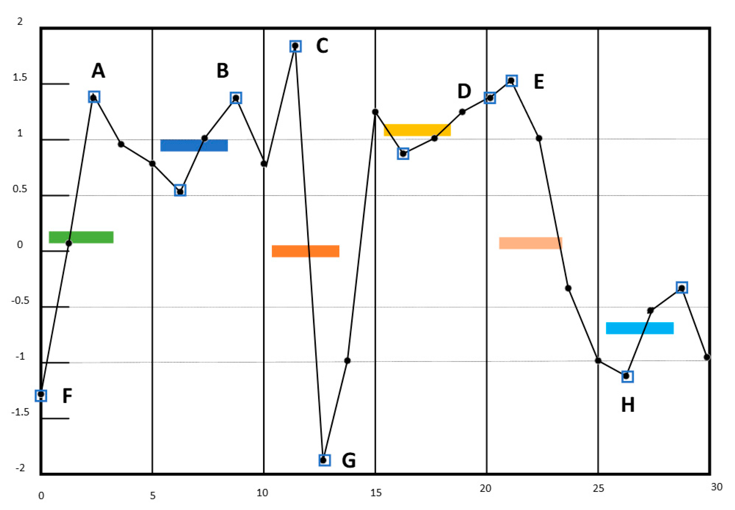
3.2. Our Method SAX-BD
3.3. Difference from ESAX
3.4. Lower Bound
4. Experimental Validation
4.1. Data Sets
4.2. Comparison Methods and Parameter Settings
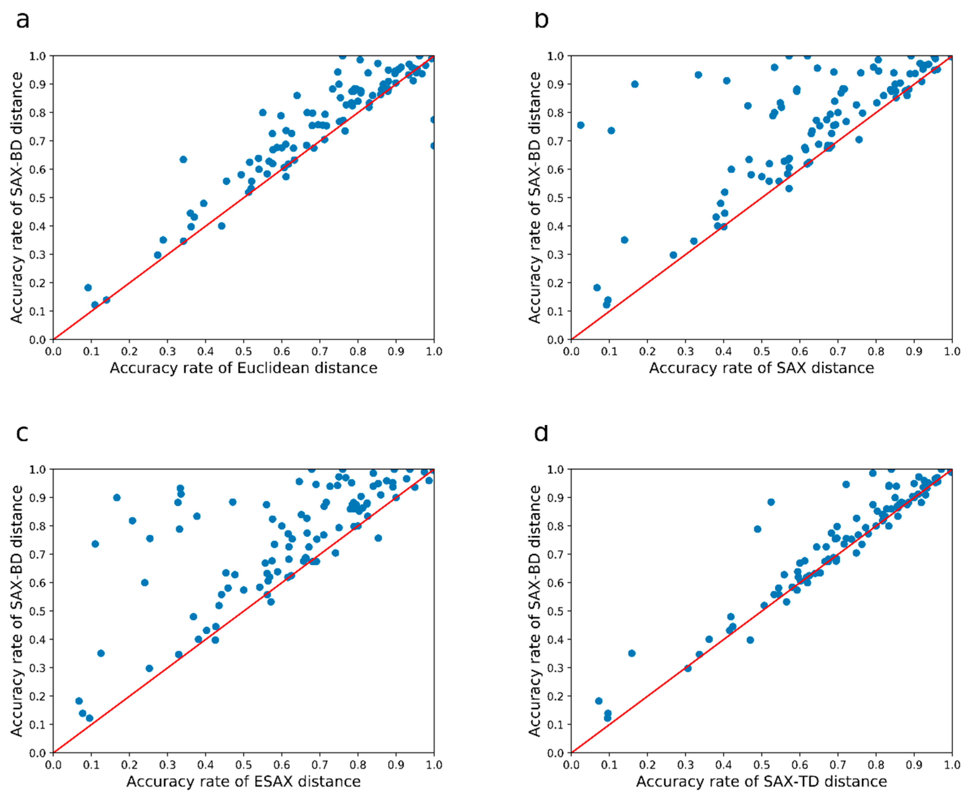
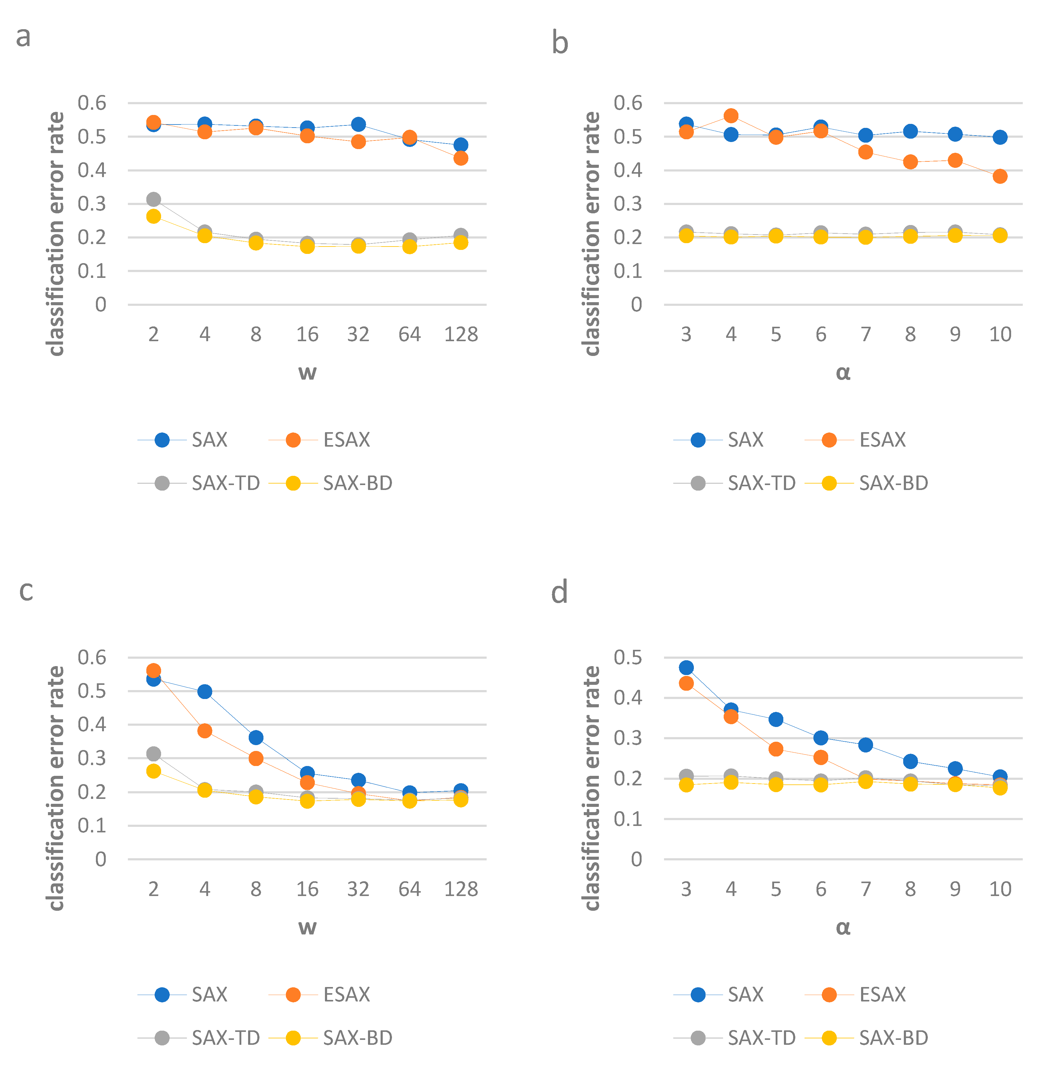
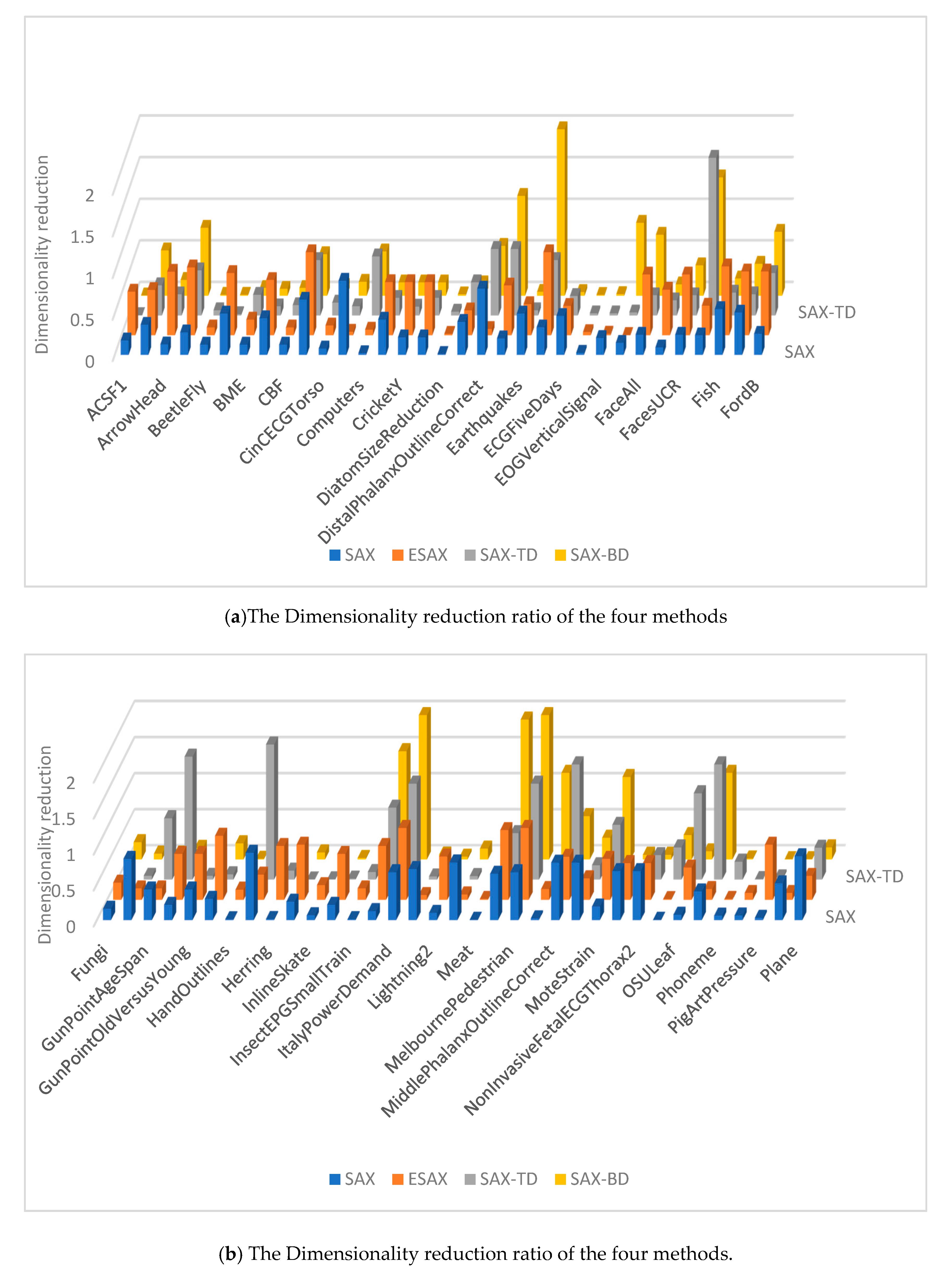
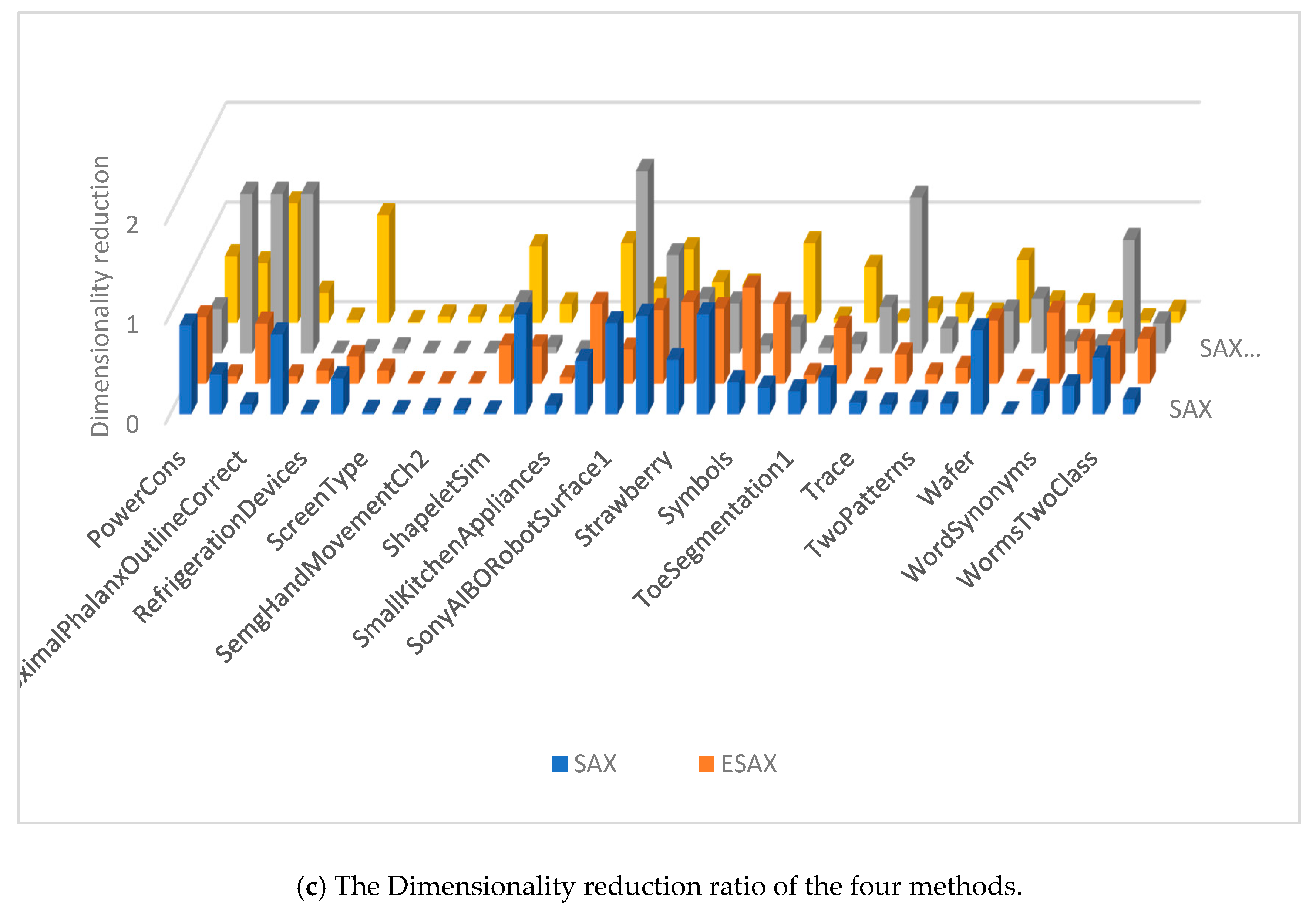
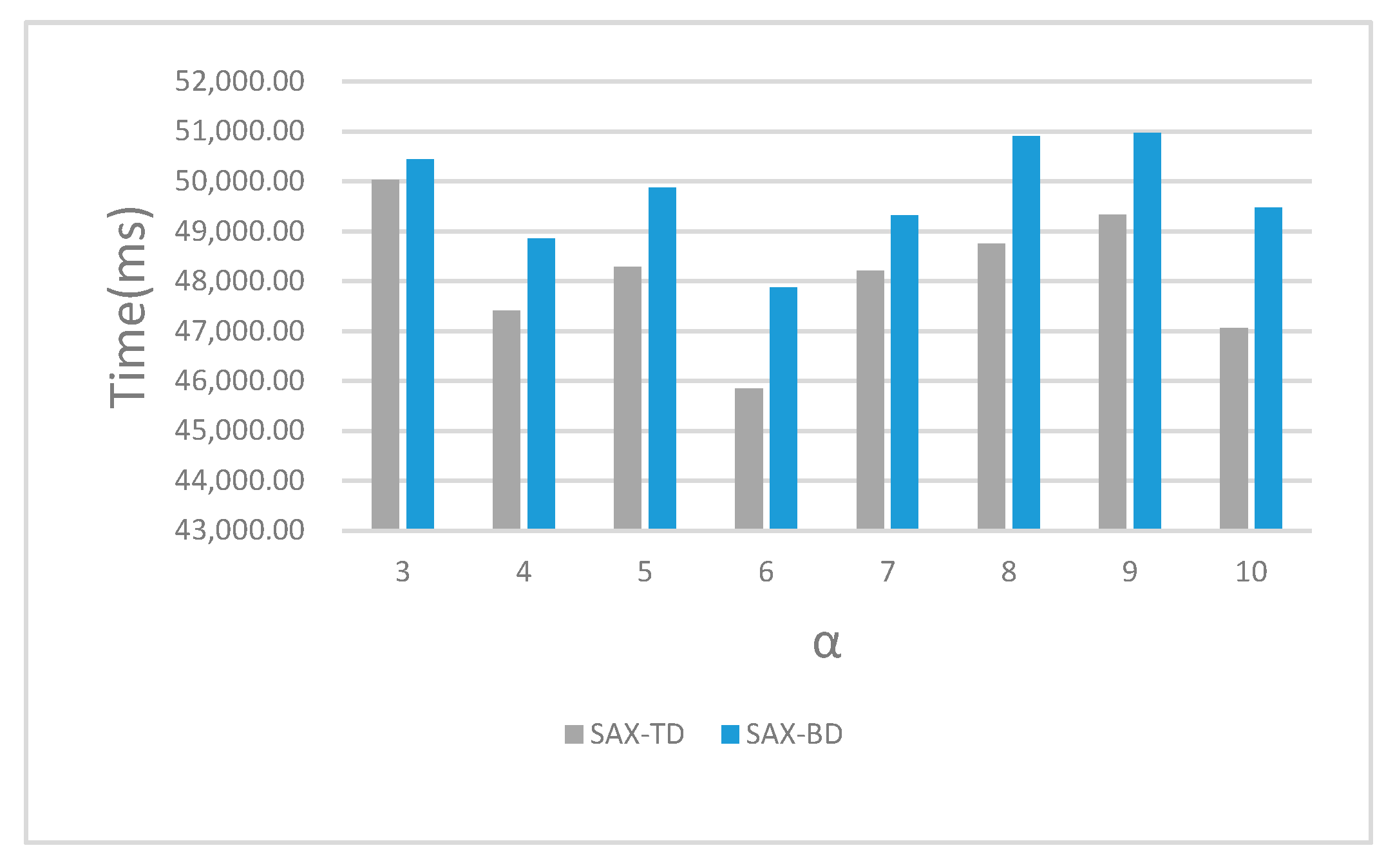
4.3. Result Analysis
5. Conclusions
Author Contributions
Funding
Conflicts of Interest
References
- Abanda, A.; Mori, U.; Lozano, J.A. A review on distance based time series classification. Data Min. Knowl. Discov. 2018, 33, 378–412. [Google Scholar] [CrossRef]
- Keogh, E.J.; Kasetty, S. On the Need for Time Series Data Mining Benchmarks: A Survey and Empirical Demonstration. Data Min. Knowl. Discov. 2003, 7, 349–371. [Google Scholar] [CrossRef]
- Vlachos, M.; Kollios, G.; Gunopulos, D. Discovering similar multidimensional trajectories. In Proceedings of the 18th International Conference on Data Engineering, San Jose, CA, USA, 26 Febuary–1 March 2002; p. 673. [Google Scholar]
- Lonardi, J.; Patel, P. Finding motifs in time series. In Proceedings of the 2nd Workshop on Temporal Data Mining, Washington, DC, USA, 24–27 August 2002. [Google Scholar]
- Keogh, E.; Lonardi, S.; Chiu, B.Y. Finding surprising patterns in a time series database in linear time and space. In Proceedings of the Eighth ACM SIGKDD International Conference on Knowledge Discovery and Data Mining, Edmonton, AB, Canada, 23–25 July 2002. [Google Scholar]
- Kalpakis, K.; Gada, D.; Puttagunta, V. Distance measures for effective clustering of ARIMA time-series. In Proceedings of the 2001 IEEE International Conference on Data Mining, San Jose, CA, USA, 29 November–2 December 2001; pp. 273–280. [Google Scholar]
- Huang, Y.-W.; Yu, P.S. Adaptive query processing for time-series data. In Proceedings of the Fifth ACM SIGKDD International Conference on Knowledge Discovery and Data Mining—KDD ’99, San Diego, CA, USA, 15–18 August 1999; pp. 282–286. [Google Scholar]
- Chan, K.-P.; Fu, A.W.-C. Efficient time series matching by wavelets. In Proceedings of the 15th International Conference on Data Engineering (Cat. No.99CB36337), Sydney, Australia, 23–26 March 1999; pp. 126–133. [Google Scholar]
- Dasgupta, D.; Forrest, S. Novelty detection in time series data using ideas from immunology. In Proceedings of the International Conference on Intelligent Systems, Ahmedabad, Indian, 15–16 November 1996. [Google Scholar]
- Xing, Z.; Pei, J.; Keogh, E. A brief survey on sequence classification. ACM SIGKDD Explor. Newsl. 2010, 12, 40–48. [Google Scholar] [CrossRef]
- Faloutsos, C.; Ranganathan, M.; Manolopoulos, Y. Fast subsequence matching in time-series databases. ACM Sigmod Rec. 1994, 23, 419–429. [Google Scholar] [CrossRef]
- Popivanov, I.; Miller, R. Similarity search over time-series data using wavelets. In Proceedings of the 18th International Conference on Data Engineering, Washington, DC, USA, 26 February–1 March 2002. [Google Scholar]
- Korn, F.; Jagadish, H.V.; Faloutsos, C. Efficiently supporting ad hoc queries in large datasets of time sequences. ACM Sigmod Rec. 1997, 26, 289–300. [Google Scholar] [CrossRef]
- Bagnall, A.; Janacek, G. A Run Length Transformation for Discriminating Between Auto Regressive Time Series. J. Classif. 2013, 31, 154–178. [Google Scholar] [CrossRef][Green Version]
- Corduas, M.; Piccolo, D. Time series clustering and classification by the autoregressive metric. Comput. Stat. Data Anal. 2008, 52, 1860–1872. [Google Scholar] [CrossRef]
- Smyth, P. Clustering sequences with hidden Markov models. In Proceedings of the Advances in Neural Information Processing Systems, Curitiba, Brazil, 2–5 November 1997. [Google Scholar]
- Berndt, D.J.; Clifford, J. Using dynamic time warping to find patterns in time series. In Proceedings of the KDD Workshop, Seattle, WA, USA, 31 July 1994. [Google Scholar]
- Keogh, E.J.; Chakrabarti, K.; Pazzani, M.J.; Mehrotra, S. Dimensionality Reduction for Fast Similarity Search in Large Time Series Databases. Knowl. Inf. Syst. 2001, 3, 263–286. [Google Scholar] [CrossRef]
- Hellerstein, J.M.; Koutsoupias, E.; Papadimitriou, C.H. On the analysis of indexing schemes. In Proceedings of the Sixteenth ACM SIGACT-SIGMOD-SIGART Symposium on Principles of Database Systems—PODS ’97, Tucson, AZ, USA, 12–14 May 1997. [Google Scholar]
- Lin, J.; Keogh, E.; Lonardi, S.; Chiu, B. A symbolic representation of time series, with implications for streaming algorithms. In Proceedings of the 8th ACM SIGMOD Workshop on Research Issues in Data Mining and Knowledge Discovery, San Diego, CA, USA, 13 June 2003. [Google Scholar]
- Tayebi, H.; Krishnaswamy, S.; Waluyo, A.B.; Sinha, A.; Abouelhoda, M.; Waluyo, A.B.; Sinha, A. RA-SAX: Resource-Aware Symbolic Aggregate Approximation for Mobile ECG Analysis. In Proceedings of the 2011 IEEE 12th International Conference on Mobile Data Management, Lulea, Sweden, 6–9 June 2011; Volume 1, pp. 289–290. [Google Scholar]
- Canelas, A.; Neves, R.F.; Horta, N. A new SAX-GA methodology applied to investment strategies optimization. In Proceedings of the Fourteenth International Conference on Genetic and Evolutionary Computation Conference Companion—GECCO Companion ’12, Philadelphia, PA, USA, 7–11 July 2012; pp. 1055–1062. [Google Scholar]
- Rakthanmanon, T.; Keogh, E. Fast shapelets: A scalable algorithm for discovering time series shapelets. In Proceedings of the 2013 SIAM International Conference on Data Mining, Austin, TX, USA, 2–4 May 2013. [Google Scholar]
- Zheng, Y.; Liu, Q.; Chen, E.; Ge, Y.; Zhao, J.L. Time Series Classification Using Multi-Channels Deep Convolutional Neural Networks. In Proceedings of the Lecture Notes in Computer Science, Leipzig, Germany, 22–26 June 2014; Springer Science and Business Media LLC: Macau, China, 2014; pp. 298–310. [Google Scholar]
- Lkhagva, B.; Suzuki, Y.; Kawagoe, K. New Time Series Data Representation ESAX for Financial Applications. In Proceedings of the 22nd International Conference on Data Engineering Workshops (ICDEW’06), Atlanta, GA, USA, 3–7 April 2006; p. 115. [Google Scholar]
- Sun, Y.; Li, J.; Liu, J.; Sun, B.; Chow, C. An improvement of symbolic aggregate approximation distance measure for time series. Neurocomputing 2014, 138, 189–198. [Google Scholar] [CrossRef]
- Dau, H.A.; Bagnall, A.; Kamgar, K.; Yeh, C.-C.M.; Zhu, Y.; Gharghabi, S.; Ratanamahatana, C.A.; Keogh, E. The UCR time series archive. IEEE/CAA J. Autom. Sin. 2019, 6, 1293–1305. [Google Scholar] [CrossRef]
- Lin, J.; Keogh, E.; Wei, L.; Lonardi, S. Experiencing SAX: A novel symbolic representation of time series. Data Min. Knowl. Discov. 2007, 15, 107–144. [Google Scholar] [CrossRef]


| 3 | 2 | 5 | 6 | 7 | 8 | 9 | 10 | |
|---|---|---|---|---|---|---|---|---|
| −0.43 | −0.67 | −0.84 | −0.97 | −1.07 | −1.15 | −1.22 | −1.28 | |
| −0.43 | 0 | −0.25 | −0.43 | −0.57 | −0.67 | −0.76 | −0.84 | |
| 0.67 | 0.25 | 0 | −0.18 | −0.32 | −0.43 | −0.52 | ||
| 0.84 | 0.43 | 0.18 | 0 | −0.14 | −0.25 | |||
| 0.97 | 0.57 | 0.32 | 0.14 | 0 | ||||
| 1.07 | 0.67 | 0.43 | 0.25 | |||||
| 1.15 | 0.76 | 0.52 | ||||||
| 1.22 | 0.84 | |||||||
| 1.28 |
| ID | Type | Name | Train | Test | Class | Length |
|---|---|---|---|---|---|---|
| 1 | Device | ACSF1 | 100 | 100 | 10 | 1460 |
| 2 | Image | Adiac | 390 | 391 | 37 | 176 |
| 3 | Image | ArrowHead | 36 | 175 | 3 | 251 |
| 4 | Spectro | Beef | 30 | 30 | 5 | 470 |
| 5 | Image | BeetleFly | 20 | 20 | 2 | 512 |
| 6 | Image | BirdChicken | 20 | 20 | 2 | 512 |
| 7 | Simulated | BME | 30 | 150 | 3 | 128 |
| 8 | Sensor | Car | 60 | 60 | 4 | 577 |
| 9 | Simulated | CBF | 30 | 900 | 3 | 128 |
| 10 | Traffic | Chinatown | 20 | 343 | 2 | 24 |
| 11 | Sensor | CinCECGTorso | 40 | 1380 | 4 | 1639 |
| 12 | Spectro | Coffee | 28 | 28 | 2 | 286 |
| 13 | Device | Computers | 250 | 250 | 2 | 720 |
| 14 | Motion | CricketX | 390 | 390 | 12 | 300 |
| 15 | Motion | CricketY | 390 | 390 | 12 | 300 |
| 16 | Motion | CricketZ | 390 | 390 | 12 | 300 |
| 17 | Image | DiatomSizeReduction | 16 | 306 | 4 | 345 |
| 18 | Image | DistalPhalanxOutlineAgeGroup | 400 | 139 | 3 | 80 |
| 19 | Image | DistalPhalanxOutlineCorrect | 600 | 276 | 2 | 80 |
| 20 | Image | DistalPhalanxTW | 400 | 139 | 6 | 80 |
| 21 | Sensor | Earthquakes | 322 | 139 | 2 | 512 |
| 22 | ECG | ECG200 | 100 | 100 | 2 | 96 |
| 23 | ECG | ECGFiveDays | 23 | 861 | 2 | 136 |
| 24 | EOG | EOGHorizontalSignal | 362 | 362 | 12 | 1250 |
| 25 | EOG | EOGVerticalSignal | 362 | 362 | 12 | 1250 |
| 26 | Spectro | EthanolLevel | 504 | 500 | 4 | 1751 |
| 27 | Image | FaceAll | 560 | 1690 | 14 | 131 |
| 28 | Image | FaceFour | 24 | 88 | 4 | 350 |
| 29 | Image | FacesUCR | 200 | 2050 | 14 | 131 |
| 30 | Image | FiftyWords | 450 | 455 | 50 | 270 |
| 31 | Image | Fish | 175 | 175 | 7 | 463 |
| 32 | Sensor | FordA | 3601 | 1320 | 2 | 500 |
| 33 | Sensor | FordB | 3636 | 810 | 2 | 500 |
| 34 | HRM | Fungi | 18 | 186 | 18 | 201 |
| 35 | Motion | GunPoint | 50 | 150 | 2 | 150 |
| 36 | Motion | GunPointAgeSpan | 135 | 316 | 2 | 150 |
| 37 | Motion | GunPointMaleVersusFemale | 135 | 316 | 2 | 150 |
| 38 | Motion | GunPointOldVersusYoung | 136 | 315 | 2 | 150 |
| 39 | Spectro | Ham | 109 | 105 | 2 | 431 |
| 40 | Image | HandOutlines | 1000 | 370 | 2 | 2709 |
| 41 | Motion | Haptics | 155 | 308 | 5 | 1092 |
| 42 | Image | Herring | 64 | 64 | 2 | 512 |
| 43 | Device | HouseTwenty | 40 | 119 | 2 | 2000 |
| 44 | Motion | InlineSkate | 100 | 550 | 7 | 1882 |
| 45 | EPG | InsectEPGRegularTrain | 62 | 249 | 3 | 601 |
| 46 | EPG | InsectEPGSmallTrain | 17 | 249 | 3 | 601 |
| 47 | Sensor | InsectWingbeatSound | 220 | 1980 | 11 | 256 |
| 48 | Sensor | ItalyPowerDemand | 67 | 1029 | 2 | 24 |
| 49 | Device | LargeKitchenAppliances | 375 | 375 | 3 | 720 |
| 50 | Sensor | Lightning2 | 60 | 61 | 2 | 637 |
| 51 | Sensor | Lightning7 | 70 | 73 | 7 | 319 |
| 52 | Spectro | Meat | 60 | 60 | 3 | 448 |
| 53 | Image | MedicalImages | 381 | 760 | 10 | 99 |
| 54 | Traffic | MelbournePedestrian | 1194 | 2439 | 10 | 24 |
| 55 | Image | MiddlePhalanxOutlineAgeGroup | 400 | 154 | 3 | 80 |
| 56 | Image | MiddlePhalanxOutlineCorrect | 600 | 291 | 2 | 80 |
| 57 | Image | MiddlePhalanxTW | 399 | 154 | 6 | 80 |
| 58 | Sensor | MoteStrain | 20 | 1252 | 2 | 84 |
| 59 | ECG | NonInvasiveFetalECGThorax1 | 1800 | 1965 | 42 | 750 |
| 60 | ECG | NonInvasiveFetalECGThorax2 | 1800 | 1965 | 42 | 750 |
| 61 | Spectro | OliveOil | 30 | 30 | 4 | 570 |
| 62 | Image | OSULeaf | 200 | 242 | 6 | 427 |
| 63 | Image | PhalangesOutlinesCorrect | 1800 | 858 | 2 | 80 |
| 64 | Sensor | Phoneme | 214 | 1896 | 39 | 1024 |
| 65 | Hemodynamics | PigAirwayPressure | 104 | 208 | 52 | 2000 |
| 66 | Hemodynamics | PigArtPressure | 104 | 208 | 52 | 2000 |
| 67 | Hemodynamics | PigCVP | 104 | 208 | 52 | 2000 |
| 68 | Sensor | Plane | 105 | 105 | 7 | 144 |
| 69 | Power | PowerCons | 180 | 180 | 2 | 144 |
| 70 | Image | ProximalPhalanxOutlineAgeGroup | 400 | 205 | 3 | 80 |
| 71 | Image | ProximalPhalanxOutlineCorrect | 600 | 291 | 2 | 80 |
| 72 | Image | ProximalPhalanxTW | 400 | 205 | 6 | 80 |
| 73 | Device | RefrigerationDevices | 375 | 375 | 3 | 720 |
| 74 | Spectrum | Rock | 20 | 50 | 4 | 2844 |
| 75 | Device | ScreenType | 375 | 375 | 3 | 720 |
| 76 | Spectrum | SemgHandGenderCh2 | 300 | 600 | 2 | 1500 |
| 77 | Spectrum | SemgHandMovementCh2 | 450 | 450 | 6 | 1500 |
| 78 | Spectrum | SemgHandSubjectCh2 | 450 | 450 | 5 | 1500 |
| 79 | Simulated | ShapeletSim | 20 | 180 | 2 | 500 |
| 80 | Image | ShapesAll | 600 | 600 | 60 | 512 |
| 81 | Device | SmallKitchenAppliances | 375 | 375 | 3 | 720 |
| 82 | Simulated | SmoothSubspace | 150 | 150 | 3 | 15 |
| 83 | Sensor | SonyAIBORobotSurface1 | 20 | 601 | 2 | 70 |
| 84 | Sensor | SonyAIBORobotSurface2 | 27 | 953 | 2 | 65 |
| 85 | Spectro | Strawberry | 613 | 370 | 2 | 235 |
| 86 | Image | SwedishLeaf | 500 | 625 | 15 | 128 |
| 87 | Image | Symbols | 25 | 995 | 6 | 398 |
| 88 | Simulated | SyntheticControl | 300 | 300 | 6 | 60 |
| 89 | Motion | ToeSegmentation1 | 40 | 228 | 2 | 277 |
| 90 | Motion | ToeSegmentation2 | 36 | 130 | 2 | 343 |
| 91 | Sensor | Trace | 100 | 100 | 4 | 275 |
| 92 | ECG | TwoLeadECG | 23 | 1139 | 2 | 82 |
| 93 | Simulated | TwoPatterns | 1000 | 4000 | 4 | 128 |
| 94 | Simulated | UMD | 36 | 144 | 3 | 150 |
| 95 | Sensor | Wafer | 1000 | 6164 | 2 | 152 |
| 96 | Spectro | Wine | 57 | 54 | 2 | 234 |
| 97 | Image | WordSynonyms | 267 | 638 | 25 | 270 |
| 98 | Motion | Worms | 181 | 77 | 5 | 900 |
| 99 | Motion | WormsTwoClass | 181 | 77 | 2 | 900 |
| 100 | Image | Yoga | 300 | 3000 | 2 | 426 |
| ID | EU Error | SAX Error | SAX w | SAX Ratio | SAX α | ESAX Error | ESAX w | ESAX Ratio | ESAX α | SAXTD Error | SAXTD w | SAXTD Ratio | SAXTD α | SAXBD Error | SAXBD w | SAXBD Ratio | SAXBD α |
|---|---|---|---|---|---|---|---|---|---|---|---|---|---|---|---|---|---|
| 1 | 0.460 | 0.580 | 256 | 0.175 | 8 | 0.760 | 256 | 0.526 | 3 | 0.380 | 4 | 0.005 | 3 | 0.400 | 2 | 0.004 | 3 |
| 2 | 0.389 | 0.895 | 64 | 0.364 | 9 | 0.890 | 32 | 0.545 | 7 | 0.284 | 32 | 0.364 | 3 | 0.263 | 32 | 0.545 | 4 |
| 3 | 0.200 | 0.309 | 32 | 0.127 | 10 | 0.349 | 64 | 0.765 | 10 | 0.183 | 32 | 0.255 | 3 | 0.160 | 16 | 0.191 | 5 |
| 4 | 0.333 | 0.467 | 128 | 0.272 | 7 | 0.400 | 128 | 0.817 | 7 | 0.167 | 128 | 0.545 | 4 | 0.200 | 128 | 0.817 | 6 |
| 5 | 0.250 | 0.150 | 64 | 0.125 | 4 | 0.100 | 16 | 0.094 | 4 | 0.150 | 16 | 0.063 | 5 | 0.100 | 2 | 0.012 | 3 |
| 6 | 0.450 | 0.300 | 256 | 0.500 | 4 | 0.200 | 128 | 0.750 | 5 | 0.200 | 4 | 0.016 | 4 | 0.200 | 2 | 0.012 | 3 |
| 7 | 0.173 | 0.153 | 16 | 0.125 | 7 | 0.160 | 8 | 0.188 | 7 | 0.147 | 16 | 0.250 | 3 | 0.060 | 4 | 0.094 | 4 |
| 8 | 0.267 | 0.283 | 256 | 0.444 | 10 | 0.283 | 128 | 0.666 | 6 | 0.133 | 32 | 0.111 | 4 | 0.117 | 16 | 0.083 | 3 |
| 9 | 0.148 | 0.084 | 16 | 0.125 | 8 | 0.250 | 4 | 0.094 | 9 | 0.088 | 8 | 0.125 | 5 | 0.027 | 4 | 0.094 | 4 |
| 10 | 0.058 | 0.467 | 16 | 0.667 | 7 | 0.125 | 8 | 1.000 | 7 | 0.041 | 8 | 0.667 | 3 | 0.041 | 4 | 0.500 | 3 |
| 11 | 0.103 | 0.097 | 128 | 0.078 | 9 | 0.108 | 64 | 0.117 | 10 | 0.072 | 128 | 0.156 | 9 | 0.062 | 64 | 0.117 | 8 |
| 12 | 0.000 | 0.429 | 256 | 0.895 | 4 | 0.321 | 4 | 0.042 | 6 | 0.000 | 16 | 0.112 | 3 | 0.000 | 16 | 0.168 | 3 |
| 13 | 0.424 | 0.480 | 16 | 0.022 | 6 | 0.432 | 16 | 0.067 | 4 | 0.404 | 256 | 0.711 | 3 | 0.380 | 128 | 0.533 | 3 |
| 14 | 0.423 | 0.385 | 128 | 0.427 | 9 | 0.444 | 64 | 0.640 | 10 | 0.400 | 32 | 0.213 | 6 | 0.331 | 16 | 0.160 | 5 |
| 15 | 0.433 | 0.441 | 64 | 0.213 | 8 | 0.523 | 64 | 0.640 | 8 | 0.441 | 16 | 0.107 | 7 | 0.372 | 16 | 0.160 | 6 |
| 16 | 0.413 | 0.387 | 64 | 0.213 | 10 | 0.426 | 64 | 0.640 | 10 | 0.387 | 32 | 0.213 | 6 | 0.323 | 16 | 0.160 | 7 |
| 17 | 0.065 | 0.062 | 4 | 0.012 | 6 | 0.232 | 2 | 0.017 | 4 | 0.039 | 8 | 0.046 | 4 | 0.029 | 2 | 0.017 | 3 |
| 18 | 0.374 | 0.317 | 32 | 0.400 | 4 | 0.381 | 8 | 0.300 | 4 | 0.331 | 16 | 0.400 | 4 | 0.273 | 4 | 0.150 | 3 |
| 19 | 0.283 | 0.348 | 64 | 0.800 | 6 | 0.308 | 2 | 0.075 | 8 | 0.264 | 32 | 0.800 | 4 | 0.246 | 16 | 0.600 | 4 |
| 20 | 0.367 | 0.432 | 16 | 0.200 | 6 | 0.439 | 16 | 0.600 | 9 | 0.360 | 32 | 0.800 | 4 | 0.367 | 32 | 1.200 | 5 |
| 21 | 0.288 | 0.245 | 256 | 0.500 | 6 | 0.259 | 64 | 0.375 | 5 | 0.252 | 16 | 0.063 | 3 | 0.295 | 8 | 0.047 | 3 |
| 22 | 0.120 | 0.080 | 32 | 0.333 | 6 | 0.140 | 32 | 1.000 | 5 | 0.070 | 32 | 0.667 | 4 | 0.090 | 64 | 2.000 | 5 |
| 23 | 0.203 | 0.114 | 64 | 0.471 | 8 | 0.211 | 16 | 0.353 | 8 | 0.081 | 16 | 0.235 | 4 | 0.117 | 2 | 0.044 | 3 |
| 24 | 0.558 | 0.616 | 32 | 0.026 | 9 | 0.619 | 16 | 0.038 | 8 | 0.638 | 16 | 0.026 | 4 | 0.599 | 4 | 0.010 | 6 |
| 25 | 0.638 | 0.599 | 256 | 0.205 | 9 | 0.575 | 8 | 0.019 | 8 | 0.530 | 16 | 0.026 | 4 | 0.602 | 8 | 0.019 | 6 |
| 26 | 0.726 | 0.732 | 256 | 0.146 | 5 | 0.748 | 2 | 0.003 | 3 | 0.694 | 32 | 0.037 | 4 | 0.702 | 512 | 0.877 | 4 |
| 27 | 0.286 | 0.320 | 32 | 0.244 | 9 | 0.250 | 32 | 0.733 | 8 | 0.227 | 16 | 0.244 | 5 | 0.206 | 32 | 0.733 | 3 |
| 28 | 0.216 | 0.159 | 32 | 0.091 | 8 | 0.205 | 64 | 0.549 | 9 | 0.136 | 32 | 0.183 | 5 | 0.125 | 16 | 0.137 | 3 |
| 29 | 0.231 | 0.252 | 32 | 0.244 | 10 | 0.334 | 32 | 0.733 | 10 | 0.251 | 16 | 0.244 | 9 | 0.173 | 16 | 0.366 | 5 |
| 30 | 0.369 | 0.327 | 64 | 0.237 | 9 | 0.319 | 32 | 0.356 | 8 | 0.334 | 256 | 1.896 | 7 | 0.325 | 128 | 1.422 | 5 |
| 31 | 0.217 | 0.451 | 256 | 0.553 | 8 | 0.623 | 128 | 0.829 | 8 | 0.143 | 64 | 0.276 | 4 | 0.166 | 32 | 0.207 | 5 |
| 32 | 0.335 | 0.327 | 256 | 0.512 | 7 | 0.336 | 128 | 0.768 | 8 | 0.304 | 64 | 0.256 | 3 | 0.315 | 64 | 0.384 | 3 |
| 33 | 0.394 | 0.428 | 128 | 0.256 | 6 | 0.436 | 128 | 0.768 | 6 | 0.399 | 128 | 0.512 | 5 | 0.394 | 128 | 0.768 | 5 |
| 34 | 0.161 | 0.118 | 32 | 0.159 | 6 | 0.210 | 16 | 0.239 | 7 | 0.172 | 16 | 0.159 | 3 | 0.140 | 16 | 0.239 | 3 |
| 35 | 0.087 | 0.207 | 128 | 0.853 | 5 | 0.013 | 8 | 0.160 | 6 | 0.073 | 4 | 0.053 | 5 | 0.040 | 4 | 0.080 | 5 |
| 36 | 0.032 | 0.111 | 64 | 0.427 | 8 | 0.051 | 8 | 0.160 | 7 | 0.076 | 64 | 0.853 | 3 | 0.063 | 4 | 0.080 | 4 |
| 37 | 0.006 | 0.044 | 32 | 0.213 | 9 | 0.025 | 32 | 0.640 | 9 | 0.003 | 128 | 1.707 | 3 | 0.009 | 8 | 0.160 | 3 |
| 38 | 0.000 | 0.108 | 64 | 0.427 | 9 | 0.063 | 32 | 0.640 | 9 | 0.000 | 4 | 0.053 | 3 | 0.000 | 2 | 0.040 | 3 |
| 39 | 0.400 | 0.324 | 128 | 0.297 | 7 | 0.343 | 128 | 0.891 | 6 | 0.305 | 16 | 0.074 | 4 | 0.324 | 32 | 0.223 | 4 |
| 40 | 0.138 | 0.162 | 32 | 0.012 | 7 | 0.176 | 128 | 0.142 | 8 | 0.130 | 8 | 0.006 | 4 | 0.119 | 8 | 0.009 | 3 |
| 41 | 0.630 | 0.620 | 1024 | 0.938 | 6 | 0.597 | 128 | 0.352 | 7 | 0.584 | 1024 | 1.875 | 7 | 0.568 | 32 | 0.088 | 3 |
| 42 | 0.484 | 0.375 | 8 | 0.016 | 5 | 0.375 | 128 | 0.750 | 5 | 0.375 | 32 | 0.125 | 3 | 0.375 | 16 | 0.094 | 4 |
| 43 | 0.319 | 0.235 | 512 | 0.256 | 7 | 0.210 | 512 | 0.768 | 7 | 0.303 | 2 | 0.002 | 3 | 0.202 | 64 | 0.096 | 3 |
| 44 | 0.658 | 0.678 | 128 | 0.068 | 10 | 0.671 | 128 | 0.204 | 9 | 0.664 | 4 | 0.004 | 4 | 0.653 | 4 | 0.006 | 7 |
| 45 | 0.000 | 0.329 | 128 | 0.213 | 5 | 0.333 | 128 | 0.639 | 6 | 0.317 | 4 | 0.013 | 5 | 0.225 | 4 | 0.020 | 4 |
| 46 | 0.000 | 0.317 | 8 | 0.013 | 8 | 0.382 | 32 | 0.160 | 5 | 0.325 | 32 | 0.106 | 4 | 0.317 | 32 | 0.160 | 4 |
| 47 | 0.438 | 0.432 | 32 | 0.125 | 8 | 0.458 | 64 | 0.750 | 7 | 0.420 | 128 | 1.000 | 5 | 0.416 | 128 | 1.500 | 4 |
| 48 | 0.045 | 0.077 | 16 | 0.667 | 9 | 0.109 | 8 | 1.000 | 8 | 0.044 | 16 | 1.333 | 3 | 0.047 | 16 | 2.000 | 4 |
| 49 | 0.507 | 0.528 | 512 | 0.711 | 8 | 0.541 | 16 | 0.067 | 8 | 0.456 | 16 | 0.044 | 4 | 0.419 | 16 | 0.067 | 4 |
| 50 | 0.246 | 0.148 | 64 | 0.100 | 7 | 0.197 | 128 | 0.603 | 5 | 0.197 | 16 | 0.050 | 6 | 0.148 | 8 | 0.038 | 4 |
| 51 | 0.425 | 0.370 | 256 | 0.803 | 6 | 0.329 | 8 | 0.075 | 6 | 0.356 | 8 | 0.050 | 6 | 0.274 | 16 | 0.150 | 4 |
| 52 | 0.067 | 0.667 | 2 | 0.004 | 3 | 0.667 | 2 | 0.013 | 3 | 0.067 | 16 | 0.071 | 3 | 0.067 | 2 | 0.013 | 3 |
| 53 | 0.316 | 0.322 | 64 | 0.646 | 7 | 0.309 | 32 | 0.970 | 9 | 0.325 | 32 | 0.646 | 5 | 0.325 | 64 | 1.939 | 6 |
| 54 | 0.055 | 0.592 | 16 | 0.667 | 10 | 0.665 | 8 | 1.000 | 9 | 0.089 | 16 | 1.333 | 3 | 0.087 | 16 | 2.000 | 3 |
| 55 | 0.481 | 0.429 | 2 | 0.025 | 3 | 0.429 | 4 | 0.150 | 3 | 0.435 | 2 | 0.050 | 3 | 0.468 | 32 | 1.200 | 3 |
| 56 | 0.234 | 0.368 | 64 | 0.800 | 8 | 0.419 | 16 | 0.600 | 4 | 0.237 | 64 | 1.600 | 5 | 0.265 | 16 | 0.600 | 5 |
| 57 | 0.487 | 0.597 | 64 | 0.800 | 6 | 0.565 | 8 | 0.300 | 7 | 0.494 | 8 | 0.200 | 3 | 0.481 | 8 | 0.300 | 3 |
| 58 | 0.121 | 0.149 | 16 | 0.190 | 5 | 0.215 | 16 | 0.571 | 6 | 0.118 | 32 | 0.762 | 5 | 0.125 | 32 | 1.143 | 6 |
| 59 | 0.171 | 0.448 | 512 | 0.683 | 10 | 0.792 | 128 | 0.512 | 10 | 0.183 | 32 | 0.085 | 4 | 0.181 | 16 | 0.064 | 5 |
| 60 | 0.120 | 0.408 | 512 | 0.683 | 10 | 0.673 | 128 | 0.512 | 10 | 0.115 | 128 | 0.341 | 5 | 0.117 | 16 | 0.064 | 8 |
| 61 | 0.133 | 0.833 | 2 | 0.004 | 3 | 0.833 | 2 | 0.011 | 3 | 0.100 | 128 | 0.449 | 3 | 0.100 | 64 | 0.337 | 3 |
| 62 | 0.479 | 0.455 | 32 | 0.075 | 6 | 0.438 | 64 | 0.450 | 8 | 0.455 | 256 | 1.199 | 5 | 0.442 | 16 | 0.112 | 3 |
| 63 | 0.239 | 0.357 | 32 | 0.400 | 5 | 0.383 | 4 | 0.150 | 3 | 0.220 | 64 | 1.600 | 4 | 0.227 | 32 | 1.200 | 4 |
| 64 | 0.891 | 0.908 | 64 | 0.063 | 8 | 0.905 | 4 | 0.012 | 6 | 0.905 | 128 | 0.250 | 8 | 0.878 | 4 | 0.012 | 3 |
| 65 | 0.909 | 0.933 | 128 | 0.064 | 8 | 0.933 | 64 | 0.096 | 6 | 0.928 | 8 | 0.008 | 3 | 0.817 | 2 | 0.003 | 3 |
| 66 | 0.712 | 0.861 | 64 | 0.032 | 5 | 0.875 | 512 | 0.768 | 3 | 0.841 | 32 | 0.032 | 4 | 0.649 | 2 | 0.003 | 3 |
| 67 | 0.861 | 0.904 | 1024 | 0.512 | 5 | 0.923 | 64 | 0.096 | 4 | 0.904 | 64 | 0.064 | 3 | 0.861 | 2 | 0.003 | 3 |
| 68 | 0.038 | 0.048 | 128 | 0.889 | 9 | 0.105 | 16 | 0.333 | 8 | 0.029 | 32 | 0.444 | 3 | 0.000 | 8 | 0.167 | 3 |
| 69 | 0.022 | 0.072 | 128 | 0.889 | 6 | 0.072 | 32 | 0.667 | 6 | 0.044 | 32 | 0.444 | 5 | 0.033 | 32 | 0.667 | 6 |
| 70 | 0.215 | 0.537 | 32 | 0.400 | 6 | 0.424 | 2 | 0.075 | 6 | 0.180 | 64 | 1.600 | 3 | 0.176 | 16 | 0.600 | 3 |
| 71 | 0.192 | 0.292 | 8 | 0.100 | 6 | 0.289 | 16 | 0.600 | 4 | 0.144 | 64 | 1.600 | 3 | 0.131 | 32 | 1.200 | 3 |
| 72 | 0.293 | 0.976 | 64 | 0.800 | 4 | 0.746 | 2 | 0.075 | 7 | 0.278 | 64 | 1.600 | 3 | 0.244 | 8 | 0.300 | 3 |
| 73 | 0.605 | 0.608 | 16 | 0.022 | 5 | 0.632 | 32 | 0.133 | 5 | 0.581 | 2 | 0.006 | 3 | 0.520 | 8 | 0.033 | 3 |
| 74 | 0.360 | 0.180 | 1024 | 0.360 | 4 | 0.220 | 256 | 0.270 | 4 | 0.160 | 32 | 0.023 | 3 | 0.140 | 1024 | 1.080 | 4 |
| 75 | 0.640 | 0.597 | 16 | 0.022 | 6 | 0.573 | 32 | 0.133 | 8 | 0.576 | 16 | 0.044 | 3 | 0.555 | 2 | 0.008 | 3 |
| 76 | 0.102 | 0.193 | 32 | 0.021 | 8 | 0.310 | 4 | 0.008 | 7 | 0.278 | 4 | 0.005 | 5 | 0.053 | 32 | 0.064 | 5 |
| 77 | 0.402 | 0.471 | 64 | 0.043 | 9 | 0.669 | 4 | 0.008 | 10 | 0.511 | 4 | 0.005 | 7 | 0.211 | 32 | 0.064 | 7 |
| 78 | 0.209 | 0.287 | 64 | 0.043 | 9 | 0.529 | 4 | 0.008 | 9 | 0.476 | 4 | 0.005 | 6 | 0.116 | 32 | 0.064 | 5 |
| 79 | 0.461 | 0.428 | 8 | 0.016 | 4 | 0.411 | 64 | 0.384 | 5 | 0.406 | 128 | 0.512 | 6 | 0.361 | 128 | 0.768 | 4 |
| 80 | 0.248 | 0.278 | 512 | 1.000 | 10 | 0.290 | 64 | 0.375 | 9 | 0.247 | 16 | 0.063 | 4 | 0.232 | 32 | 0.188 | 3 |
| 81 | 0.659 | 0.533 | 64 | 0.089 | 7 | 0.547 | 16 | 0.067 | 5 | 0.347 | 4 | 0.011 | 6 | 0.365 | 4 | 0.017 | 6 |
| 82 | 0.047 | 0.240 | 8 | 0.533 | 8 | 0.273 | 4 | 0.800 | 7 | 0.167 | 2 | 0.267 | 3 | 0.060 | 4 | 0.800 | 3 |
| 83 | 0.304 | 0.306 | 64 | 0.914 | 6 | 0.146 | 8 | 0.343 | 4 | 0.303 | 64 | 1.829 | 4 | 0.243 | 8 | 0.343 | 3 |
| 84 | 0.141 | 0.120 | 64 | 0.985 | 6 | 0.188 | 16 | 0.738 | 5 | 0.143 | 32 | 0.985 | 5 | 0.136 | 16 | 0.738 | 10 |
| 85 | 0.054 | 0.354 | 128 | 0.545 | 4 | 0.354 | 64 | 0.817 | 4 | 0.038 | 64 | 0.545 | 3 | 0.043 | 32 | 0.409 | 3 |
| 86 | 0.211 | 0.408 | 128 | 1.000 | 10 | 0.440 | 32 | 0.750 | 10 | 0.208 | 32 | 0.500 | 4 | 0.125 | 16 | 0.375 | 5 |
| 87 | 0.101 | 0.137 | 128 | 0.322 | 9 | 0.192 | 128 | 0.965 | 8 | 0.104 | 16 | 0.080 | 5 | 0.095 | 8 | 0.060 | 7 |
| 88 | 0.120 | 0.047 | 16 | 0.267 | 8 | 0.147 | 16 | 0.800 | 8 | 0.100 | 8 | 0.267 | 8 | 0.050 | 16 | 0.800 | 8 |
| 89 | 0.320 | 0.311 | 64 | 0.231 | 6 | 0.373 | 8 | 0.087 | 5 | 0.307 | 8 | 0.058 | 4 | 0.246 | 4 | 0.043 | 3 |
| 90 | 0.192 | 0.123 | 128 | 0.373 | 7 | 0.177 | 64 | 0.560 | 4 | 0.138 | 16 | 0.093 | 5 | 0.123 | 64 | 0.560 | 5 |
| 91 | 0.240 | 0.380 | 32 | 0.116 | 6 | 0.240 | 4 | 0.044 | 7 | 0.160 | 64 | 0.465 | 3 | 0.000 | 2 | 0.022 | 3 |
| 92 | 0.253 | 0.311 | 8 | 0.098 | 7 | 0.254 | 8 | 0.293 | 7 | 0.166 | 64 | 1.561 | 4 | 0.057 | 4 | 0.146 | 3 |
| 93 | 0.093 | 0.039 | 16 | 0.125 | 9 | 0.217 | 4 | 0.094 | 10 | 0.063 | 16 | 0.250 | 8 | 0.048 | 8 | 0.188 | 6 |
| 94 | 0.194 | 0.194 | 16 | 0.107 | 9 | 0.160 | 8 | 0.160 | 6 | 0.208 | 16 | 0.213 | 4 | 0.014 | 4 | 0.080 | 3 |
| 95 | 0.005 | 0.002 | 128 | 0.842 | 6 | 0.002 | 32 | 0.632 | 7 | 0.003 | 32 | 0.421 | 5 | 0.003 | 32 | 0.632 | 7 |
| 96 | 0.389 | 0.500 | 2 | 0.009 | 3 | 0.500 | 2 | 0.026 | 3 | 0.407 | 64 | 0.547 | 3 | 0.426 | 16 | 0.205 | 3 |
| 97 | 0.382 | 0.381 | 64 | 0.237 | 8 | 0.384 | 64 | 0.711 | 10 | 0.382 | 16 | 0.119 | 7 | 0.381 | 16 | 0.178 | 4 |
| 98 | 0.545 | 0.481 | 256 | 0.284 | 4 | 0.558 | 128 | 0.427 | 4 | 0.468 | 32 | 0.071 | 4 | 0.442 | 32 | 0.107 | 4 |
| 99 | 0.390 | 0.351 | 512 | 0.569 | 4 | 0.338 | 128 | 0.427 | 5 | 0.312 | 512 | 1.138 | 4 | 0.312 | 8 | 0.027 | 4 |
| 100 | 0.170 | 0.198 | 64 | 0.150 | 10 | 0.174 | 64 | 0.451 | 10 | 0.176 | 64 | 0.300 | 6 | 0.166 | 16 | 0.113 | 5 |
| Methods | n* | n | n0 | p-Value |
|---|---|---|---|---|
| SAX-BD vs. Euclidean | 79 | 15 | 6 | p < 0.05 |
| SAX-BD vs. SAX | 83 | 11 | 6 | p < 0.05 |
| SAX-BD vs. ESAX | 87 | 10 | 3 | p < 0.05 |
| SAX-BD vs. SAX-TD | 69 | 22 | 10 | p < 0.05 |
Publisher’s Note: MDPI stays neutral with regard to jurisdictional claims in published maps and institutional affiliations. |
© 2020 by the authors. Licensee MDPI, Basel, Switzerland. This article is an open access article distributed under the terms and conditions of the Creative Commons Attribution (CC BY) license (http://creativecommons.org/licenses/by/4.0/).
Share and Cite
He, Z.; Long, S.; Ma, X.; Zhao, H. A Boundary Distance-Based Symbolic Aggregate Approximation Method for Time Series Data. Algorithms 2020, 13, 284. https://doi.org/10.3390/a13110284
He Z, Long S, Ma X, Zhao H. A Boundary Distance-Based Symbolic Aggregate Approximation Method for Time Series Data. Algorithms. 2020; 13(11):284. https://doi.org/10.3390/a13110284
Chicago/Turabian StyleHe, Zhenwen, Shirong Long, Xiaogang Ma, and Hong Zhao. 2020. "A Boundary Distance-Based Symbolic Aggregate Approximation Method for Time Series Data" Algorithms 13, no. 11: 284. https://doi.org/10.3390/a13110284
APA StyleHe, Z., Long, S., Ma, X., & Zhao, H. (2020). A Boundary Distance-Based Symbolic Aggregate Approximation Method for Time Series Data. Algorithms, 13(11), 284. https://doi.org/10.3390/a13110284