Differential Evolution with Linear Bias Reduction in Parameter Adaptation

Abstract

In this study, a new parameter control scheme is proposed for the differential evolution algorithm. The developed linear bias reduction scheme controls the Lehmer mean parameter value depending on the optimization stage, allowing the algorithm to improve the exploration properties at the beginning of the search and speed up the exploitation at the end of the search. As a basic algorithm, the L-SHADE approach is considered, as well as its modifications, namely the jSO and DISH algorithms. The experiments are performed on the CEC 2017 and 2020 bound-constrained benchmark problems, and the performed statistical comparison of the results demonstrates that the linear bias reduction allows significant improvement of the differential evolution performance for various types of optimization problems.

1. Introduction

The Computational Intelligence (CI) methods include a variety of approaches, such as Evolutionary Computation (EC), Fuzzy Logic (FL), and Neural Networks (NN). Despite the differences among these directions, one of the most important research areas that connects the parts if CI is the classical numerical optimization, and thus, the development of modern optimization techniques is one of the most important directions. The new heuristic optimization methods, including Evolutionary Algorithms (EA) and Swarm Intelligence (SI), are usually developed by introducing new algorithmic schemes [1] or parameter control or adaptation techniques [2]. Among the numerical optimization techniques, the Differential Evolution (DE) algorithm [3] has attracted the attention of a large number of researchers due to its simplicity and high performance [4]. The results of the annual competitions on numerical optimization, conducted within the IEEE Congress on Evolutionary Computation, show [5] that in the last few years, the winners have been mostly DE-based frameworks, which include hybridization or novel parameter tuning techniques.

Currently, one of the main directions of studies on differential evolution is the development of parameter adaptation techniques. The parameter tuning mechanism should rely on the search process quality, usually fitness values and their improvement, and for a tuning scheme to be efficient, it should be designed with respect to the algorithm properties, which leads to many different adaptation schemes developed for specific algorithms. The final goal of every tuning scheme is similar: provide the algorithm with the ability to tune parameters to suboptimal values at every stage of the search so that the best possible solution is reached at the end. Several recent surveys considered the existing variants of DE and their properties [6,7].

The parameter tuning techniques include parameter adaptation and parameter control methods: the former change parameter values based on feedback, while the latter follow a predetermined control strategy. Some of the recent advances in parameter adaptation include the success-history adaptation-based SHADE algorithm [8] and the distance-based DISH modification [9], while parameter control includes the linear population size reduction method in the L-SHADE approach [10], as well as rules for parameter control in the jSO algorithm [11]. All these modifications have shown that the potential of DE improvements is far from being exhausted, and thus, new investigations in this area are important.

In this study, the linear bias reduction technique is proposed, which changed the success-history-based parameter adaptation scheme by introducing the generalized Lehmer mean proposed in [12] and a rule for changing the coefficient in the Lehmer mean depending on the stage of the search. The experiments are performed on the benchmark functions of the CEC 2017 and CEC 2020 competitions, and the results are compared to the state-of-the-art approaches.

The paper is organized as follows: the second section contains the description of the modern DE variants and, then, proposes the linear bias reduction approach; the third section contains the experimental results and comparison; the fourth section contains the discussion; and the last section concludes the paper, providing the directions for further research.

2. Materials and Methods

2.1. Differential Evolution Algorithm

The original differential evolution algorithm was proposed by Storn and Price [13], and its main feature was the usage of differences between the vectors representing solutions, hence the name of the algorithm. It has received much attention from researchers mainly because it is easy to implement and it has high efficiency. The DE starts with a population of randomly initialized solutions $x_{i,j}=rand(x_{max,j}-x_{min,j})$, where $i=1,\cdots ,NP$, $j=1,\cdots ,D$, $x_{min,j}$ and $x_{max,j}$ are the lower and upper bounds of the search area for variable j, NP is the initial population size, and D is the problem dimension. After initialization, the algorithm proceeds with the mutation, crossover, and selection operations. The theoretical considerations of all these steps were studied in [14].

There are several mutation schemes known for DE, and the basic strategy is called rand/1 and implemented as follows:

$$v_{i,j}=x_{r1,j}+F(x_{r2,j}-x_{r3,j}),$$

(1)

where F is the scaling factor parameter and indexes $r1$, $r2$ and $r3$ are mutually different and randomly generated. There were several more advanced strategies proposed, including the current-to-pbest/1, introduced in JADE [15] and also used in the SHADE framework [8]:

$$v_{i,j}=x_{i,j}+F(x_{pbest,j}-x_{i,j})+F(x_{r1,j}-x_{r2,j})$$

(2)

where $pbest$ is the index of one of the $pb\ast 100\%$ best in terms of fitness individuals and $pbest\ne r1\ne r2\ne i$.

The mutation strategies significantly influence the algorithm performance and require specific parameter tuning techniques; most of them randomly sample F and $Cr$ values. There were several modifications to the current-to-pbest/1 strategy, including the current-to-pbest-w/1 strategy introduced in jSO [11], which significantly improved the performance:

$$v_{i,j}=x_{i,j}+F_w(x_{pb,j}-x_{i,j})+F(x_{r1,j}-x_{r2,j}),$$

(3)

where $F_w$ is defined as follows:

$$F_w=\left\{\begin{array}{cc}0.7F,\hfill & \mathrm{if}NFE<0.2NF{E}_{max},\hfill \\ 0.8F,\hfill & \mathrm{if}0.2NF{E}_{max}\le NFE<0.4NF{E}_{max},\hfill \\ 1.2F,\hfill & \mathrm{otherwise}.\hfill \end{array}\right.$$

(4)

where $NFE$ is the number of function evaluations and $NF{E}_{max}$ is the total computational resource. In L-SHADE-RSP (L-SHADE with Rank-based Selective Pressure) [16], the mutation strategy was modified with selective pressure resulting in current-to-pbest-w/r, which allowed faster convergence. In current-to-pbest-w/r, the last index $r2$ is selected considering the fitness values of the individuals in the population, i.e., the rank values $ran{k}_i=i$, $i=1\cdots NP$ are set, with the largest rank assigned to the best individual (smallest goal function value in the case of minimization). The probabilities of individuals being selected are calculated as follows:

$$p_i^{sel}=\frac{ran{k}_i}{{\sum }_{j=1}^{NP}ran{k}_j}.$$

(5)

After the mutation step, the crossover is performed, where the newly generated donor vector $v_i$ is combined with the current vector $x_i$. There are two types of crossover operations known for DE, namely the binomial and exponential crossover. The exponential crossover is mostly used when there are known connections between adjacent variables, while the binomial crossover is more popular and implemented as follows:

$$u_{i,j}=\left\{\begin{array}{cc}{v}_{i,j},\hfill & \mathrm{if}rand(0,1)<Cr\mathrm{or}j=jrand\hfill \\ x_{i,j},\hfill & \mathrm{otherwise}\hfill \end{array}\right.$$

(6)

The $jrand$ index is randomly generated in $[1,D]$ and is needed to make sure that at least one component is taken from the donor vector, and $Cr$ is the crossover rate parameter. The jSO algorithm additionally changes the $Cr$ generation, so that large values of the crossover rate are not allowed at the beginning of the search:

$$Cr=\left\{\begin{array}{cc}max(Cr,0.7),\hfill & \mathrm{if}NFE<0.25NF{E}_{max},\hfill \\ max(Cr,0.6),\hfill & \mathrm{if}0.25NF{E}_{max}\le NFE\hfill \\ \hfill & \mathrm{and}NFE<0.5NF{E}_{max}.\hfill \end{array}\right.$$

(7)

After generating the trial solution $u_i$, the bound constraint handling method is applied to make sure that all vectors are within the search bounds:

$$u_{i,j}=\left\{\begin{array}{cc}\frac{xmi{n}_j+x_{i,j}}{2},\hfill & \mathrm{if}{u}_{i,j}<xmi{n}_j\hfill \\ \frac{xma{x}_j+x_{i,j}}{2},\hfill & \mathrm{if}{u}_{i,j}>xma{x}_j\hfill \end{array}\right..$$

(8)

After calculating the fitness of the trial solution $f\left(u_i\right)$, the selection step is performed:

$$x_{i,j}=\left\{\begin{array}{cc}{u}_{i,j},\hfill & \mathrm{if}f\left(u_{i,j}\right)\le f\left(x_{i,j}\right)\hfill \\ x_{i,j},\hfill & \mathrm{if}f\left(u_{i,j}\right)>f\left(x_{i,j}\right)\hfill \end{array}\right..$$

(9)

Most DE implementations use greedy selection, where the newly generated solution is accepted only if it improves its corresponding current solution $x_i$.

In addition, JADE, SHADE, L-SHADE, jSO, L-SHADE-RSP, and other approaches use an external archive of solutions. The archive is initially empty and is filled with parent vectors, replaced during selection. The archive usually has the same size as the population, and after its size hits the maximum value, newly inserted solutions replace randomly chosen ones. The archived solutions are used in current-to-pbest/1 mutation strategies in the last random index: $r2$ is either selected from the population or the archive.

2.2. Related Studies on Differential Evolution

The original proposal of the original DE algorithm [13] included the three main control parameters of the algorithm: the population size $NP$, scaling factor F, and crossover rate $Cr$. Most of the further studies on DE were focused on either developing methods to control or adapt these parameters or proposing new mutation strategies and modifying the algorithm scheme. Some of the earliest theoretical works [17,18] considered the convergence properties of the DE and their connection to parameter settings on a set of benchmark problems, resulting in a set of recommendations for parameter values mainly in connection with the current population variance [19,20].

Although these findings were important for the field, the adaptive DE variants appeared to have more influence on the field. Starting with one of the earlier studies [21], which proposed the popular jDE approach, which proposed the random generation of F and $Cr$ with remembering successful values, there was a set of other adaptive DE variants proposed, including the SDE [22], SaDE (Self-adaptive Differential Evolution) [23], and the already mentioned JADE algorithm [15]. All these methods are based on sampling parameter values with random values distributed either with a uniform, normal, or Cauchy distribution. The most efficient scheme used guided adaptation, where more efficient parameter values were determined based on fitness values, like in the JADE [15] or SHADE [8] approach. In [24], the scale factor local search approach was proposed, where unlike the jDE algorithm, where the F parameter is generated randomly, the local search algorithms are used, such as the golden ratio or hill-climb. The idea of such a local search is similar to the steepest descent method, where the step size is optimized to get the best possible improvement.

In [25], the parameter control strategy was proposed, where the scaling factor was linearly decreased with the iteration number, allowing achieving better results compared to other methods. Several studies [26,27] have proposed different approach to the parameter adaptation, where a pool of fixed parameter values is maintained, and some of them are randomly chosen during the search process. A number of papers described the adaptive selection of mutation strategies used in the DE algorithm, for example adaptive DE with four mutation strategies [28] or a multi-population ensemble of mutations strategies [29]. In [30], the multi-population DE with scaling factor inheritance was proposed, where efficient solutions from one population were transferred to another together with the scaling factor.

Despite the demonstrated efficiency of these approaches, the annual competitions on bound-constrained single-objective optimization organized within the Congress on Evolutionary Computation demonstrate that the most promising approaches are DE with adaptive parameter values, such as SHADE [31] or jDE variants, or hybrid methods, such as LSHADE-SPACMA [32], where L-SHADE was hybridized with CMA-ES (Covariance-Matrix Adaptation Evolution Strategy) with dynamic resource redistribution, or [33], where the super-fit individual generated with CMA-ES was included in the population, although the multi-strategy methods also demonstrate highly competitive results [34].

Several surveys were published discussing the problem of parameter adaptation in DE and considering the existing methods’ advantages and drawbacks; a detailed taxonomy was presented in [35]. According to the results of this study, one of the most efficient schemes, the success-history adaptation, was initially introduced in the SHADE algorithm, the winner of CEC 2014 competition, and it represents the parameter tuning techniques introduced in JADE. SHADE maintains H memory cells, each keeping a pair $(M_{F,h},M_{Cr,h})$, where h is the current memory index. For every mutation and crossover operation, new values are generated as follows:

$$F=randc(M_{F,k},0.1),Cr=randn(M_{Cr,k},0.1),$$

(10)

where $randc$ is a Cauchy distributed random value, $randn$ is normally distributed, and k is chosen in the range $[1,D]$ for every individual. The memory cells are used as location parameters of the distributions, and if the generated F value is below zero, it is generated again; however, if $F>1$, then it is set to one; also if $Cr<0$, then $Cr=0$, and if $Cr>1$, then $Cr=1$.

The memory cells are updated using the values of F and $Cr$, which allow generating solutions with better fitness values. The successful F and $Cr$ are stored in $S_F$ and $S_{Cr}$, as well as $\Delta f_j=|f\left(u_j\right)-f\left(x_j\right)|$. The update is performed as follows:    

$$M_{F,k}^{g+1}=0.5(M_{F,k}^g+mea{n}_{wL}\left(F\right)),$$

(11)

$$M_{Cr,k}^{g+1}=0.5(M_{Cr,k}^g+mea{n}_{wL}\left(Cr\right)),$$

(12)

where g is the current generation number and $mea{n}_{wL}$ is the weighted Lehmer mean calculated as follows:

$$mea{n}_{wL}=\frac{{\sum }_{j=1}^{\left|S\right|}{w}_j{S}_j^2}{{\sum }_{j=1}^{\left|S\right|}{w}_j{S}_j},$$

(13)

where $w_j=\frac{\Delta f_j}{{\sum }_{k=1}^{\left|S\right|}\Delta f_k}$ and S is either $S_{Cr}$ or $S_F$.

Except the success-history adaptation, there are several other popular parameter adaptation methods, for example the jDE algorithm [21], which has been shown to be very efficient in solving complex optimization problems if a large computational resource is given [36]. In jDE, the following mechanism was proposed: for every individual in the population, a memory cell keeping a pair of F and $Cr$ values is maintained. Initially, the values for all cells are set to $M_{F,i}=0.5$ and $M_{Cr,i}=0.9$, $i=1,\cdots ,NP$, and new values are generated before the mutation and crossover operations:

$$F_{i,g+1}=\left\{\begin{array}{cc}random(F_l,F_u),\hfill & \mathrm{if}random(0,1)<{\tau }_1\hfill \\ F_{i,g},\hfill & \mathrm{otherwise}\hfill \end{array}\right..$$

(14)

In a similar manner, the $Cr$ values are generated:

$$C{r}_{i,g+1}=\left\{\begin{array}{cc}random(0,1),\hfill & \mathrm{if}random(0,1)<{\tau }_2\hfill \\ C{r}_{i,g},\hfill & \mathrm{otherwise}\hfill \end{array}\right..$$

(15)

The parameters ${\tau }_1$ and ${\tau }_2$ control the frequency of the F and $Cr$ change and usually are set to 0.1. If the offspring generated with these parameter values have better fitness compared to the parent, then these F and $Cr$ values are saved in the corresponding memory cells. The resulting jDE algorithm appeared to be highly competitive despite its simplicity, and its modifications jDE100 [37] and j2020 [36] have shown promising results during the CEC 2019 and CEC 2020 competitions on single-objective bound-constrained optimization with a large computational resource.

One of the three main parameters of DE is the population size $NP$. There have been several important studies on the DE population size, including [38]. Although several population size tuning algorithms exist, for example the structured population size reduction introduced in the SPSRDEMMS (Structured Population Size Redution Differential Evolution with Multiple Mutation Strategies) algorithm [39], the idea proposed in L-SHADE, the Linear Population Size Reduction (LPSR) is one of the most widely used. In LPSR, one or several individuals to be deleted is determined, and the worst in terms of fitness are removed at the end of each generation g. The new population size is calculated as follows:

$$N{P}_g=round\left(\frac{N{P}_{min}-N{P}_{max}}{NF{E}_{max}}NFE\right)+N{P}_{max}$$

(16)

where $N{P}_{min}=4$ is the minimal population size and $N{P}_{max}$ is the initial population size. The population size reduction idea is to allow a wide search at the beginning to cover as much search space as possible, but later decrease the population size for better convergence to the best located optimum. The archive size $NA$ is decreased in the same way as $NP$.

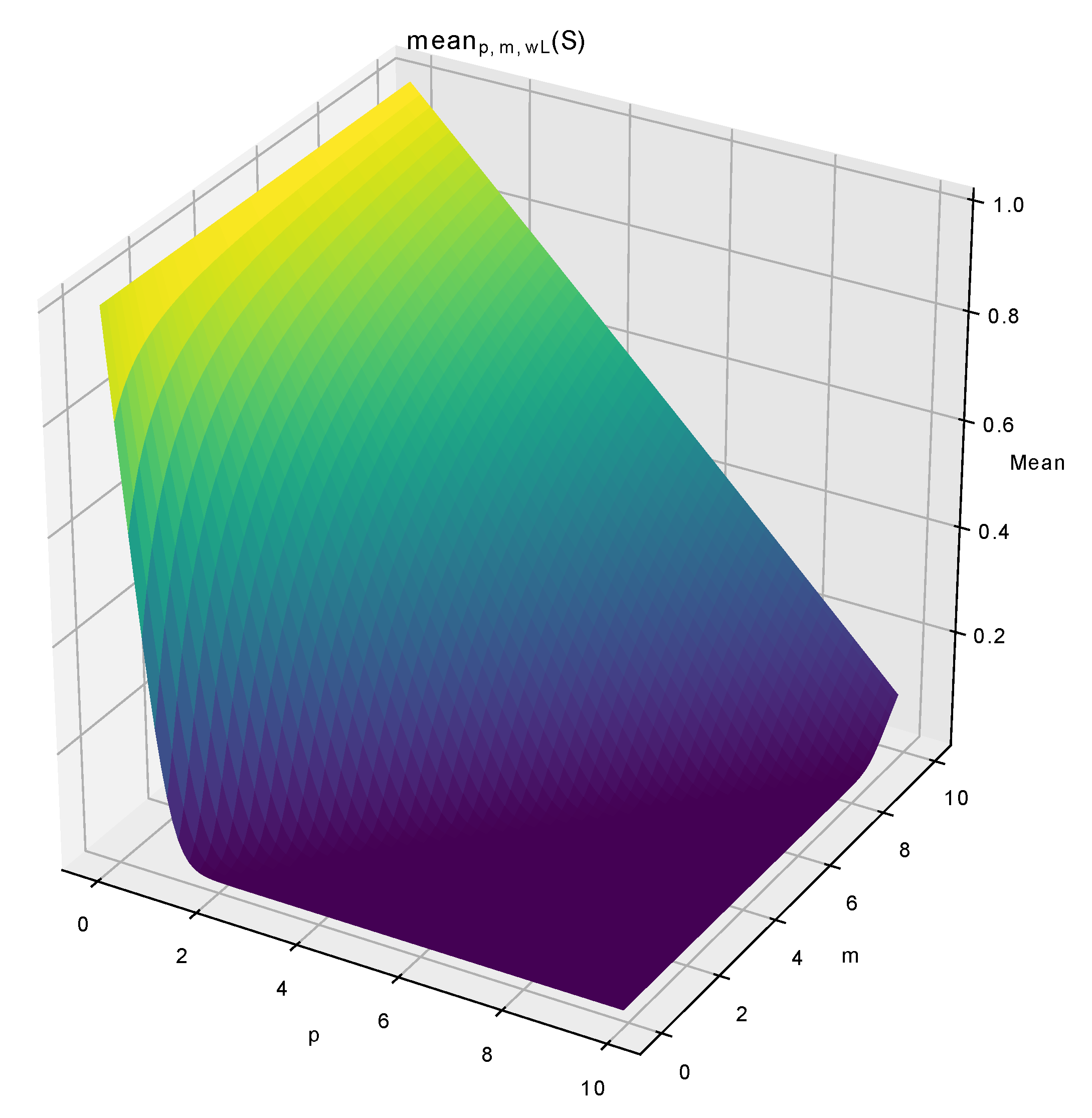
2.3. Proposed Approach: Linear Bias Reduction

One of the problems in parameter adaptation for DE is the existence of structural bias in the parameter adaptation process. For example, the problem of reaching different areas of the search space by DE was discussed in [40]. The JADE and SHADE algorithms used the Lehmer mean [41] instead of the classical arithmetical mean to avoid the structural bias in terms of parameter values, because it is much easier for the algorithm to generate better solutions with smaller F and $Cr$ values than larger F and $Cr$, because smaller parameter values result in more local search, and thus easy improvements. However, such greedy behavior could only be beneficial from a short-term perspective, and only for local search. In [12], the generalized Lehmer mean was proposed, where a larger p parameter in the mean was allowed:

$$mea{n}_{p,m,wL}\left(S\right)=\frac{{\sum }_{j=1}^{\left|S\right|}{w}_j{S}_j^p}{{\sum }_{j=1}^{\left|S\right|}{w}_j{S}_j^m}$$

(17)

The provided equation in its general form defines a group of means, and the values of p and m control the bias towards smaller or larger values. For example, $mea{n}_{0,1,wL}\left(S\right)$ is the harmonic mean, $mea{n}_{0.5,1,wL}\left(S\right)$ the geometric mean, $mea{n}_{1,1,wL}\left(S\right)$ the arithmetic mean, and $mea{n}_{2,1,wL}\left(S\right)$ the contraharmonic mean. Any biased mean could be obtained by setting the parameter values, and the graph of possible $mea{n}_{p,m,wL}$ is presented in Figure 1.

The behavior of the parameter adaptation in DE could be significantly influenced by the newly generated $(M_{F,h},M_{Cr,h})$ values, so that the setting of p and m may influence the sampled F and $Cr$ values, thus leading to a more explorative search, with large p and small m, or a more exploitative search with small p and large m. Further, in this study, the fixed setting of $m=p-1$ will be used, as changing only the p parameter in the Lehmer mean is sufficient to control the biased mean.

Inspired by the idea of linear population size reduction, the Linear Bias Reduction (LBR) technique is proposed. As long as in most cases, the computational resource limit is known, at the beginning of the search process, more exploration is required to find the most promising areas of the search space, while at the end, fast convergence is required. The linear bias reduction starts with a large $p_{max}$ value and gradually decreases the Lehmer mean parameter down to $p_{min}$ as follows:

$$p_g=p_{min}+(p_{max}-p_{min})\ast \frac{NF{E}_{max}-NFE}{NF{E}_{max}}$$

(18)

In this study, the lower limit is set to $p_{min}=1$, which corresponds to the arithmetic mean, while the upper limit $p_{max}$ is changed. The idea of LBR is inherited from the linear parameter reduction scheme L-SHADE algorithm [10] and other studies, such as [25]. The pseudocode of the L-SHADE-LBR is presented in Algorithm 1.

Algorithm 1 L-SHADE-LBR.

1: Set $N{P}_{max}$, $NFE=0$, $NP=N{P}_{max}$D, $NF{E}_{max}$, 2: $H=5$, $A=\varnothing$, $M_{F,r}=0.5$, $M_{Cr,r}=0.8$, $r=1\cdots H$ 3: $M_{F,H+1}=0.9$, $M_{Cr,H+1}=0.9$, $NA=0.7NP$ if jSO 4: $g=0$ 5: Initialize population $P_0=(x_{1,j},\cdots ,x_{NP,j})$ randomly 6: while$NFE<NF{E}_{max}$do 7:     $S_F=\varnothing$, $S_{Cr}=\varnothing$, $\Delta f=\varnothing$ 8:     for $i=1$ to $NP$ do 9:         Current memory index $r=randint[1,H+1]$ 10:         $Cr=randn(M_{Cr,r},0.1)$ 11:         $Cr=min(1,max(0,Cr\left)\right)$ 12:         repeat 13:            $F=randc(M_{F,r},0.1)$ 14:         until $F\ge 0$ 15:         $F=min(1,F)$ 16:         Get $F_w$ if jSO 17:         Limit $Cr$ if jSO 18:         repeat 19:            Randomly generate $r_1$ from $p\%$ best 20:            Randomly generate $r_2$ from $1,N{P}_g$ 21:            Randomly generate $r_3$ from $1,N{A}_g+N{P}_g$ 22:         until $i\ne r_1\ne r_2\ne r_3$ 23:         for j=1 to D do 24:            if jSO then 25:                $v_{i,j}=x_{i,j}+F_w(x_{r_1,j}-x_{i,j})+F(x_{r_2,j}-x_{r_3,j})$ 26:            else 27:                $v_{i,j}=x_{i,j}+F(x_{r_1,j}-x_{i,j})+F(x_{r_2,j}-x_{r_3,j})$ 28:            end if 29:         end for 30:         Get $u_i$ with $Cr$, and calculate $f\left(u_i\right)$ 31:         if $f\left(u_i\right)<f\left(x_i\right)$ then 32:            $x_i\to A$, $x_i=u_i$, $F\to S_F$, $Cr\to S_{Cr}$, $f\left(x_i\right)-f\left(u_i\right)\to \Delta f$ 33:         end if 34:     end for 35:     Update population size $N{P}_{g+1}$ 36:     Recalculate maximum archive size $N{A}_{g+1}$ 37:     Recalculate LBR $p_g$ parameter 38:     if $\left|A\right|>N{A}_{g+1}$ then 39:         Remove random individuals from the archive 40:     end if 41:     if $N{P}_g>N{P}_{g+1}$ then 42:         Remove worst individuals from the population 43:     end if 44:     if $S_F\ne \varnothing$ and $S_{Cr}\ne \varnothing$ then 45:         if DISH then 46:            Update $M_{F,k}$ and $M_{Cr,k}$ with LBR and $\Delta f$ as the weight 47:         else 48:            Update $M_{F,k}$ and $M_{Cr,k}$ with LBR and distance as the weight 49:         end if 50:     end if 51:     $k=k+1$, $g=g+1$ 52:     if $k>H$ then 53:         $k=1$ 54:     end if 55: end while 56: Return best solution $x_{best}$

The next section contains the experimental setup and results of the LBR application to state-of-the-art DE algorithms on the CEC 2017 and 2020 competitions benchmark problems.

3. Results

The evaluation of the linear bias reduction approach was performed on two sets of benchmark problems, in particular the CEC 2017 [5] and CEC 2020 [42] competitions on bound-constrained single-objective optimization. These two sets of test problems were chosen because they represent two different scenarios: the CEC 2017 tests algorithms on 30 different 10, 30, 50, and 100D problems with a limited computational resource, and CEC 2020 has only 10 problems in 5, 10, 15, and 20 dimensions, but allows exponential growth of the computational resource available. For CEC 2017 problems, the resource was set to 10,000D fitness evaluations, and for CEC 2020 it was set to 50,000, ${10}^6$, $3\times {10}^6$, and ${10}^7$ for $5D$, $10D$, $15D$, and $20D$ respectively. All test problems were shifted and rotated to avoid the cheating of the algorithms.

The LBR modification was tested with the L-SHADE, jSO, and DISH algorithms, and the following parameters were set for all algorithms: initial population size $N{P}_{max}=25·log\left(D\right)·\sqrt{D}$ for CEC 2017, $N{P}_{max}=30·D·\sqrt{D}$ for CEC 2020, final population size $N{P}_{min}=4$, $pbest=0.17$, archive size $NA=NP$, number of memory cells $H=5$. The initial value of $p_{m}ax$ in LBR was set to 40 for F update and 32 for $Cr$ update; these values were chosen according to the experimental results reported in [12]. The algorithm was implemented in C++ with GCC and run on a PC with Ubuntu 20.04, an Intel Core i7 8700 k processor, and 32 GB RAM, with the results’ post-processing performed using Python 3.6.

The comparison of the results was performed for L-SHADE, jSO, and DISH with and without LBR. In the case that LBR was not used, the p-values in the Lehmer mean were set to two. The Mann–Whitney statistical test with normal approximation, tie-breaking, and the significance level set to 0.01 was applied to identify the difference between algorithm modifications.

Table 1. Statistical comparison of algorithms with and without LBR, Mann–Whitney test, CEC 2017 problems.

$\mathit{Algorithm}$	$10\mathit{D}$	$30\mathit{D}$	$50\mathit{D}$	$100\mathit{D}$
L-SHADE vs. L-SHADE-LBR	0+/27 = /3−	8+/21 = /1−	17+/12 = /1−	16+/10 = /4−
jSO vs. jSO-LBR	0+/29 = /1−	5+/24 = /1−	10+/20 = /0−	12+/16 = /2−
DISH vs. DISH-LBR	0+/30 = /0−	2+/28 = /0−	4+/25 = /1−	9+/16 = /5−

presents the results of comparing the basic L-SHADE with L-SHADE-LBR on all dimensions of the CEC 2017 test problems. The values in the table show the number of wins (+), non-significant differences (=), and losses (−) summed over all functions.

The results presented in Table 1 show that the LBR gives up to 16 improvements for L-SHADE on 100-dimensional functions and 17 improvements for 50-dimensional functions. The jSO and DISH algorithms, which perform better than L-SHADE, and LBR give smaller improvements for these algorithms. Furthermore, the greater the dimension of the test problems, the more improvements are achieved, i.e., for example, for 10-dimensional problems, the LBR does not deliver any improvements, and for L-SHADE and jSO, there are even several performance deteriorations. Most of the improvements are for multimodal, hybrid, and composition functions.

Table 2. Results for CEC 2017 problems, $10D$.

Function	L-SHADE	jSO	DISH
f1	0.0 ± 0.0	0.0 ± 0.0	0.0 ± 0.0
f2	0.0 ± 0.0	0.0 ± 0.0	0.0 ± 0.0
f3	0.0 ± 0.0	0.0 ± 0.0	0.0 ± 0.0
f4	0.0 ± 0.0	0.0 ± 0.0	0.0 ± 0.0
f5	1.466332$\times {10}^0$ ± 7.966326$\times {10}^{-1}$	1.820984$\times {10}^0$ ± 8.296894$\times {10}^{-1}$	2.028990$\times {10}^0$ ± 9.021237$\times {10}^{-1}$
f6	0.0 ± 0.0	0.0 ± 0.0	0.0 ± 0.0
f7	1.165531$\times {10}^1$ ± 4.999618$\times {10}^{-1}$	1.206354$\times {10}^1$ ± 5.092644$\times {10}^{-1}$	1.202930$\times {10}^1$ ± 5.555746$\times {10}^{-1}$
f8	1.338034$\times {10}^0$ ± 8.316749$\times {10}^{-1}$	1.878932$\times {10}^0$ ± 8.513805$\times {10}^{-1}$	1.853360$\times {10}^0$ ± 1.042962$\times {10}^0$
f9	0.0 ± 0.0	0.0 ± 0.0	0.0 ± 0.0
f10	2.224059$\times {10}^1$ ± 4.032137$\times {10}^1$	1.822742$\times {10}^1$ ± 3.227775$\times {10}^1$	3.377682$\times {10}^1$ ± 5.852428$\times {10}^1$
f11	1.181580$\times {10}^{-1}$ ± 4.216185$\times {10}^{-1}$	1.516416$\times {10}^{-1}$ ± 3.630057$\times {10}^{-1}$	0.0 ± 0.0
f12	1.526398$\times {10}^1$ ± 3.919816$\times {10}^1$	2.734428$\times {10}^{-1}$ ± 1.723809$\times {10}^{-1}$	1.673563$\times {10}^1$ ± 4.110506$\times {10}^1$
f13	2.441962$\times {10}^0$ ± 2.352857$\times {10}^0$	2.474151$\times {10}^0$ ± 2.390764$\times {10}^0$	3.043588$\times {10}^0$ ± 2.362332$\times {10}^0$
f14	4.638013$\times {10}^{-2}$ ± 1.575738$\times {10}^{-1}$	4.747525$\times {10}^{-2}$ ± 1.948063$\times {10}^{-1}$	3.902250$\times {10}^{-2}$ ± 1.931283$\times {10}^{-1}$
f15	1.346569$\times {10}^{-1}$ ± 1.999631$\times {10}^{-1}$	1.225807$\times {10}^{-1}$ ± 1.933628$\times {10}^{-1}$	3.401098$\times {10}^{-1}$ ± 2.058195$\times {10}^{-1}$
f16	4.510030$\times {10}^{-1}$ ± 1.916985$\times {10}^{-1}$	3.580149$\times {10}^{-1}$ ± 1.948515$\times {10}^{-1}$	5.429780$\times {10}^{-1}$ ± 3.146415$\times {10}^{-1}$
f17	1.572282$\times {10}^{-1}$ ± 1.571081$\times {10}^{-1}$	1.409888$\times {10}^{-1}$ ± 1.729228$\times {10}^{-1}$	9.310686$\times {10}^{-1}$ ± 2.782305$\times {10}^0$
f18	2.218042$\times {10}^{-1}$ ± 1.984943$\times {10}^{-1}$	1.422543$\times {10}^{-1}$ ± 1.699201$\times {10}^{-1}$	1.992204$\times {10}^{-1}$ ± 1.953476$\times {10}^{-1}$
f19	9.994697$\times {10}^{-3}$ ± 1.044910$\times {10}^{-2}$	1.164565$\times {10}^{-2}$ ± 1.284938$\times {10}^{-2}$	1.266488$\times {10}^{-2}$ ± 1.275577$\times {10}^{-2}$
f20	6.121039$\times {10}^{-3}$ ± 4.328228$\times {10}^{-2}$	6.121039$\times {10}^{-3}$ ± 4.328228$\times {10}^{-2}$	3.672626$\times {10}^{-1}$ ± 1.476685$\times {10}^{-1}$
f21	1.450680$\times {10}^2$ ± 5.038353$\times {10}^1$	1.506000$\times {10}^2$ ± 5.160565$\times {10}^1$	1.302909$\times {10}^2$ ± 4.692892$\times {10}^1$
f22	1.000056$\times {10}^2$ ± 3.965344$\times {10}^{-2}$	1.000078$\times {10}^2$ ± 5.532071$\times {10}^{-2}$	1.000000$\times {10}^2$ ± 0.0
f23	3.010949$\times {10}^2$ ± 1.487577$\times {10}^0$	3.024831$\times {10}^2$ ± 1.330968$\times {10}^0$	3.010731$\times {10}^2$ ± 1.481965$\times {10}^0$
f24	2.592233$\times {10}^2$ ± 1.036631$\times {10}^2$	2.666515$\times {10}^2$ ± 1.025191$\times {10}^2$	2.748786$\times {10}^2$ ± 9.709894$\times {10}^1$
f25	4.237633$\times {10}^2$ ± 2.248348$\times {10}^1$	4.095063$\times {10}^2$ ± 1.979616$\times {10}^1$	4.095055$\times {10}^2$ ± 1.979735$\times {10}^1$
f26	3.000000$\times {10}^2$ ± 0.0	2.941176$\times {10}^2$ ± 4.159452$\times {10}^1$	3.000000$\times {10}^2$ ± 0.0
f27	3.893875$\times {10}^2$ ± 2.231327$\times {10}^{-1}$	3.892298$\times {10}^2$ ± 5.642233$\times {10}^{-1}$	3.894176$\times {10}^2$ ± 2.032786$\times {10}^{-1}$
f28	4.231326$\times {10}^2$ ± 1.442053$\times {10}^2$	3.578377$\times {10}^2$ ± 1.172708$\times {10}^2$	3.294695$\times {10}^2$ ± 8.948919$\times {10}^1$
f29	2.332684$\times {10}^2$ ± 2.297889$\times {10}^0$	2.334880$\times {10}^2$ ± 1.961177$\times {10}^0$	2.347158$\times {10}^2$ ± 3.342209$\times {10}^0$
f30	3.244280$\times {10}^4$ ± 1.586213$\times {10}^5$	3.945063$\times {10}^2$ ± 2.293938$\times {10}^{-2}$	1.641868$\times {10}^4$ ± 1.133010$\times {10}^5$
Function	L-SHADE-LBR	jSO-LBR	DISH-LBR
f1	0.0 ± 0.0	0.0 ± 0.0	0.0 ± 0.0
f2	0.0 ± 0.0	0.0 ± 0.0	0.0 ± 0.0
f3	0.0 ± 0.0	0.0 ± 0.0	0.0 ± 0.0
f4	0.0 ± 0.0	0.0 ± 0.0	0.0 ± 0.0
f5	1.931394$\times {10}^0$ ± 8.221626$\times {10}^{-1}$	1.833883$\times {10}^0$ ± 8.894004$\times {10}^{-1}$	1.775343$\times {10}^0$ ± 6.914080$\times {10}^{-1}$
f6	0.0 ± 0.0	0.0 ± 0.0	0.0 ± 0.0
f7	1.208296$\times {10}^1$ ± 5.567794$\times {10}^{-1}$	1.216231$\times {10}^1$ ± 5.829416$\times {10}^{-1}$	1.201511$\times {10}^1$ ± 6.008566$\times {10}^{-1}$
f8	2.185022$\times {10}^0$ ± 8.815939$\times {10}^{-1}$	1.853397$\times {10}^0$ ± 9.033848$\times {10}^{-1}$	2.263072$\times {10}^0$ ± 9.046168$\times {10}^{-1}$
f9	0.0 ± 0.0	0.0 ± 0.0	0.0 ± 0.0
f10	3.481015$\times {10}^1$ ± 5.336775$\times {10}^1$	5.487013$\times {10}^1$ ± 8.016722$\times {10}^1$	2.936753$\times {10}^1$ ± 5.244595$\times {10}^1$
f11	0.0 ± 0.0	0.0 ± 0.0	0.0 ± 0.0
f12	7.398462$\times {10}^0$ ± 2.818943$\times {10}^1$	1.674478$\times {10}^1$ ± 4.117527$\times {10}^1$	2.640647$\times {10}^0$ ± 1.640653$\times {10}^1$
f13	2.803025$\times {10}^0$ ± 2.437121$\times {10}^0$	2.675462$\times {10}^0$ ± 2.342831$\times {10}^0$	3.290499$\times {10}^0$ ± 2.290796$\times {10}^0$
f14	1.560720$\times {10}^{-1}$ ± 3.618380$\times {10}^{-1}$	1.462447$\times {10}^{-1}$ ± 3.453513$\times {10}^{-1}$	1.170540$\times {10}^{-1}$ ± 3.205656$\times {10}^{-1}$
f15	2.393091$\times {10}^{-1}$ ± 2.081327$\times {10}^{-1}$	2.935211$\times {10}^{-1}$ ± 2.028156$\times {10}^{-1}$	2.354370$\times {10}^{-1}$ ± 2.096280$\times {10}^{-1}$
f16	7.189243$\times {10}^{-1}$ ± 3.081263$\times {10}^{-1}$	5.107098$\times {10}^{-1}$ ± 2.956673$\times {10}^{-1}$	5.481845$\times {10}^{-1}$ ± 2.890193$\times {10}^{-1}$
f17	4.551964$\times {10}^{-1}$ ± 3.136878$\times {10}^{-1}$	5.855833$\times {10}^{-1}$ ± 3.998470$\times {10}^{-1}$	5.405732$\times {10}^{-1}$ ± 3.427532$\times {10}^{-1}$
f18	2.217356$\times {10}^{-1}$ ± 2.083894$\times {10}^{-1}$	5.850836$\times {10}^{-1}$ ± 2.756645$\times {10}^0$	2.256478$\times {10}^{-1}$ ± 2.133737$\times {10}^{-1}$
f19	1.122558$\times {10}^{-2}$ ± 2.105432$\times {10}^{-2}$	1.145965$\times {10}^{-2}$ ± 1.292694$\times {10}^{-2}$	8.007165$\times {10}^{-3}$ ± 1.032611$\times {10}^{-2}$
f20	8.095347$\times {10}^{-1}$ ± 2.808347$\times {10}^0$	3.672626$\times {10}^{-1}$ ± 1.716079$\times {10}^{-1}$	3.978678$\times {10}^{-1}$ ± 1.524131$\times {10}^{-1}$
f21	1.323348$\times {10}^2$ ± 4.782543$\times {10}^1$	1.363186$\times {10}^2$ ± 4.917879$\times {10}^1$	1.444566$\times {10}^2$ ± 5.104734$\times {10}^1$
f22	1.000079$\times {10}^2$ ± 5.559800$\times {10}^{-2}$	1.000068$\times {10}^2$ ± 4.797234$\times {10}^{-2}$	1.000268$\times {10}^2$ ± 9.379501$\times {10}^{-2}$
f23	3.010237$\times {10}^2$ ± 1.490490$\times {10}^0$	2.955855$\times {10}^2$ ± 4.183554$\times {10}^1$	3.013980$\times {10}^2$ ± 1.570153$\times {10}^0$
f24	3.018687$\times {10}^2$ ± 7.386128$\times {10}^1$	2.656853$\times {10}^2$ ± 1.019472$\times {10}^2$	2.654399$\times {10}^2$ ± 1.018634$\times {10}^2$
f25	4.015055$\times {10}^2$ ± 1.221117$\times {10}^1$	4.059703$\times {10}^2$ ± 1.730538$\times {10}^1$	4.068576$\times {10}^2$ ± 1.801739$\times {10}^1$
f26	3.000000$\times {10}^2$ ± 0.0	3.000000$\times {10}^2$ ± 0.0	3.000000$\times {10}^2$ ± 0.0
f27	3.894635$\times {10}^2$ ± 1.538980$\times {10}^{-1}$	3.893975$\times {10}^2$ ± 2.171814$\times {10}^{-1}$	3.894477$\times {10}^2$ ± 1.761875$\times {10}^{-1}$
f28	3.294695$\times {10}^2$ ± 8.948919$\times {10}^1$	3.361344$\times {10}^2$ ± 9.902322$\times {10}^1$	3.411471$\times {10}^2$ ± 1.032896$\times {10}^2$
f29	2.350070$\times {10}^2$ ± 2.765177$\times {10}^0$	2.345793$\times {10}^2$ ± 3.214256$\times {10}^0$	2.337357$\times {10}^2$ ± 2.522189$\times {10}^0$
f30	3.244093$\times {10}^4$ ± 1.586216$\times {10}^5$	1.641771$\times {10}^4$ ± 1.133012$\times {10}^5$	3.945173$\times {10}^2$ ± 4.152092$\times {10}^{-2}$

,

Table 3. Results for CEC 2017 problems, $30D$.

Function	L-SHADE	jSO	DISH
f1	0.0 ± 0.0	0.0 ± 0.0	0.0 ± 0.0
f2	0.0 ± 0.0	0.0 ± 0.0	0.0 ± 0.0
f3	0.0 ± 0.0	0.0 ± 0.0	0.0 ± 0.0
f4	5.432730$\times {10}^1$ ± 1.761079$\times {10}^1$	5.856160$\times {10}^1$ ± 0.0	5.856160$\times {10}^1$ ± 0.0
f5	7.093248$\times {10}^0$ ± 1.514062$\times {10}^0$	5.984748$\times {10}^0$ ± 1.259837$\times {10}^0$	8.566069$\times {10}^0$ ± 1.414316$\times {10}^0$
f6	1.610282$\times {10}^{-8}$ ± 4.409940$\times {10}^{-8}$	2.683804$\times {10}^{-9}$ ± 1.897736$\times {10}^{-8}$	1.125136$\times {10}^{-7}$ ± 3.080402$\times {10}^{-7}$
f7	3.643252$\times {10}^1$ ± 1.163031$\times {10}^0$	3.635001$\times {10}^1$ ± 1.050653$\times {10}^0$	3.901514$\times {10}^1$ ± 1.897382$\times {10}^0$
f8	7.636827$\times {10}^0$ ± 1.421298$\times {10}^0$	5.947331$\times {10}^0$ ± 1.286650$\times {10}^0$	8.606066$\times {10}^0$ ± 1.668634$\times {10}^0$
f9	0.0 ± 0.0	0.0 ± 0.0	0.0 ± 0.0
f10	1.541919$\times {10}^3$ ± 2.100733$\times {10}^2$	1.588640$\times {10}^3$ ± 2.124062$\times {10}^2$	1.633723$\times {10}^3$ ± 2.570738$\times {10}^2$
f11	1.480573$\times {10}^1$ ± 2.154669$\times {10}^1$	1.286354$\times {10}^1$ ± 2.135075$\times {10}^1$	6.873639$\times {10}^0$ ± 1.395100$\times {10}^1$
f12	9.665733$\times {10}^2$ ± 3.204188$\times {10}^2$	2.131759$\times {10}^2$ ± 1.341268$\times {10}^2$	2.351108$\times {10}^2$ ± 1.392522$\times {10}^2$
f13	1.507205$\times {10}^1$ ± 7.899218$\times {10}^0$	1.747101$\times {10}^1$ ± 5.664911$\times {10}^0$	1.616138$\times {10}^1$ ± 5.997028$\times {10}^0$
f14	2.133530$\times {10}^1$ ± 9.644383$\times {10}^{-1}$	2.136757$\times {10}^1$ ± 3.272063$\times {10}^0$	2.194751$\times {10}^1$ ± 3.183398$\times {10}^0$
f15	2.465098$\times {10}^0$ ± 1.482018$\times {10}^0$	1.524179$\times {10}^0$ ± 9.985145$\times {10}^{-1}$	1.212446$\times {10}^0$ ± 8.005678$\times {10}^{-1}$
f16	6.228463$\times {10}^1$ ± 7.399308$\times {10}^1$	3.557114$\times {10}^1$ ± 3.589944$\times {10}^1$	4.984834$\times {10}^1$ ± 6.435235$\times {10}^1$
f17	3.486476$\times {10}^1$ ± 5.016896$\times {10}^0$	3.316091$\times {10}^1$ ± 5.201363$\times {10}^0$	3.505441$\times {10}^1$ ± 6.723407$\times {10}^0$
f18	2.146325$\times {10}^1$ ± 3.044085$\times {10}^0$	2.077898$\times {10}^1$ ± 4.073286$\times {10}^{-1}$	2.081425$\times {10}^1$ ± 4.281106$\times {10}^{-1}$
f19	5.078805$\times {10}^0$ ± 1.737644$\times {10}^0$	5.462701$\times {10}^0$ ± 1.914274$\times {10}^0$	5.006098$\times {10}^0$ ± 1.699874$\times {10}^0$
f20	3.322552$\times {10}^1$ ± 5.277263$\times {10}^0$	3.011395$\times {10}^1$ ± 4.949041$\times {10}^0$	2.957005$\times {10}^1$ ± 7.071608$\times {10}^0$
f21	2.068744$\times {10}^2$ ± 1.548801$\times {10}^0$	2.063994$\times {10}^2$ ± 1.477586$\times {10}^0$	2.087112$\times {10}^2$ ± 1.873729$\times {10}^0$
f22	1.000000$\times {10}^2$ ± 0.0	1.000000$\times {10}^2$ ± 0.0	1.000000$\times {10}^2$ ± 0.0
f23	3.485940$\times {10}^2$ ± 2.713869$\times {10}^0$	3.483330$\times {10}^2$ ± 2.099438$\times {10}^0$	3.509930$\times {10}^2$ ± 2.924522$\times {10}^0$
f24	4.237707$\times {10}^2$ ± 1.651448$\times {10}^0$	4.251463$\times {10}^2$ ± 1.305455$\times {10}^0$	4.262602$\times {10}^2$ ± 2.262393$\times {10}^0$
f25	3.867463$\times {10}^2$ ± 2.090470$\times {10}^{-2}$	3.867043$\times {10}^2$ ± 1.523778$\times {10}^{-2}$	3.866993$\times {10}^2$ ± 9.419400$\times {10}^{-3}$
f26	9.245550$\times {10}^2$ ± 4.373209$\times {10}^1$	9.254841$\times {10}^2$ ± 3.466222$\times {10}^1$	9.327218$\times {10}^2$ ± 3.297828$\times {10}^1$
f27	5.016845$\times {10}^2$ ± 5.896865$\times {10}^0$	4.926597$\times {10}^2$ ± 7.915101$\times {10}^0$	4.981355$\times {10}^2$ ± 7.186093$\times {10}^0$
f28	3.114948$\times {10}^2$ ± 3.531211$\times {10}^1$	3.064948$\times {10}^2$ ± 2.600802$\times {10}^1$	3.217193$\times {10}^2$ ± 4.403163$\times {10}^1$
f29	4.353955$\times {10}^2$ ± 1.046230$\times {10}^1$	4.392384$\times {10}^2$ ± 1.303416$\times {10}^1$	4.348371$\times {10}^2$ ± 1.639610$\times {10}^1$
f30	1.994910$\times {10}^3$ ± 5.095366$\times {10}^1$	1.969638$\times {10}^3$ ± 1.586864$\times {10}^1$	1.975658$\times {10}^3$ ± 3.868023$\times {10}^1$
Function	L-SHADE-LBR	jSO-LBR	DISH-LBR
f1	0.0 ± 0.0	0.0 ± 0.0	0.0 ± 0.0
f2	0.0 ± 0.0	0.0 ± 0.0	0.0 ± 0.0
f3	0.0 ± 0.0	0.0 ± 0.0	0.0 ± 0.0
f4	5.856160$\times {10}^1$ ± 0.0	5.867054$\times {10}^1$ ± 7.703027$\times {10}^{-1}$	5.856160$\times {10}^1$ ± 0.0
f5	7.138668$\times {10}^0$ ± 1.934874$\times {10}^0$	8.172221$\times {10}^0$ ± 1.624578$\times {10}^0$	7.300936$\times {10}^0$ ± 1.628259$\times {10}^0$
f6	5.733510$\times {10}^{-8}$ ± 1.749795$\times {10}^{-7}$	2.952184$\times {10}^{-8}$ ± 5.629595$\times {10}^{-8}$	5.360755$\times {10}^{-8}$ ± 1.577789$\times {10}^{-7}$
f7	3.729442$\times {10}^1$ ± 1.342658$\times {10}^0$	3.843567$\times {10}^1$ ± 1.603208$\times {10}^0$	3.783948$\times {10}^1$ ± 1.356820$\times {10}^0$
f8	7.340093$\times {10}^0$ ± 1.966085$\times {10}^0$	8.462537$\times {10}^0$ ± 2.018838$\times {10}^0$	7.322912$\times {10}^0$ ± 2.011191$\times {10}^0$
f9	0.0 ± 0.0	0.0 ± 0.0	0.0 ± 0.0
f10	1.568173$\times {10}^3$ ± 2.895061$\times {10}^2$	1.524144$\times {10}^3$ ± 2.684248$\times {10}^2$	1.568425$\times {10}^3$ ± 2.629532$\times {10}^2$
f11	4.027302$\times {10}^0$ ± 8.265100$\times {10}^0$	4.306909$\times {10}^0$ ± 8.200147$\times {10}^0$	7.472353$\times {10}^0$ ± 1.565693$\times {10}^1$
f12	8.106433$\times {10}^1$ ± 7.149354$\times {10}^1$	9.996226$\times {10}^1$ ± 6.182176$\times {10}^1$	6.730995$\times {10}^1$ ± 6.684616$\times {10}^1$
f13	1.552083$\times {10}^1$ ± 6.133034$\times {10}^0$	1.610696$\times {10}^1$ ± 5.854376$\times {10}^0$	1.684447$\times {10}^1$ ± 4.239543$\times {10}^0$
f14	2.171615$\times {10}^1$ ± 1.195599$\times {10}^0$	2.195247$\times {10}^1$ ± 1.241087$\times {10}^0$	2.203156$\times {10}^1$ ± 1.276744$\times {10}^0$
f15	1.184498$\times {10}^0$ ± 7.500999$\times {10}^{-1}$	1.166798$\times {10}^0$ ± 7.381401$\times {10}^{-1}$	1.213596$\times {10}^0$ ± 9.026724$\times {10}^{-1}$
f16	5.466729$\times {10}^1$ ± 7.181852$\times {10}^1$	3.527649$\times {10}^1$ ± 4.731054$\times {10}^1$	3.623068$\times {10}^1$ ± 5.130314$\times {10}^1$
f17	3.449224$\times {10}^1$ ± 7.695939$\times {10}^0$	3.388604$\times {10}^1$ ± 6.728233$\times {10}^0$	3.355475$\times {10}^1$ ± 7.485698$\times {10}^0$
f18	2.084219$\times {10}^1$ ± 3.720811$\times {10}^{-1}$	2.006454$\times {10}^1$ ± 3.965811$\times {10}^0$	2.045489$\times {10}^1$ ± 2.704982$\times {10}^0$
f19	4.817716$\times {10}^0$ ± 1.898779$\times {10}^0$	4.076852$\times {10}^0$ ± 1.356127$\times {10}^0$	4.425025$\times {10}^0$ ± 1.967937$\times {10}^0$
f20	2.972537$\times {10}^1$ ± 8.035391$\times {10}^0$	2.704956$\times {10}^1$ ± 6.845223$\times {10}^0$	2.679755$\times {10}^1$ ± 7.130091$\times {10}^0$
f21	2.083516$\times {10}^2$ ± 1.807313$\times {10}^0$	2.085552$\times {10}^2$ ± 1.968052$\times {10}^0$	2.080673$\times {10}^2$ ± 2.171051$\times {10}^0$
f22	1.000000$\times {10}^2$ ± 0.0	1.000000$\times {10}^2$ ± 0.0	1.000000$\times {10}^2$ ± 0.0
f23	3.505319$\times {10}^2$ ± 3.690104$\times {10}^0$	3.507215$\times {10}^2$ ± 3.276329$\times {10}^0$	3.498206$\times {10}^2$ ± 3.709504$\times {10}^0$
f24	4.263549$\times {10}^2$ ± 2.213716$\times {10}^0$	4.259219$\times {10}^2$ ± 1.872762$\times {10}^0$	4.262288$\times {10}^2$ ± 2.572837$\times {10}^0$
f25	3.866960$\times {10}^2$ ± 7.127660$\times {10}^{-3}$	3.866957$\times {10}^2$ ± 5.585311$\times {10}^{-3}$	3.866962$\times {10}^2$ ± 6.091826$\times {10}^{-3}$
f26	9.561221$\times {10}^2$ ± 4.264016$\times {10}^1$	9.313090$\times {10}^2$ ± 4.626237$\times {10}^1$	9.371625$\times {10}^2$ ± 4.567299$\times {10}^1$
f27	4.932655$\times {10}^2$ ± 7.774858$\times {10}^0$	4.932667$\times {10}^2$ ± 7.143169$\times {10}^0$	4.899617$\times {10}^2$ ± 6.927315$\times {10}^0$
f28	3.042600$\times {10}^2$ ± 2.111257$\times {10}^1$	3.085200$\times {10}^2$ ± 2.924355$\times {10}^1$	3.000000$\times {10}^2$ ± 0.0
f29	4.348186$\times {10}^2$ ± 1.955936$\times {10}^1$	4.340111$\times {10}^2$ ± 1.408097$\times {10}^1$	4.350100$\times {10}^2$ ± 1.643612$\times {10}^1$
f30	1.969240$\times {10}^3$ ± 9.962199$\times {10}^0$	1.972825$\times {10}^3$ ± 2.132789$\times {10}^1$	1.966696$\times {10}^3$ ± 9.911583$\times {10}^0$

,

Table 4. Results for CEC 2020 problems, $50D$.

Function	L-SHADE	jSO	DISH
f1	0.0 ± 0.0	0.0 ± 0.0	0.0 ± 0.0
f2	0.0 ± 0.0	0.0 ± 0.0	0.0 ± 0.0
f3	0.0 ± 0.0	0.0 ± 0.0	0.0 ± 0.0
f4	5.235449$\times {10}^1$ ± 4.437343$\times {10}^1$	5.987294$\times {10}^1$ ± 4.656380$\times {10}^1$	5.533534$\times {10}^1$ ± 4.638192$\times {10}^1$
f5	1.858622$\times {10}^1$ ± 2.721102$\times {10}^0$	1.090016$\times {10}^1$ ± 2.044454$\times {10}^0$	1.643115$\times {10}^1$ ± 2.349557$\times {10}^0$
f6	1.826999$\times {10}^{-4}$ ± 9.247796$\times {10}^{-4}$	3.321219$\times {10}^{-7}$ ± 7.189487$\times {10}^{-7}$	1.159359$\times {10}^{-6}$ ± 1.645192$\times {10}^{-6}$
f7	6.474578$\times {10}^1$ ± 1.859098$\times {10}^0$	6.125818$\times {10}^1$ ± 1.330959$\times {10}^0$	6.533251$\times {10}^1$ ± 2.386148$\times {10}^0$
f8	1.786065$\times {10}^1$ ± 2.476184$\times {10}^0$	1.059279$\times {10}^1$ ± 1.794339$\times {10}^0$	1.642296$\times {10}^1$ ± 2.506320$\times {10}^0$
f9	0.0 ± 0.0	0.0 ± 0.0	0.0 ± 0.0
f10	3.145981$\times {10}^3$ ± 3.519306$\times {10}^2$	3.289575$\times {10}^3$ ± 3.466515$\times {10}^2$	3.287218$\times {10}^3$ ± 3.405172$\times {10}^2$
f11	4.479648$\times {10}^1$ ± 7.262966$\times {10}^0$	2.847299$\times {10}^1$ ± 3.609160$\times {10}^0$	2.765099$\times {10}^1$ ± 3.060072$\times {10}^0$
f12	2.211379$\times {10}^3$ ± 5.051756$\times {10}^2$	1.791286$\times {10}^3$ ± 4.034954$\times {10}^2$	1.688626$\times {10}^3$ ± 4.222375$\times {10}^2$
f13	5.887959$\times {10}^1$ ± 3.102544$\times {10}^1$	5.325204$\times {10}^1$ ± 2.649015$\times {10}^1$	3.130917$\times {10}^1$ ± 1.675635$\times {10}^1$
f14	2.896163$\times {10}^1$ ± 3.059013$\times {10}^0$	2.516679$\times {10}^1$ ± 1.954335$\times {10}^0$	2.528063$\times {10}^1$ ± 2.405140$\times {10}^0$
f15	3.628762$\times {10}^1$ ± 8.435876$\times {10}^0$	2.536133$\times {10}^1$ ± 3.286879$\times {10}^0$	2.407813$\times {10}^1$ ± 2.946462$\times {10}^0$
f16	3.678356$\times {10}^2$ ± 8.492899$\times {10}^1$	3.514246$\times {10}^2$ ± 1.238785$\times {10}^2$	4.255240$\times {10}^2$ ± 1.338552$\times {10}^2$
f17	3.210085$\times {10}^2$ ± 8.169067$\times {10}^1$	2.288290$\times {10}^2$ ± 7.119400$\times {10}^1$	2.673055$\times {10}^2$ ± 7.762843$\times {10}^1$
f18	3.657321$\times {10}^1$ ± 9.959862$\times {10}^0$	2.552774$\times {10}^1$ ± 2.227834$\times {10}^0$	2.530384$\times {10}^1$ ± 1.768854$\times {10}^0$
f19	2.229348$\times {10}^1$ ± 5.693372$\times {10}^0$	1.598069$\times {10}^1$ ± 3.193897$\times {10}^0$	1.473478$\times {10}^1$ ± 2.609984$\times {10}^0$
f20	1.403643$\times {10}^2$ ± 6.340770$\times {10}^1$	1.545319$\times {10}^2$ ± 5.105286$\times {10}^1$	1.195946$\times {10}^2$ ± 5.365881$\times {10}^1$
f21	2.167895$\times {10}^2$ ± 2.526317$\times {10}^0$	2.112500$\times {10}^2$ ± 2.551442$\times {10}^0$	2.176929$\times {10}^2$ ± 2.782886$\times {10}^0$
f22	1.090866$\times {10}^3$ ± 1.616684$\times {10}^3$	2.492513$\times {10}^3$ ± 1.798316$\times {10}^3$	2.005652$\times {10}^3$ ± 1.887346$\times {10}^3$
f23	4.306553$\times {10}^2$ ± 5.383210$\times {10}^0$	4.292150$\times {10}^2$ ± 5.785777$\times {10}^0$	4.311355$\times {10}^2$ ± 6.917497$\times {10}^0$
f24	5.070785$\times {10}^2$ ± 3.570835$\times {10}^0$	5.065977$\times {10}^2$ ± 3.750386$\times {10}^0$	5.083627$\times {10}^2$ ± 4.562561$\times {10}^0$
f25	5.403542$\times {10}^2$ ± 2.684350$\times {10}^1$	4.823364$\times {10}^2$ ± 6.109998$\times {10}^0$	4.811605$\times {10}^2$ ± 3.115865$\times {10}^0$
f26	1.222280$\times {10}^3$ ± 5.892037$\times {10}^1$	1.137749$\times {10}^3$ ± 5.618732$\times {10}^1$	1.127770$\times {10}^3$ ± 5.926815$\times {10}^1$
f27	5.254951$\times {10}^2$ ± 1.084758$\times {10}^1$	5.098628$\times {10}^2$ ± 9.343850$\times {10}^0$	5.120206$\times {10}^2$ ± 1.296607$\times {10}^1$
f28	4.901310$\times {10}^2$ ± 2.315774$\times {10}^1$	4.625180$\times {10}^2$ ± 1.261646$\times {10}^1$	4.598068$\times {10}^2$ ± 6.772419$\times {10}^0$
f29	3.695921$\times {10}^2$ ± 2.035753$\times {10}^1$	3.693345$\times {10}^2$ ± 1.245696$\times {10}^1$	3.660005$\times {10}^2$ ± 1.532970$\times {10}^1$
f30	6.485235$\times {10}^5$ ± 6.118087$\times {10}^4$	6.093376$\times {10}^5$ ± 3.282382$\times {10}^4$	6.120136$\times {10}^5$ ± 4.048972$\times {10}^4$
Function	L-SHADE-LBR	jSO-LBR	DISH-LBR
f1	0.0 ± 0.0	0.0 ± 0.0	0.0 ± 0.0
f2	0.0 ± 0.0	0.0 ± 0.0	0.0 ± 0.0
f3	0.0 ± 0.0	0.0 ± 0.0	0.0 ± 0.0
f4	6.309933$\times {10}^1$ ± 4.861348$\times {10}^1$	5.566785$\times {10}^1$ ± 4.698233$\times {10}^1$	4.758795$\times {10}^1$ ± 4.251127$\times {10}^1$
f5	1.151320$\times {10}^1$ ± 2.639832$\times {10}^0$	1.326464$\times {10}^1$ ± 2.814235$\times {10}^0$	1.142791$\times {10}^1$ ± 3.021920$\times {10}^0$
f6	8.654442$\times {10}^{-7}$ ± 9.973005$\times {10}^{-7}$	3.268284$\times {10}^{-7}$ ± 6.168995$\times {10}^{-7}$	1.133130$\times {10}^{-6}$ ± 1.432097$\times {10}^{-6}$
f7	6.261671$\times {10}^1$ ± 2.090590$\times {10}^0$	6.495951$\times {10}^1$ ± 2.964682$\times {10}^0$	6.340675$\times {10}^1$ ± 2.379764$\times {10}^0$
f8	1.129984$\times {10}^1$ ± 2.991564$\times {10}^0$	1.405517$\times {10}^1$ ± 2.486846$\times {10}^0$	1.080723$\times {10}^1$ ± 2.867020$\times {10}^0$
f9	0.0 ± 0.0	0.0 ± 0.0	0.0 ± 0.0
f10	3.291896$\times {10}^3$ ± 3.546988$\times {10}^2$	3.251439$\times {10}^3$ ± 3.159284$\times {10}^2$	3.280655$\times {10}^3$ ± 3.345557$\times {10}^2$
f11	2.434579$\times {10}^1$ ± 3.577627$\times {10}^0$	2.366605$\times {10}^1$ ± 3.226247$\times {10}^0$	2.435336$\times {10}^1$ ± 3.915678$\times {10}^0$
f12	1.221989$\times {10}^3$ ± 3.673815$\times {10}^2$	1.231565$\times {10}^3$ ± 3.631003$\times {10}^2$	1.101802$\times {10}^3$ ± 2.769593$\times {10}^2$
f13	2.996118$\times {10}^1$ ± 1.994031$\times {10}^1$	2.509417$\times {10}^1$ ± 2.325881$\times {10}^1$	2.884285$\times {10}^1$ ± 2.311451$\times {10}^1$
f14	2.469884$\times {10}^1$ ± 2.257149$\times {10}^0$	2.434175$\times {10}^1$ ± 2.010046$\times {10}^0$	2.408265$\times {10}^1$ ± 2.364445$\times {10}^0$
f15	2.124024$\times {10}^1$ ± 1.743464$\times {10}^0$	2.098253$\times {10}^1$ ± 1.794117$\times {10}^0$	2.006068$\times {10}^1$ ± 1.504636$\times {10}^0$
f16	3.748420$\times {10}^2$ ± 1.328029$\times {10}^2$	4.129801$\times {10}^2$ ± 1.369084$\times {10}^2$	3.800765$\times {10}^2$ ± 1.210071$\times {10}^2$
f17	2.439444$\times {10}^2$ ± 8.263835$\times {10}^1$	2.795374$\times {10}^2$ ± 1.127910$\times {10}^2$	2.368689$\times {10}^2$ ± 9.354595$\times {10}^1$
f18	2.261803$\times {10}^1$ ± 1.476114$\times {10}^0$	2.290233$\times {10}^1$ ± 1.433200$\times {10}^0$	2.229708$\times {10}^1$ ± 9.553674$\times {10}^{-1}$
f19	1.152990$\times {10}^1$ ± 2.462608$\times {10}^0$	1.167486$\times {10}^1$ ± 3.407432$\times {10}^0$	1.085855$\times {10}^1$ ± 2.264789$\times {10}^0$
f20	1.311696$\times {10}^2$ ± 5.913158$\times {10}^1$	1.463096$\times {10}^2$ ± 8.239168$\times {10}^1$	1.140987$\times {10}^2$ ± 5.954660$\times {10}^1$
f21	2.134822$\times {10}^2$ ± 3.087330$\times {10}^0$	2.150670$\times {10}^2$ ± 2.682522$\times {10}^0$	2.122163$\times {10}^2$ ± 3.509845$\times {10}^0$
f22	2.137994$\times {10}^3$ ± 1.867652$\times {10}^3$	1.807509$\times {10}^3$ ± 1.762836$\times {10}^3$	1.971311$\times {10}^3$ ± 1.854554$\times {10}^3$
f23	4.291962$\times {10}^2$ ± 6.293038$\times {10}^0$	4.299165$\times {10}^2$ ± 5.907164$\times {10}^0$	4.310311$\times {10}^2$ ± 8.161084$\times {10}^0$
f24	5.082245$\times {10}^2$ ± 4.368923$\times {10}^0$	5.068221$\times {10}^2$ ± 3.243129$\times {10}^0$	5.076325$\times {10}^2$ ± 4.327285$\times {10}^0$
f25	4.806366$\times {10}^2$ ± 2.299212$\times {10}^0$	4.809218$\times {10}^2$ ± 2.728328$\times {10}^0$	4.804641$\times {10}^2$ ± 1.608251$\times {10}^0$
f26	1.137797$\times {10}^3$ ± 6.906183$\times {10}^1$	1.140350$\times {10}^3$ ± 5.343276$\times {10}^1$	1.129101$\times {10}^3$ ± 6.948572$\times {10}^1$
f27	5.091280$\times {10}^2$ ± 1.372703$\times {10}^1$	5.062935$\times {10}^2$ ± 8.969971$\times {10}^0$	5.027209$\times {10}^2$ ± 1.332971$\times {10}^1$
f28	4.588490$\times {10}^2$ ± 5.684342$\times {10}^{-14}$	4.588490$\times {10}^2$ ± 5.684342$\times {10}^{-14}$	4.588490$\times {10}^2$ ± 5.684342$\times {10}^{-14}$
f29	3.689658$\times {10}^2$ ± 1.435579$\times {10}^1$	3.645692$\times {10}^2$ ± 1.356443$\times {10}^1$	3.618460$\times {10}^2$ ± 1.293478$\times {10}^1$
f30	6.042557$\times {10}^5$ ± 3.470244$\times {10}^4$	6.052686$\times {10}^5$ ± 2.884529$\times {10}^4$	6.030053$\times {10}^5$ ± 3.227074$\times {10}^4$

and

Table 5. Results for CEC 2017 problems, $100D$.

Function	L-SHADE	jSO	DISH
f1	0.0 ± 0.0	0.0 ± 0.0	0.0 ± 0.0
f2	2.115272$\times {10}^1$ ± 7.398144$\times {10}^1$	3.621475$\times {10}^5$ ± 2.321462$\times {10}^6$	2.681979$\times {10}^1$ ± 1.323709$\times {10}^2$
f3	2.318827$\times {10}^{-6}$ ± 3.171098$\times {10}^{-6}$	1.189379$\times {10}^{-5}$ ± 1.466348$\times {10}^{-5}$	1.798921$\times {10}^{-7}$ ± 2.335796$\times {10}^{-7}$
f4	1.058027$\times {10}^2$ ± 6.168533$\times {10}^1$	1.841503$\times {10}^2$ ± 3.456924$\times {10}^1$	1.985144$\times {10}^2$ ± 1.507302$\times {10}^1$
f5	6.018822$\times {10}^1$ ± 7.650742$\times {10}^0$	2.881188$\times {10}^1$ ± 5.095198$\times {10}^0$	3.903405$\times {10}^1$ ± 4.302748$\times {10}^0$
f6	2.768146$\times {10}^{-2}$ ± 2.094528$\times {10}^{-2}$	6.501323$\times {10}^{-4}$ ± 1.049251$\times {10}^{-3}$	1.157600$\times {10}^{-4}$ ± 3.452856$\times {10}^{-4}$
f7	1.548649$\times {10}^2$ ± 6.128553$\times {10}^0$	1.344337$\times {10}^2$ ± 3.132118$\times {10}^0$	1.395379$\times {10}^2$ ± 5.342167$\times {10}^0$
f8	5.553710$\times {10}^1$ ± 7.466852$\times {10}^0$	2.763175$\times {10}^1$ ± 4.045294$\times {10}^0$	3.991552$\times {10}^1$ ± 3.695467$\times {10}^0$
f9	0.0 ± 0.0	0.0 ± 0.0	0.0 ± 0.0
f10	9.323340$\times {10}^3$ ± 4.989688$\times {10}^2$	9.672592$\times {10}^3$ ± 5.809016$\times {10}^2$	9.829538$\times {10}^3$ ± 4.826719$\times {10}^2$
f11	4.977651$\times {10}^2$ ± 1.154684$\times {10}^2$	1.398680$\times {10}^2$ ± 4.061085$\times {10}^1$	1.037060$\times {10}^2$ ± 2.911234$\times {10}^1$
f12	2.859917$\times {10}^4$ ± 1.360122$\times {10}^4$	1.881319$\times {10}^4$ ± 9.745573$\times {10}^3$	1.760383$\times {10}^4$ ± 7.710254$\times {10}^3$
f13	4.605786$\times {10}^2$ ± 2.511310$\times {10}^2$	1.473008$\times {10}^2$ ± 3.623802$\times {10}^1$	1.498773$\times {10}^2$ ± 3.307054$\times {10}^1$
f14	2.557099$\times {10}^2$ ± 4.291528$\times {10}^1$	7.044519$\times {10}^1$ ± 1.206246$\times {10}^1$	6.030425$\times {10}^1$ ± 9.448970$\times {10}^0$
f15	2.477823$\times {10}^2$ ± 5.117302$\times {10}^1$	2.053792$\times {10}^2$ ± 4.548641$\times {10}^1$	1.577945$\times {10}^2$ ± 3.308829$\times {10}^1$
f16	1.556113$\times {10}^3$ ± 2.800367$\times {10}^2$	1.608918$\times {10}^3$ ± 2.842634$\times {10}^2$	1.718316$\times {10}^3$ ± 3.021229$\times {10}^2$
f17	1.202785$\times {10}^3$ ± 1.818120$\times {10}^2$	1.096731$\times {10}^3$ ± 2.224261$\times {10}^2$	1.205546$\times {10}^3$ ± 1.764183$\times {10}^2$
f18	2.505036$\times {10}^2$ ± 5.809274$\times {10}^1$	2.154752$\times {10}^2$ ± 5.280900$\times {10}^1$	1.852876$\times {10}^2$ ± 4.461551$\times {10}^1$
f19	1.872595$\times {10}^2$ ± 2.511073$\times {10}^1$	1.325648$\times {10}^2$ ± 2.787079$\times {10}^1$	9.679019$\times {10}^1$ ± 2.009190$\times {10}^1$
f20	1.315492$\times {10}^3$ ± 2.221504$\times {10}^2$	1.415311$\times {10}^3$ ± 1.801826$\times {10}^2$	1.400301$\times {10}^3$ ± 1.908523$\times {10}^2$
f21	2.683218$\times {10}^2$ ± 5.769608$\times {10}^0$	2.521659$\times {10}^2$ ± 4.632993$\times {10}^0$	2.616113$\times {10}^2$ ± 6.682406$\times {10}^0$
f22	1.040296$\times {10}^4$ ± 5.472091$\times {10}^2$	1.082725$\times {10}^4$ ± 3.703361$\times {10}^2$	1.069680$\times {10}^4$ ± 5.856186$\times {10}^2$
f23	5.802729$\times {10}^2$ ± 1.030188$\times {10}^1$	5.690771$\times {10}^2$ ± 1.305997$\times {10}^1$	5.676531$\times {10}^2$ ± 1.120739$\times {10}^1$
f24	9.211472$\times {10}^2$ ± 1.071240$\times {10}^1$	9.011854$\times {10}^2$ ± 8.832015$\times {10}^0$	9.021128$\times {10}^2$ ± 8.999005$\times {10}^0$
f25	7.374379$\times {10}^2$ ± 3.838504$\times {10}^1$	7.328269$\times {10}^2$ ± 3.355738$\times {10}^1$	7.234544$\times {10}^2$ ± 4.379540$\times {10}^1$
f26	3.491742$\times {10}^3$ ± 1.258458$\times {10}^2$	3.205070$\times {10}^3$ ± 9.033496$\times {10}^1$	3.225848$\times {10}^3$ ± 9.340949$\times {10}^1$
f27	6.178230$\times {10}^2$ ± 2.298992$\times {10}^1$	5.971925$\times {10}^2$ ± 2.012176$\times {10}^1$	5.780971$\times {10}^2$ ± 1.877897$\times {10}^1$
f28	5.361838$\times {10}^2$ ± 3.127036$\times {10}^1$	5.351704$\times {10}^2$ ± 2.750945$\times {10}^1$	5.269297$\times {10}^2$ ± 2.456277$\times {10}^1$
f29	1.243196$\times {10}^3$ ± 1.472281$\times {10}^2$	1.155445$\times {10}^3$ ± 1.799635$\times {10}^2$	1.289836$\times {10}^3$ ± 2.137914$\times {10}^2$
f30	2.440230$\times {10}^3$ ± 1.492281$\times {10}^2$	2.361227$\times {10}^3$ ± 1.419884$\times {10}^2$	2.356999$\times {10}^3$ ± 1.423812$\times {10}^2$
Function	L-SHADE-LBR	jSO-LBR	DISH-LBR
f1	0.0 ± 0.0	0.0 ± 0.0	5.038721$\times {10}^{-7}$ ± 1.209810$\times {10}^{-6}$
f2	1.673566$\times {10}^4$ ± 8.143557$\times {10}^4$	2.786236$\times {10}^3$ ± 1.828659$\times {10}^4$	1.619229$\times {10}^5$ ± 9.865543$\times {10}^5$
f3	2.598700$\times {10}^{-6}$ ± 3.046766$\times {10}^{-6}$	5.200551$\times {10}^{-6}$ ± 5.106623$\times {10}^{-6}$	1.867233$\times {10}^{-4}$ ± 2.098053$\times {10}^{-4}$
f4	2.001814$\times {10}^2$ ± 1.061642$\times {10}^1$	2.026510$\times {10}^2$ ± 1.067640$\times {10}^1$	1.986945$\times {10}^2$ ± 9.981837$\times {10}^0$
f5	2.282564$\times {10}^1$ ± 5.374418$\times {10}^0$	2.973385$\times {10}^1$ ± 5.185268$\times {10}^0$	2.126504$\times {10}^1$ ± 4.943471$\times {10}^0$
f6	4.324963$\times {10}^{-5}$ ± 3.097421$\times {10}^{-5}$	1.037825$\times {10}^{-5}$ ± 1.022042$\times {10}^{-5}$	2.023262$\times {10}^{-5}$ ± 1.675807$\times {10}^{-5}$
f7	1.258454$\times {10}^2$ ± 4.037642$\times {10}^0$	1.316895$\times {10}^2$ ± 4.837579$\times {10}^0$	1.250752$\times {10}^2$ ± 5.169489$\times {10}^0$
f8	2.262054$\times {10}^1$ ± 5.062372$\times {10}^0$	2.849150$\times {10}^1$ ± 5.048100$\times {10}^0$	2.191965$\times {10}^1$ ± 4.776998$\times {10}^0$
f9	0.0 ± 0.0	0.0 ± 0.0	0.0 ± 0.0
f10	1.003350$\times {10}^4$ ± 5.181942$\times {10}^2$	9.919141$\times {10}^3$ ± 5.053399$\times {10}^2$	9.883996$\times {10}^3$ ± 5.542053$\times {10}^2$
f11	5.681264$\times {10}^1$ ± 2.615972$\times {10}^1$	6.601018$\times {10}^1$ ± 3.161370$\times {10}^1$	6.454649$\times {10}^1$ ± 3.386242$\times {10}^1$
f12	1.084098$\times {10}^4$ ± 4.835960$\times {10}^3$	1.171083$\times {10}^4$ ± 5.317012$\times {10}^3$	1.629061$\times {10}^4$ ± 7.410286$\times {10}^3$
f13	1.252693$\times {10}^2$ ± 2.955466$\times {10}^1$	1.221712$\times {10}^2$ ± 3.504948$\times {10}^1$	1.239350$\times {10}^2$ ± 3.319592$\times {10}^1$
f14	4.026492$\times {10}^1$ ± 4.654467$\times {10}^0$	3.953127$\times {10}^1$ ± 4.084129$\times {10}^0$	3.520826$\times {10}^1$ ± 3.548234$\times {10}^0$
f15	9.450216$\times {10}^1$ ± 3.081027$\times {10}^1$	9.918180$\times {10}^1$ ± 3.475378$\times {10}^1$	9.316875$\times {10}^1$ ± 3.463347$\times {10}^1$
f16	1.762196$\times {10}^3$ ± 2.895494$\times {10}^2$	1.653987$\times {10}^3$ ± 3.149891$\times {10}^2$	1.610269$\times {10}^3$ ± 3.171456$\times {10}^2$
f17	1.177577$\times {10}^3$ ± 2.796055$\times {10}^2$	1.214972$\times {10}^3$ ± 2.455955$\times {10}^2$	1.195693$\times {10}^3$ ± 2.879482$\times {10}^2$
f18	9.865988$\times {10}^1$ ± 2.318114$\times {10}^1$	9.849790$\times {10}^1$ ± 2.673075$\times {10}^1$	8.753706$\times {10}^1$ ± 1.577905$\times {10}^1$
f19	5.375456$\times {10}^1$ ± 6.426384$\times {10}^0$	5.332317$\times {10}^1$ ± 6.965122$\times {10}^0$	4.849865$\times {10}^1$ ± 6.528906$\times {10}^0$
f20	1.361891$\times {10}^3$ ± 2.361198$\times {10}^2$	1.382355$\times {10}^3$ ± 1.833415$\times {10}^2$	1.440578$\times {10}^3$ ± 2.375126$\times {10}^2$
f21	2.498712$\times {10}^2$ ± 4.793399$\times {10}^0$	2.528137$\times {10}^2$ ± 6.324763$\times {10}^0$	2.474338$\times {10}^2$ ± 4.624437$\times {10}^0$
f22	1.089671$\times {10}^4$ ± 5.882543$\times {10}^2$	1.056397$\times {10}^4$ ± 5.692429$\times {10}^2$	1.064701$\times {10}^4$ ± 6.777621$\times {10}^2$
f23	5.685648$\times {10}^2$ ± 1.051014$\times {10}^1$	5.673360$\times {10}^2$ ± 9.183117$\times {10}^0$	5.682635$\times {10}^2$ ± 9.777963$\times {10}^0$
f24	8.976863$\times {10}^2$ ± 8.162956$\times {10}^0$	8.979166$\times {10}^2$ ± 6.615433$\times {10}^0$	8.970015$\times {10}^2$ ± 7.936307$\times {10}^0$
f25	6.981912$\times {10}^2$ ± 4.440744$\times {10}^1$	7.117357$\times {10}^2$ ± 4.069772$\times {10}^1$	6.780342$\times {10}^2$ ± 4.988064$\times {10}^1$
f26	3.120648$\times {10}^3$ ± 8.549825$\times {10}^1$	3.144199$\times {10}^3$ ± 9.002875$\times {10}^1$	3.076108$\times {10}^3$ ± 9.972924$\times {10}^1$
f27	5.746185$\times {10}^2$ ± 2.402400$\times {10}^1$	5.729895$\times {10}^2$ ± 1.855867$\times {10}^1$	5.600763$\times {10}^2$ ± 2.094522$\times {10}^1$
f28	5.161411$\times {10}^2$ ± 1.977592$\times {10}^1$	5.203338$\times {10}^2$ ± 2.475601$\times {10}^1$	5.205190$\times {10}^2$ ± 2.297309$\times {10}^1$
f29	1.268410$\times {10}^3$ ± 2.138615$\times {10}^2$	1.240134$\times {10}^3$ ± 1.761199$\times {10}^2$	1.265436$\times {10}^3$ ± 1.745885$\times {10}^2$
f30	2.301197$\times {10}^3$ ± 1.302743$\times {10}^2$	2.257047$\times {10}^3$ ± 1.092659$\times {10}^2$	2.254460$\times {10}^3$ ± 1.133409$\times {10}^2$

contain the results for all CEC 2017 functions for all dimensions. The results presented in Table 2, Table 3, Table 4 and Table 5 show that the linear bias reduction has the largest influence on 50- and 100-dimensional functions. Best values for each function are highlighted with bold.

Table 6. Statistical comparison of algorithms with and without LBR, Mann–Whitney test, CEC 2020 problems.

$\mathit{Algorithm}$	$5\mathit{D}$	$10\mathit{D}$	$15\mathit{D}$	$20\mathit{D}$
L-SHADE vs. L-SHADE-LBR	0+/8 = /1-	2+/7 = /1-	2+/6 = /2-	1+/8 = /1-
jSO vs. jSO-LBR	0+/9 = /0-	1+/9 = /0-	3+/7 = /0-	2+/8 = /0-
DISH vs. DISH-LBR	0+/9 = /0-	2+/8 = /0-	2+/7 = /1-	2+/8 = /0-

contains the Mann–Whitney tests for the CEC 2020 benchmark problems.

The results presented in Table 6 shows that the LBR allows up to two improvements for the L-SHADE algorithm for $10D$, $15D$, and $20D$, and one decreased performance. The improvements were mainly for functions f5 and f6, i.e., hybrid functions. For the jSO algorithm, there were up to three improvements for 15D, and for the DISH algorithm, which also included jSO adaptations, there were up to two improvements, which were observed for f5, f6, and f7.

Table 7. Results for CEC 2020 problems, $5D$.

Func.	L-SHADE	jSO	DISH
f1	0.0 ± 0.0	0.0 ± 0.0	0.0 ± 0.0
f2	2.10142$\times {10}^{-1}$ ± 9.06803$\times {10}^{-2}$	4.26469$\times {10}^{-1}$ ± 4.06753$\times {10}^{-1}$	3.67067$\times {10}^{-1}$ ± 2.07562$\times {10}^{-1}$
f3	5.28447$\times {10}^0$ ± 1.11465$\times {10}^{-1}$	5.25455$\times {10}^0$ ± 1.00384$\times {10}^0$	5.26472$\times {10}^0$ ± 2.30645$\times {10}^{-1}$
f4	1.12273$\times {10}^{-1}$ ± 2.46869$\times {10}^{-2}$	9.77072$\times {10}^{-2}$ ± 4.59113$\times {10}^{-2}$	1.09207$\times {10}^{-1}$ ± 4.67916$\times {10}^{-2}$
f5	0.0 ± 0.0	0.0 ± 0.0	6.24099$\times {10}^{-2}$ ± 1.87230$\times {10}^{-1}$
f6	0.0 ± 0.0	0.0 ± 0.0	0.0 ± 0.0
f8	0.0 ± 0.0	0.0 ± 0.0	0.0 ± 0.0
f9	1.00000$\times {10}^2$ ± 0.0	1.00000$\times {10}^2$ ± 0.0	1.00000$\times {10}^2$ ± 0.0
f10	3.42630$\times {10}^2$ ± 1.42101$\times {10}^1$	3.39473$\times {10}^2$ ± 1.76526$\times {10}^1$	3.39473$\times {10}^2$ ± 1.76526$\times {10}^1$
Func.	L-SHADE-LBR	jSO-LBR	DISH-LBR
f1	0.0 ± 0.0	0.0 ± 0.0	0.0 ± 0.0
f2	4.26469$\times {10}^{-1}$ ± 4.06753$\times {10}^{-1}$	1.15746$\times {10}^0$ ± 2.03217$\times {10}^0$	1.35031$\times {10}^0$ ± 2.35366$\times {10}^0$
f3	5.25455$\times {10}^0$ ± 1.00384$\times {10}^0$	5.36259$\times {10}^0$ ± 1.81877$\times {10}^{-1}$	5.01955$\times {10}^0$ ± 1.19377$\times {10}^0$
f4	9.77072$\times {10}^{-2}$ ± 4.59113$\times {10}^{-2}$	8.97824$\times {10}^{-2}$ ± 5.08256$\times {10}^{-2}$	9.31253$\times {10}^{-2}$ ± 5.43166$\times {10}^{-2}$
f5	0.0 ± 0.0	6.24099$\times {10}^{-2}$ ± 1.87230$\times {10}^{-1}$	0.0 ± 0.0
f6	0.0 ± 0.0	0.0 ± 0.0	0.0 ± 0.0
f8	0.0 ± 0.0	0.0 ± 0.0	0.0 ± 0.0
f9	1.00000$\times {10}^2$ ± 0.0	1.00000$\times {10}^2$ ± 0.0	1.00000$\times {10}^2$ ± 0.0
f10	3.39473$\times {10}^2$ ± 1.76526$\times {10}^1$	3.36315$\times {10}^2$ ± 2.00340$\times {10}^1$	3.19473$\times {10}^2$ ± 8.65478$\times {10}^1$

,

Table 8. Results for CEC 2020 problems, $10D$.

Func.	L-SHADE	jSO	DISH
f1	0.0 ± 0.0	0.0 ± 0.0	0.0 ± 0.0
f2	1.17808$\times {10}^0$ ± 1.45778$\times {10}^0$	1.84593$\times {10}^0$ ± 1.83951$\times {10}^0$	1.84081$\times {10}^0$ ± 1.86378$\times {10}^0$
f3	1.09229$\times {10}^1$ ± 2.57045$\times {10}^{-1}$	1.14946$\times {10}^1$ ± 3.42269$\times {10}^{-1}$	1.14560$\times {10}^1$ ± 3.15783$\times {10}^{-1}$
f4	2.66548$\times {10}^{-1}$ ± 3.96601$\times {10}^{-2}$	2.80188$\times {10}^{-1}$ ± 4.31393$\times {10}^{-2}$	2.68712$\times {10}^{-1}$ ± 4.43370$\times {10}^{-2}$
f5	1.29016$\times {10}^{-1}$ ± 1.31744$\times {10}^{-1}$	1.05751$\times {10}^{-1}$ ± 1.28970$\times {10}^{-1}$	1.53622$\times {10}^{-1}$ ± 1.78070$\times {10}^{-1}$
f6	7.61459$\times {10}^{-2}$ ± 4.86606$\times {10}^{-2}$	1.70091$\times {10}^{-2}$ ± 1.63884$\times {10}^{-2}$	6.68416$\times {10}^{-2}$ ± 3.85526$\times {10}^{-2}$
f7	7.99651$\times {10}^{-2}$ ± 1.71343$\times {10}^{-1}$	6.86388$\times {10}^{-2}$ ± 1.52324$\times {10}^{-1}$	1.40205$\times {10}^{-1}$ ± 2.24697$\times {10}^{-1}$
f8	1.00000$\times {10}^2$ ± 0.0	1.00000$\times {10}^2$ ± 0.0	1.00000$\times {10}^2$ ± 0.0
f9	2.34825$\times {10}^2$ ± 1.07191$\times {10}^2$	2.21541$\times {10}^2$ ± 1.13696$\times {10}^2$	2.02562$\times {10}^2$ ± 1.02820$\times {10}^2$
f10	4.16120$\times {10}^2$ ± 2.22173$\times {10}^1$	3.98009$\times {10}^2$ ± 0.0	3.98009$\times {10}^2$ ± 0.0
Func.	L-SHADE-LBR	jSO-LBR	DISH-LBR
f1	0.0 ± 0.0	0.0 ± 0.0	0.0 ± 0.0
f2	1.84593$\times {10}^0$ ± 1.83951$\times {10}^0$	6.33319$\times {10}^{-1}$ ± 9.86976$\times {10}^{-1}$	1.86907$\times {10}^0$ ± 1.69093$\times {10}^0$
f3	1.14946$\times {10}^1$ ± 3.42269$\times {10}^{-1}$	1.11115$\times {10}^1$ ± 3.65883$\times {10}^{-1}$	1.13203$\times {10}^1$ ± 3.67866$\times {10}^{-1}$
f4	2.80188$\times {10}^{-1}$ ± 4.31393$\times {10}^{-2}$	2.71553$\times {10}^{-1}$ ± 4.90826$\times {10}^{-2}$	2.70102$\times {10}^{-1}$ ± 4.86311$\times {10}^{-2}$
f5	1.05751$\times {10}^{-1}$ ± 1.28970$\times {10}^{-1}$	3.67719$\times {10}^{-1}$ ± 2.19512$\times {10}^{-1}$	4.29479$\times {10}^{-2}$ ± 8.28999$\times {10}^{-2}$
f6	1.70091$\times {10}^{-2}$ ± 1.63884$\times {10}^{-2}$	3.52478$\times {10}^{-1}$ ± 1.48118$\times {10}^{-1}$	1.31651$\times {10}^{-2}$ ± 1.05516$\times {10}^{-2}$
f7	6.86388$\times {10}^{-2}$ ± 1.52324$\times {10}^{-1}$	1.98363$\times {10}^{-1}$ ± 2.13177$\times {10}^{-1}$	1.12443$\times {10}^{-2}$ ± 5.56388$\times {10}^{-2}$
f8	1.00000$\times {10}^2$ ± 0.0	1.00000$\times {10}^2$ ± 0.0	1.00000$\times {10}^2$ ± 0.0
f9	2.21541$\times {10}^2$ ± 1.13696$\times {10}^2$	2.01274$\times {10}^2$ ± 1.09669$\times {10}^2$	2.21412$\times {10}^2$ ± 1.13577$\times {10}^2$
f10	3.98009$\times {10}^2$ ± 0.0	3.98000$\times {10}^2$ ± 4.77485$\times {10}^{-2}$	3.98000$\times {10}^2$ ± 4.77485$\times {10}^{-2}$

,

Table 9. Results for CEC 2020 problems, $15D$.

Func.	L-SHADE	jSO	DISH
f1	0.0 ± 0.0	0.0 ± 0.0	0.0 ± 0.0
f2	1.11444$\times {10}^0$ ± 1.55539$\times {10}^0$	1.02993$\times {10}^0$ ± 1.03052$\times {10}^0$	3.18849$\times {10}^0$ ± 2.45075$\times {10}^0$
f3	1.56548$\times {10}^1$ ± 1.19675$\times {10}^{-1}$	1.59237$\times {10}^1$ ± 2.36877$\times {10}^{-1}$	1.59270$\times {10}^1$ ± 2.35040$\times {10}^{-1}$
f4	3.49454$\times {10}^{-1}$ ± 3.99602$\times {10}^{-2}$	3.62932$\times {10}^{-1}$ ± 5.18875$\times {10}^{-2}$	3.70914$\times {10}^{-1}$ ± 4.04489$\times {10}^{-2}$
f5	2.72357$\times {10}^0$ ± 1.21873$\times {10}^0$	8.36060$\times {10}^{-1}$ ± 2.85275$\times {10}^{-1}$	2.82653$\times {10}^0$ ± 1.14969$\times {10}^0$
f6	1.87866$\times {10}^0$ ± 1.91004$\times {10}^0$	7.52602$\times {10}^{-1}$ ± 7.72092$\times {10}^{-2}$	7.95332$\times {10}^{-1}$ ± 3.08505$\times {10}^{-1}$
f7	5.20809$\times {10}^{-1}$ ± 6.24344$\times {10}^{-2}$	5.13873$\times {10}^{-1}$ ± 5.19186$\times {10}^{-2}$	7.84397$\times {10}^{-1}$ ± 1.13748$\times {10}^{-1}$
f8	1.00000$\times {10}^2$ ± 0.0	1.00000$\times {10}^2$ ± 0.0	1.00000$\times {10}^2$ ± 0.0
f9	3.81793$\times {10}^2$ ± 2.42286$\times {10}^1$	3.88236$\times {10}^2$ ± 2.36353$\times {10}^0$	3.89188$\times {10}^2$ ± 1.14562$\times {10}^0$
f10	4.00000$\times {10}^2$ ± 0.0	4.00000$\times {10}^2$ ± 0.0	4.00000$\times {10}^2$ ± 0.0
Func.	L-SHADE-LBR	jSO-LBR	DISH-LBR
f1	0.0 ± 0.0	0.0 ± 0.0	0.0 ± 0.0
f2	1.02993$\times {10}^0$ ± 1.03052$\times {10}^0$	1.28117$\times {10}^0$ ± 1.36090$\times {10}^0$	9.91480$\times {10}^{-1}$ ± 1.03583$\times {10}^0$
f3	1.59237$\times {10}^1$ ± 2.36877$\times {10}^{-1}$	1.57505$\times {10}^1$ ± 1.53824$\times {10}^{-1}$	1.59450$\times {10}^1$ ± 2.06851$\times {10}^{-1}$
f4	3.62932$\times {10}^{-1}$ ± 5.18875$\times {10}^{-2}$	3.80445$\times {10}^{-1}$ ± 4.43296$\times {10}^{-2}$	3.72271$\times {10}^{-1}$ ± 4.30883$\times {10}^{-2}$
f5	8.36060$\times {10}^{-1}$ ± 2.85275$\times {10}^{-1}$	1.52051$\times {10}^0$ ± 9.02712$\times {10}^{-1}$	8.68646$\times {10}^{-1}$ ± 4.30019$\times {10}^{-1}$
f6	7.52602$\times {10}^{-1}$ ± 7.72092$\times {10}^{-2}$	6.77266$\times {10}^{-1}$ ± 1.30617$\times {10}^{-1}$	7.71839$\times {10}^{-1}$ ± 1.49955$\times {10}^{-1}$
f7	5.13873$\times {10}^{-1}$ ± 5.19186$\times {10}^{-2}$	8.95471$\times {10}^{-1}$ ± 1.24307$\times {10}^{-1}$	5.06856$\times {10}^{-1}$ ± 3.73802$\times {10}^{-2}$
f8	1.00000$\times {10}^2$ ± 0.0	1.00000$\times {10}^2$ ± 0.0	1.00000$\times {10}^2$ ± 0.0
f9	3.88236$\times {10}^2$ ± 2.36353$\times {10}^0$	3.89321$\times {10}^2$ ± 1.06397$\times {10}^0$	3.89540$\times {10}^2$ ± 6.90534$\times {10}^{-1}$
f10	4.00000$\times {10}^2$ ± 0.0	4.00000$\times {10}^2$ ± 0.0	4.00000$\times {10}^2$ ± 0.0

and

Table 10. Results for CEC 2020 problems, $20D$.

Func.	L-SHADE	jSO	DISH
f1	0.0 ± 0.0	0.0 ± 0.0	0.0 ± 0.0
f2	1.21924$\times {10}^{-1}$ ± 4.36906$\times {10}^{-2}$	2.92990$\times {10}^{-1}$ ± 4.85360$\times {10}^{-1}$	2.48343$\times {10}^{-1}$ ± 4.09772$\times {10}^{-1}$
f3	2.04116$\times {10}^1$ ± 5.76301$\times {10}^{-2}$	2.05948$\times {10}^1$ ± 1.81538$\times {10}^{-1}$	2.07393$\times {10}^1$ ± 2.76334$\times {10}^{-1}$
f4	4.42784$\times {10}^{-1}$ ± 4.24157$\times {10}^{-2}$	4.64267$\times {10}^{-1}$ ± 4.97379$\times {10}^{-2}$	4.63768$\times {10}^{-1}$ ± 4.83692$\times {10}^{-2}$
f5	1.01366$\times {10}^2$ ± 6.99335$\times {10}^1$	2.01814$\times {10}^0$ ± 1.12021$\times {10}^0$	6.41469$\times {10}^0$ ± 4.26252$\times {10}^0$
f6	2.31513$\times {10}^{-1}$ ± 5.99600$\times {10}^{-2}$	2.66587$\times {10}^{-1}$ ± 6.28029$\times {10}^{-2}$	9.35968$\times {10}^{-1}$ ± 3.25339$\times {10}^{-1}$
f7	9.97161$\times {10}^{-1}$ ± 1.46926$\times {10}^0$	6.74912$\times {10}^{-1}$ ± 1.05720$\times {10}^{-1}$	6.67590$\times {10}^{-1}$ ± 2.66941$\times {10}^{-1}$
f8	1.00000$\times {10}^2$ ± 0.0	1.00000$\times {10}^2$ ± 0.0	1.00000$\times {10}^2$ ± 0.0
f9	3.97749$\times {10}^2$ ± 1.21733$\times {10}^0$	3.97785$\times {10}^2$ ± 1.10925$\times {10}^0$	3.97699$\times {10}^2$ ± 2.99098$\times {10}^0$
f10	4.13658$\times {10}^2$ ± 3.04777$\times {10}^{-3}$	4.13657$\times {10}^2$ ± 1.79505$\times {10}^{-4}$	4.13657$\times {10}^2$ ± 1.13687$\times {10}^{-13}$
Func.	L-SHADE-LBR	jSO-LBR	DISH-LBR
f1	0.0 ± 0.0	0.0 ± 0.0	0.0 ± 0.0
f2	2.92990$\times {10}^{-1}$ ± 4.85360$\times {10}^{-1}$	2.58541$\times {10}^{-1}$ ± 4.19616$\times {10}^{-1}$	2.51160$\times {10}^{-1}$ ± 4.09793$\times {10}^{-1}$
f3	2.05948$\times {10}^1$ ± 1.81538$\times {10}^{-1}$	2.05692$\times {10}^1$ ± 2.22046$\times {10}^{-1}$	2.05423$\times {10}^1$ ± 1.49670$\times {10}^{-1}$
f4	4.64267$\times {10}^{-1}$ ± 4.97379$\times {10}^{-2}$	4.64425$\times {10}^{-1}$ ± 3.98595$\times {10}^{-2}$	4.66623$\times {10}^{-1}$ ± 4.65800$\times {10}^{-2}$
f5	2.01814$\times {10}^0$ ± 1.12021$\times {10}^0$	3.72641$\times {10}^0$ ± 1.37385$\times {10}^0$	2.11216$\times {10}^0$ ± 1.23587$\times {10}^0$
f6	2.66587$\times {10}^{-1}$ ± 6.28029$\times {10}^{-2}$	3.30280$\times {10}^{-1}$ ± 2.01361$\times {10}^{-1}$	2.39600$\times {10}^{-1}$ ± 5.25111$\times {10}^{-2}$
f7	6.74912$\times {10}^{-1}$ ± 1.05720$\times {10}^{-1}$	8.89405$\times {10}^{-1}$ ± 1.51139$\times {10}^{-1}$	6.72319$\times {10}^{-1}$ ± 1.19042$\times {10}^{-1}$
f8	1.00000$\times {10}^2$ ± 0.0	1.00000$\times {10}^2$ ± 0.0	1.00000$\times {10}^2$ ± 0.0
f9	3.97785$\times {10}^2$ ± 1.10925$\times {10}^0$	3.97576$\times {10}^2$ ± 1.65870$\times {10}^0$	3.98260$\times {10}^2$ ± 1.24851$\times {10}^0$
f10	4.13657$\times {10}^2$ ± 1.79505$\times {10}^{-4}$	4.13657$\times {10}^2$ ± 1.79505$\times {10}^{-4}$	4.13657$\times {10}^2$ ± 1.13687$\times {10}^{-13}$

contain the mean and standard deviation results for all functions and algorithms for 5-, 10-, 15-, and 20-dimensional problems. Best values for each function are highlighted with bold.

4. Discussion

Every evolutionary algorithm should be designed and tuned according to the specific purpose; for example, if the goal is to find the best possible function value in a very limited time period, the convergence speed of the algorithm is crucial; however, if the computational resource is relatively large, then the explorative properties of the algorithm become more important. Obviously, both the fast convergence and the high explorative properties are important, and the algorithm that is able to combine them and make use of both could be recommended for real-world usage.

The linear bias reduction scheme proposed in this study follows this idea: the experiments showed that it improves the performance of several state-of-the-art non-hybrid DE variants on both the CEC 2017 and CEC 2020 problems due to larger parameter values sampled at the beginning of the search, which promote exploration, and smaller closer to the end of the search. The LBR approach does not require any significant additional computational overhead and could be easily implemented in most modern DE-based optimizers, improving their performance.

Although the idea of exploring at the beginning of the search and exploiting at the end is not new to the field of evolutionary algorithms, it could be implemented in many ways, for example with linear population size reduction; however, as this study shows, not all of them are discovered and properly studied. The idea of LBR is relatively simple and could be used for other approaches with corresponding modifications.

For example, in a genetic algorithm for tuning mutation probability, a similar success-history-based adaptation could be used, as was shown in [43]. Implementing the LBR proposed in this study for this version of GA could significantly improve the performance. In general, any parameter adaptation mechanism used in any EA or SI algorithm, where the tuning of numerical parameters is required, could be modified with LBR with minor changes depending on the algorithm. The implementation of LBR for multiobjective algorithms is also possible; however, to the best of our knowledge, there have been only a few numerical parameter tuning variants proposed for multiobjective optimization. As long as LBR only relies on the amount of computational resource, if the resource is known in advance, it could be incorporated into the algorithm.

5. Conclusions

This paper proposes a parameter tuning modification for the differential evolution algorithm called linear bias reduction, which allows more exploration at the beginning of the search and faster convergence to the best located optimum at the end. The LBR is a relatively simple technique, which could be used not only for DE, but for other approaches. The performed experiments proved its efficiency, especially for complex hybrid functions, and at the same time, there were only a few performance losses for more simple problems. The further directions of study may include, but are not limited to experimenting with non-linear bias reduction, bias increase, and various initial and final parameter values in LBR, as well as implementing LBR-like techniques for other evolutionary or swarm intelligence algorithms.

References

1. Aleti, A.; Moser, I. A Systematic Literature Review of Adaptive Parameter Control Methods for Evolutionary Algorithms. ACM Comput. Surv. 2016, 49, 1–35. [Google Scholar] [CrossRef]
2. Eiben, A.E.; Selmar, K.S. Evolutionary Algorithm Parameters and Methods to Tune Them. In Autonomous Search; Springer: Berlin/Heidelberg, Germany, 2012; pp. 15–36. [Google Scholar]
3. Price, K.; Storn, R.M.; Lampinen, J.A. Differential Evolution: A Practical Approach to Global Optimization; Springer: Berlin/Heidelberg, Germany, 2005. [Google Scholar]
4. Das, S.; Suganthan, P.N. Differential Evolution: A survey of the state-of-the-art. IEEE Trans. Evol. Comput. 2011, 15, 4–31. [Google Scholar] [CrossRef]
5. Awad, N.H.; Ali, M.Z.; Liang, J.J.; Qu, B.Y.; Suganthan, P.N. Problem Definitions and Evaluation Criteria for the CEC 2017 Special Session and Competition on Single Objective Bound Constrained Real-Parameter Numerical Optimization; Technial Report; Nanyang Technological University: Singapore, 2016. [Google Scholar]
6. Neri, F.; Tirronen, V. Recent advances in Differential Evolution: A survey and experimental analysis. Artif. Intell. Rev. 2010, 33, 61–106. [Google Scholar] [CrossRef]
7. Das, S.; Mullick, S.S.; Suganthan, P.N. Recent advances in Differential Evolution–an updated survey. Swarm Evol. Comput. 2016, 15, 1–30. [Google Scholar] [CrossRef]
8. Tanabe, R.; Fukunaga, A.S. Success-history based parameter adaptation for differential evolution. In Proceedings of the IEEE Congress on Evolutionary Computation, Cancun, Mexico, 20–23 June 2013; pp. 71–78. [Google Scholar]
9. Viktorin, A.; Senkerik, R.; Pluhacek, M.; Kadavy, T.; Zamuda, A. Distance based parameter adaptation for Success-History based Differential Evolution. Swarm Evol. Comput. 2019, 50, 100462. [Google Scholar] [CrossRef]
10. Tanabe, R.; Fukunaga, A.S. Improving the search performance of SHADE using linear population size reduction. In Proceedings of the IEEE Congress on Evolutionary Computation, Beijing, China, 6–11 July 2014; pp. 1658–1665. [Google Scholar]
11. Brest, J.; Maučec, M.S.; Boškovic, B. Single objective real-parameter optimization algorithm jSO. In Proceedings of the IEEE Congress on Evolutionary Computation, San Sebastian, Spain, 5–8 June 2017; pp. 1311–1318. [Google Scholar]
12. Stanovov, V.; Akhmedova, S.; Semenkin, E.; Semenkina, M. Generalized Lehmer Mean for Success History based Adaptive Differential Evolution. In Proceedings of the IJCCI 2019: 11th International Joint Conference on Computational Intelligence, Vienna, Austria, 17–19 September 2019; pp. 93–100. [Google Scholar]
13. Storn, R.M.; Price, K. Differential evolution—A simple and efficient heuristic for global optimization over continuous spaces. J. Glob. Optim. 1997, 11, 341–359. [Google Scholar] [CrossRef]
14. Opara, K.R.; Arabas, J. Differential Evolution: A survey of theoretical analyses. Swarm Evol. Comput. 2019, 44, 546–558. [Google Scholar] [CrossRef]
15. Zhang, J.; Snaderson, A. JADE: Adaptive Differential Evolution With Optional External Archive. IEEE Trans. Evol. Comput. 2009, 13, 945–958. [Google Scholar] [CrossRef]
16. Stanovov, V.; Akhmedova, S.; Semenkin, E. Selective Pressure Strategy in differential evolution: Exploitation improvement in solving global optimization problems. Swarm Evol. Comput. 2019, 50, 100463. [Google Scholar] [CrossRef]
17. Zaharie, D. On the explorative power of differential evolution. In Proceedings of the 3rd International Workshop Symbolic Numerical Algorithms Scientific Computing, Timişoara, Romania, 2–5 October 2001. [Google Scholar]
18. Zaharie, D. Critical values for the control parameters of differential evolution algorithms. In Proceedings of the 8th International Mendel Conference Soft Computing, Brno, Czech Republic, 8–10 June 2002; pp. 62–67. [Google Scholar]
19. Zaharie, D. Parameter adaptation in differential evolution by controlling the population diversity. In Proceedings of the 4th International Workshop Symbolic Numeric Algorithms Scientific Computing, Timisoara, Romania, 9–12 October 2002; pp. 385–397. [Google Scholar]
20. Zaharie, D. Statistical properties of differential evolution and related random search algorithms. In Proceedings of the International Conference on Computational Statistics, Kraków, Poland, 23–25 June 2008; pp. 473–485. [Google Scholar]
21. Brest, J.; Greiner, S.; Boškovic, B.; Mernik, M.; Žumer, V. Self-adapting control parameters in differential evolution: A comparative study on numerical benchmark problems. IEEE Trans. Evol. Comput. 2006, 10, 646–657. [Google Scholar] [CrossRef]
22. Omran, M.G.H.; Salman, A.; Engelbrecht, A.P. Self-adaptive differential evolution. Comput. Intell. Secur. Lect. Notes Artif. Intell. 2005, 3801, 192–199. [Google Scholar]
23. Qin, A.K.; Huang, V.L.; Suganthan, P.N. Differential evolution algorithm with strategy adaptation for global numerical optimization. IEEE Trans. Evol. Comput. 2009, 13, 398–417. [Google Scholar] [CrossRef]
24. Neri, F.; Tirronen, V. Scale factor local search in differential evolution. Memet. Comput. 2009, 1, 153–171. [Google Scholar] [CrossRef]
25. Das, S.; Konar, A.; Chakraborty, U.K. Two improved differential evolution schemes for faster global search. In Proceedings of the 2005 Conferenceon Genetic and Evolutionary Computation, Washington, DC, USA, 25–29 June 2005; pp. 991–998. [Google Scholar]
26. Elsayed, S.M.; Sarker, R.A.; Ray, T. Differential evolution with automatic parameter configuration for solving the CEC2013 competition on real-parameter optimization. In Proceedings of the IEEE Congresson Evolutionary Computation, Cancun, Mexico, 20–23 June 2013; pp. 1932–1937. [Google Scholar]
27. Sarker, R.A.; Elsayed, S.M.; Ray, T. Differential evolution with dynamic parameters selection for optimization problems. IEEE Trans. Evol. Comput. 2014, 18, 689–707. [Google Scholar] [CrossRef]
28. Gong, W.; Cai, Z.; Ling, C.X.; Li, H. Enhanced Differential Evolution With Adaptive Strategies for Numerical Optimization. IEEE Trans. Syst. Man Cybern. Part B Cybern. 2011, 41, 397–413. [Google Scholar] [CrossRef] [PubMed]
29. Wu, G.; Mallipeddi, R.; Suganthan, P.N.; Wang, R.; Chen, H. Differential evolution with multi-population based ensemble of mutation strategies. Inf. Sci. 2016, 329, 329–345. [Google Scholar] [CrossRef]
30. Weber, M.; Tirronen, V.; Neri, F. Scale factor inheritance mechanism in distributed differential evolution. Soft Comput. 2010, 14, 1187–1207. [Google Scholar] [CrossRef]
31. Awad, N.H.; Ali, M.Z.; Suganthan, P.N. Ensemble sinusoidal differential covariance matrix adaptation with euclidean neighborhood for solving CEC2017 benchmark problems. In Proceedings of the IEEE Congress on Evolutionary Computation (CEC), San Sebastian, Spain, 5–8 June 2017; pp. 372–379. [Google Scholar]
32. Mohamed, A.W.; Hadi, A.A.; Fattouh, A.M.; Jambi, K.M. LSHADE with semi-parameter adaptation hybrid with CMA-ES for solving CEC 2017 benchmark problems. In Proceedings of the IEEE Congress on Evolutionary Computation (CEC), San Sebastian, Spain, 5–8 June 2017; pp. 145–152. [Google Scholar]
33. Caraffini, F.; Neri, F.; Cheng, J.; Zhang, G.; Picinali, L.; Iacca, G.; Mininno, E. Super-fit Multicriteria Adaptive Differential Evolution. In Proceedings of the IEEE Congress on Evolutionary Computation, Cancun, Mexico, 20–23 June 2013. [Google Scholar]
34. Sallam, K.M.; Elsayed, S.M.; Chakrabortty, R.K.; Ryan, M.J. Improved Multi-operator Differential Evolution Algorithm for Solving Unconstrained Problems. In Proceedings of the IEEE Congress on Evolutionary Computation (CEC), Glasgow, UK, 19–24 July 2020. [Google Scholar]
35. Al-Dabbagh, R.D.; Neri, F.; Idris, N.; Baba, M.S. Algorithmic design issues in adaptive differential evolution schemes: Review and taxonomy. Swarm Evol. Comput. 2018, 44, 284–311. [Google Scholar] [CrossRef]
36. Brest, J.; Maučec, M.S.; Boškovic, B. Differential Evolution Algorithm for Single Objective Bound-Constrained Optimization: Algorithm j2020. In Proceedings of the 2020 IEEE Congress on Evolutionary Computation (CEC), Glasgow, UK, 19–24 July 2020. [Google Scholar]
37. Brest, J.; Maučec, M.S.; Boškovic, B. The 100-Digit Challenge: Algorithm jDE100. In Proceedings of the 2019 IEEE Congress on Evolutionary Computation (CEC), Wellington, New Zealand, 10–13 June 2019; pp. 19–26. [Google Scholar]
38. Piotrowski, A. Review of Differential Evolution population size. Swarm Evol. Comput. 2019, 32, 1–24. [Google Scholar] [CrossRef]
39. Zamuda, A.; Brest, J.; Mezura-Montes, E. Structured Population Size Reduction Differential Evolution with Multiple Mutation Strategies on CEC 2013 real parameter optimization. In Proceedings of the 2013 IEEE Congress on Evolutionary Computation, Cancun, Mexico, 20–23 June 2013; pp. 1925–1931. [Google Scholar]
40. Caraffini, F.; Kononova, A.V.; Corne, D. Infeasibility and structural bias in differential evolution. Inf. Sci. 2019, 496, 161–179. [Google Scholar] [CrossRef] [Green Version]
41. Bullen, P.S. Handbook of Means and Their Inequalities; Springer: Dordrecht, The Netherlands, 2003. [Google Scholar]
42. Yue, C.T.; Price, K.V.; Suganthan, P.N.; Liang, J.J.; Ali, M.Z.; Qu, B.Y.; Awad, N.H.; Biswas, P. Problem Definitions and Evaluation Criteria for the CEC 2020 Special Session and Competition on Single Objective Bound Constrained Numerical Optimization; Technial Report; Nanyang Technological University: Singapore, 2019. [Google Scholar]
43. Stanovov, V.; Akhmedova, S.; Semenkin, E. Genetic Algorithm with Success History based Parameter Adaptation. In Proceedings of the IJCCI 2019: 11th International Joint Conference on Computational Intelligence, Vienna, Austria, 17–19 September 2019; pp. 180–187. [Google Scholar]
Figure 1. Generalized weighted Lehmer mean depending on parameters p and m.
Algorithms 13 00283 g001