Abstract
The Vehicle Routing Problem with Time Windows (VRPTW) is an NP-Hard optimization problem which has been intensively studied by researchers due to its applications in real-life cases in the distribution and logistics sector. In this problem, customers define a time slot, within which they must be served by vehicles of a standard capacity. The aim is to define cost-effective routes, minimizing both the number of vehicles and the total traveled distance. When we seek to minimize both attributes at the same time, the problem is considered as multiobjective. Although numerous exact, heuristic and metaheuristic algorithms have been developed to solve the various vehicle routing problems, including the VRPTW, only a few of them face these problems as multiobjective. In the present paper, a Multiobjective Large Neighborhood Search (MOLNS) algorithm is developed to solve the VRPTW. The algorithm is implemented using the Python programming language, and it is evaluated in Solomon’s 56 benchmark instances with 100 customers, as well as in Gehring and Homberger’s benchmark instances with 1000 customers. The results obtained from the algorithm are compared to the best-published, in order to validate the algorithm’s efficiency and performance. The algorithm is proven to be efficient both in the quality of results, as it offers three new optimal solutions in Solomon’s dataset and produces near optimal results in most instances, and in terms of computational time, as, even in cases with up to 1000 customers, good quality results are obtained in less than 15 min. Having the potential to effectively solve real life distribution problems, the present paper also discusses a practical real-life application of this algorithm.
1. Introduction
Vehicle Routing Problems (VRP) have been intensively studied and researched for the last 60 years. The Capacitated VRP was first introduced in the seminal work of Dantzig and Ramser [1], under the name of “Truck Dispatching Problem”. They generalized the Traveling Salesman Problem (TSP), adding the parameter of multiple vehicles. Since then, many changes in the initial problem have been made, and many different variants of the VRP have been created, in an attempt to correlate VRP variants with real-life distribution problems [2,3]. The Vehicle Routing Problem with Time Windows (VRPTW) is a well-known variant of the VRP which has received considerable attention in recent years and reflects many real-world scenarios, as, in distribution operations, the time window of the delivery is a crucial parameter of the problem. In conjunction with the time windows, multiple other parameters, affecting the routing of vehicles and scheduling of deliveries, exist. Time windows become even more challenging in urban transportation where uncertain traffic conditions exist, meaning that traveling times change dynamically.
The VRPTW consists of geographically scattered customers that need to be served within a predetermined time interval (time window), only once and by a single vehicle. The total quantity of goods distributed in each route cannot exceed the vehicle’s capacity, while each vehicle starts and ends its route at the depot. A vehicle may arrive at a customer before the opening of the time window and wait until the agreed service time, but it is not allowed to deliver goods if it arrives after the time window closes [4,5,6]. Instead, many research papers [7,8,9,10,11,12] consider that some or all customers have soft time windows and may be served before the opening of the time window or after the time window closes, paying a penalty parameter each time the time window is violated. In the present paper, the time windows are considered hard and cannot be violated as this is a more realistic scenario for urban freight transportation, where a possible delay may have severe consequences.
Solving the VRP is of great interest for both the research community and logistics and transportation companies, as it is crucial for delivering goods cost-effectively and facing customer requirements. The connection between the two fields is a two-way one, where companies, as well as their associates and customers, determine the constraints which are transformed into mathematical formulas and modeled by researchers. Researchers, aided by advanced computer science, propose and develop algorithms that solve specific variants of the VRP. However, not all algorithms are easy to implement to solve real-life problems, mainly due to their computational time. According to Arnold and Sörensen [13], heuristic algorithms provide the best trade-off between solution quality and computation time. This theory is reinforced by some paradigms of the successful implementation of heuristic algorithms solving real-life vehicle routing problems [8,14]. Despite this fact, the latest advances in technology have enabled metaheuristic algorithms to search a wider solution space in limited CPU time, while offering efficient results [15].
As the solution of real-life problems, VRPTW has to consider various aspects and constraints of the distribution networks. Researchers have developed and proposed over the years various exact, heuristic and metaheuristic algorithms. Each algorithm has specific advantages, as well as limitations. More specifically, exact algorithms compute every possible solution until the best one is reached, while performing very poorly in terms of computational time, even when dealing with fairly small instances [16]. However, distribution companies facing the VRPTW need methods capable of producing high-quality solutions in limited computational time and therefore cannot utilize exact algorithms. Therefore, multiple heuristic algorithms have been proposed, mainly divided into construction and local search heuristics. Route construction heuristics, either select nodes sequentially until a feasible solution is constructed, with respect to vehicle capacity and time windows, or build several solutions simultaneously with the aid of parallel methods [17]. The time-oriented nearest neighbor method, which is implemented and applied in the present paper, constructs routes sequentially, by finding the “closest” customer to the last one served and ends when no more unrouted customers left [18]. Local search methods, on the contrary, modify the initial solution searching for improved neighboring solutions. The improvement of the solution can be within a route, called intra-route, or between different routes, called inter-route. Finally, heuristic algorithms are mainly applied for constructing the initial population in metaheuristic algorithms, as well as implemented in routing and scheduling software. Their simplicity, as well as their ability to integrate various variants and parameters, have led them to become widely used and capable of solving complex real-life cases.
In contrast to heuristics, metaheuristics intend to escape from local optimum, as they explore a more significant subset of the solution space. Metaheuristics are categorized into Population Search and Local Search. Algorithms that belong in the first category, such as Evolutionary, Ant Colony Optimization and Particle Swarm Optimization, generate a new solution from a set of existing solutions either by combining them or by making them cooperate through a learning procedure. On the other hand, Local Search metaheuristics aim at exploring the solution space by moving the current solution to another promising one in the neighborhood. Tabu Search (TS) and Simulated Annealing (SA) are among the most common metaheuristics for solving the VRPTW. In the present paper, a Large Neighborhood Search (LNS) is proposed. The LNS algorithm was proposed by Shaw [19], and, from then on, multiple researchers have studied and proposed LNS algorithms, not only for the VRPTW but for other variants of the problem too. Generally, LNS algorithms work by partially destroying and then repairing the solution through insertion operators [20], providing the opportunity to explore a larger neighborhood of the current solution.
The VRPTW in many cases is faced as a single objective as the individual objective functions are composed into a single one. This approach may significantly simplify the problem; however, it is not very reliable as a small variation in the weights may lead to different solutions [21]. Tan et al. [22] and Ombuki et al. [23] are some of the first that considered the VRPTW as multiobjective, while also applying the Pareto optimality concept. In both articles, evolutionary algorithms were developed and proposed, and then tested in Solomon’s benchmark instances, offering new Pareto optimal solutions. Ever since, multiple researchers have studied and considered the multiobjective nature of the problem, as advances in technology and increasing computing capabilities have emerged. In many cases, multiobjective evolutionary algorithms (MOEA) are proposed or combined with other methods due to their search capabilities and their efficiency. Some very efficient multiobjective algorithms, according to their solutions in Solomon’s database, were proposed by Chiang and Hsu [24], Garcia-Najera and Bullinaria [25] and Baños et al. [26].
The contribution of this paper is noted in encountering the problem as multiobjective, as well as in the development of a Multiobjective Large Neighborhood Search (MOLNS) algorithm which exploits the solution obtained from the construction heuristic algorithm. The proposed MOLNS algorithm is sufficient in minimizing both the number of vehicles and the total traveled distance by applying removal and insertion operators while also maintaining the concept of Pareto optimality [27]. To the best of our knowledge, this is the first time a Large Neighborhood Search algorithm is applied in the multiobjective VRPTW. The algorithm is tested in Solomon’s 56 benchmark instances with 100 customers as well as in Gehring and Homberger’s benchmark instances with 1000 customers, and the results of the algorithm are compared to the best-published results of the literature, indicating a very efficient algorithm. The proposed algorithm considers the problem as multiobjective and can offer more competitive solutions with a viable trade-off between the quality of the solution and the computational time.
In the remainder of the paper, the VRPTW is defined and formulated in Section 2, while, in Section 3, the proposed MOLNS algorithm aiming to solve real-life VRPTW cases is thoroughly presented. The computational results of the proposed algorithm in Solomon’s and in Gehring and Homberger’s benchmark instances are presented in Section 4. In the same section, the expected application of the algorithm in routing and scheduling software is discussed. Finally, Section 5 contains the conclusions of the paper and highlights the need for further research.
2. Problem Definition and Formulation
The VRPTW is defined by a set of identical vehicles denoted by K and by a direct network G (N, A), where N is the set of nodes and is the set of arcs. Node 0 represents the central depot, while represents customers. Every arc (i, j), which is a path from node i to node j, is characterized by a distance, indicated as . stands for the travel time from node i to node j and has the same value with , as the assumption that each distance unit corresponds to one specific time unit is made. Each customer i is characterized by the demand , the service time needed and the time window (, ), where ei is the opening time and the closing time. Customers must be served by exactly one vehicle that may arrive any time within the time window. The arrival time is given by . Additionally, if the vehicle arrives before the beginning of the time window (), it must wait for time, until service is possible, while no vehicle may arrive after the end of the time interval ().
The decision variable is equal to 1 if vehicle k drives from node i to node j, and 0 otherwise. The objective of the VRPTW is to service all customers, minimizing the number of vehicles and the total traveled distance while simultaneously ensuring that all the constraints are satisfied. The mathematical model of the VRPTW is presented below:
The objective function in Equation (1) states that the total number of vehicles and the total traveled distance should both be minimized based on the objective function (2). The constraint (3) states that a vehicle’s capacity cannot be exceeded and (4) that each customer must be served exactly once and by one vehicle. Constraints (5)–(7) make sure that each vehicle starts from the depot {0}, visits and serves a certain number of customers and finally returns to the depot {0}. Constraints (8)–(10) indicate that, for a trip from node i to node j, no vehicle may arrive at customer j after the end of the time window (li). Simultaneously, the time of arrival to a customer depends on the time of arrival, the waiting time and the service time of the previous served customer.
3. Problem Solution
The proposed MOLNS algorithm, as a first step, obtains the initial solution by applying the Time-oriented nearest neighbor algorithm, which is a construction heuristic one. Consequently, in each iteration, the removal and insertion operators are applied for improving the solution. If the newly obtained solution is better than the current best one, then the new one replaces it and is used as input in the next iteration. To evaluate whether a solution is better than another one, the Pareto optimality concept is applied, which is thoroughly analyzed in Section 3.1. The construction heuristic algorithm is described in Section 3.2, while, in Section 3.3, the removal and insertion operators of the MOLNS algorithm, as well as the general framework, are presented.
3.1. Pareto Optimal
Deliveries to end-customers and consumers constitute a key part of supply chain and logistics operations. Multiple stakeholders are involved, such as third-party logistics (3PL) companies, transportation companies or even production companies that have their own fleet of vehicles. Depending on the case, either the number of vehicles or the total traveled distance is more important or contributes more to the cost. Therefore, it is important to obtain every possible non-dominated solution, and each stakeholder makes the decision and selects the solution that is most profitable [28]. More specifically, as shown in Figure 1a, when moving from one Pareto optimal solution to another, there is always a decrease in one objective and a simultaneous increase in the second objective. More specifically, when comparing solutions X2 and X3 of a minimization problem, it is observed that the solution X2 has a lower value in Objective 2 and a higher value in Objective 1. Therefore, with no further information, we cannot decide which solution is more profitable as it depends on the case.
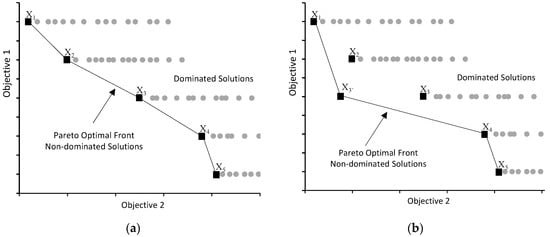
Figure 1.
Pareto Optimal Front. (a) Initial; (b) Updated.
In the present paper, both in the phase of construction and in the phase of the LNS algorithm, every obtained solution is checked for belonging either to the dominated or the non-dominated solutions, as shown in Figure 1a. If a solution obtained from the algorithm belongs to the non-dominated solutions, then the Pareto optimal front is updated. More specifically, in each iteration of the MOLNS, the set of optimal solutions (X1, X2, X3, X4, X5), that belong in the initial Pareto optimal front are selected, as presented in Figure 1a. In case solution X3’ is obtained after the implementation of the removal and insertion operators of the proposed MOLNS algorithm, which improves the value of Objective 2 compared to solution X3, and the values of both Objective 1 and Objective 2 compared to solution X2, the Pareto optimal front must be updated, as shown in Figure 1b. Therefore, every solution obtained from the proposed algorithm is compared to the non-dominated solutions in order to ensure that optimal solutions are maintained and continuously updated.
3.2. Time-Oriented Nearest Neighbor Algorithm
Several heuristic algorithms have been developed for obtaining solutions for the VRP. In the present paper, the Time-Oriented Nearest Neighbor (TONN) algorithm is selected for obtaining the initial solutions, due to its simplicity and speed. The algorithm works by building routes which start from the depot (Node 0) and, consequently, the “closest” to the last visited node unrouted customer is added. In the process of searching the “closest” customer, time window as well as capacity constraints must be respected; otherwise, no customer can be added. A new route is started if no customer is found, unless no more customers are left to add, meaning that all routes have been constructed and the process is completed. Solomon [18] proposed this method in an attempt to optimally solve the VRPTW.
The “closeness” of each customer is measured through metric . This metric measures the direct distance between the two customers , the time difference between the completion of service at i and the beginning of service at j, , and the urgency of delivery to customer j, .
3.3. Multiobjective Large Neighborhood Search
As described in Section 3.2, customers are added in each route based on their “closeness” to the last added customer. However, time windows affect to a great extent the initial solution, which in many cases deviates from the optimum. Therefore, after the initial solutions are constructed, the MOLNS algorithm, which partially destroys and then repairs the solution, is applied for simultaneously minimizing both the number of vehicles and the total distance traveled. The general framework of the LNS algorithm was designed by Ropke and Pisinger [20]. The removal and insertion moves are thoroughly analyzed in Section 3.3.1 and Section 3.3.2.
3.3.1. Removal Operators
In this section, five different removal operators are described for selecting the customers which will be removed from their routes. Most operators are adapted from Ropke and Pisinger [20] and Demir et al. [29], while a new one (distant and waiting-time removal) is presented. From all removal operators, we manage to select s customers and remove them from their routes.
Route Removal
The specific operator removes an entire route from the solution. In each iteration, the route is randomly selected and “destroyed” from the solution. In a later phase, and since all customers must be served, the customers of the “destroyed” route are reinserted according to the insertion operator.
Random Customers Removal
In this operator, a specific number of customers (s) that will be removed from the existing solution is initially determined. Consequently, an empty list of size s is created and filled with customers who are randomly selected. The random nature of this operator increases the diversity, as well as the searching space. As shown in Figure 2, three customers are randomly selected (s = 3) and removed from the route that each one belongs.
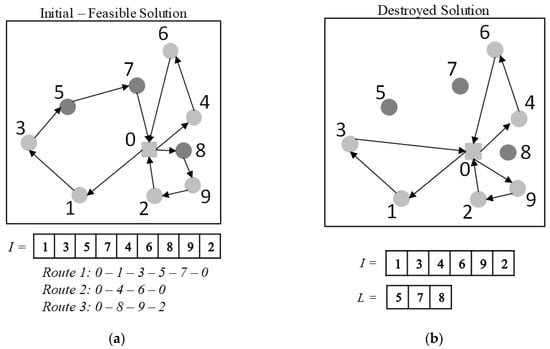
Figure 2.
Removal operator. (a) Initial Solution; (b) “Destroyed” Solution.
Distant Customers Removal
In this operator, as with the case of random customers removal, the number of customers (s) that will be removed from the solution is determined. Consequently, for each customer k, we calculate the metric , where i is the previous delivered customer and j is the next delivered customer, according to k, while d indicates the distance between two customers. We then sort all customers according to the metric ck and select the s “worst” customers (highest ).
Waiting-Time Removal
For each customer to be served, the metric calculates the difference between the start of the time window and the time of arrival. More specifically, the metric for customer i is calculated by , where is the time of arrival at customer i. Consequently, customers are sorted according to metric and s number of customers that have the highest waiting times () are selected.
Distant and Waiting-Time Removal
This operator combines in a single metric both the distant customers removal and the waiting-time removal operators, by assigning weights to both metrics. Similar to the previous operators, a specific number of customers (s) with the worst metrics is selected.
Regardless of the removal operator, the initial solution is presented as an I list containing all customers. The sequence of the elements of I determines the order of customer visitations. When a constraint is violated (capacity or time window), then a new route begins, as shown in Figure 2a. In addition, after the removal operator is applied, the customers that no longer belong to the route are saved in another list L, as shown in Figure 2b.
3.3.2. Insertion Operators
After a removal operator has been applied, an insertion operator must be implemented so that all customers are reinserted in the solution. In the VRPTW, there is a necessary precondition to serve all customers’ needs. In the present paper, three insertion operators are applied and analyzed for improving the initial constructed solution.
Closer Customer Insertion
This operator cooperates with all removal operators. The selected customers of list L are reinserted in the routes and more specifically in the sequence of deliveries where the total distance traveled is minimized. The specific insertion procedure is separated into two different operators. The first one searches for the minimum distance while the number of vehicles must remain the same as before the removal operator was applied. The second operator searches for the minimum distance regardless of the number of vehicles.
Insertion for Minimizing the Number of Vehicles
The specific insertion operator is combined only with the route removal operator in order to decrease the number of vehicles. If all customers of the selected route can be inserted in the rest of the routes, then the number of vehicles is reduced by one, as shown in Figure 3. Simultaneously, we seek to find the best sequence and schedule of deliveries in order to manage the distance traveled as well. However, the fact that VRPTW is a multi-objective optimization problem does not guarantee us that both the number of vehicles and the total distance traveled are simultaneously minimized. Instead, decreasing the number of vehicles by reinserting “destroyed” customers in the best-fitted sequence of deliveries may cause increased total distance traveled. Figure 3 describes how the route removal operator is combined with the specific insertion operator. More specifically, among Routes 1 {0 → i- → i → i+ → 0}, 2 {0 → n → m → 0} and 3 {0 → j- → j → j+ → 0}, the second one (Route 2) is randomly selected and “destroyed”. In the search for inserting customers n and m in the rest of the routes, we form Routes 1’ {0 → i- → m → i → i+ → 0} and 3’ {0 → j- → n → j → j+ → 0}.
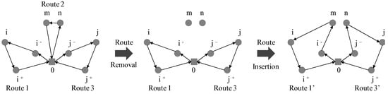
Figure 3.
Route Removal and Reinsertion of Customers.
When implementing the removal and insertion operators, it is essential to ensure the diversity of searching and the global search capabilities. Therefore, after saving the removed customers in list L, as described in Section 3.3.1, the sequence of insertion must be considered. Repeating the same sequence of customers insertion may lead to getting stuck in a local optimum. In the presented insertion operators, a random order for inserting customers is produced, for increasing the search space of the algorithm.
3.3.3. General Framework
Initially, the Pareto optimal solutions constructed from the TONN algorithm are utilized as an input to the MOLNS algorithm, as described in Figure 4. In each iteration that the MOLNS algorithm is implemented, the “removal” and “insertion” operators are applied in each one of the Pareto optimal solutions. Consequently, for each solution, a new one (Xnew) is obtained. If Xnew solution constitutes a Pareto optimal solution, as it belongs to the non-dominated solutions, then the Pareto optimal front is renewed; otherwise, no changes are made.
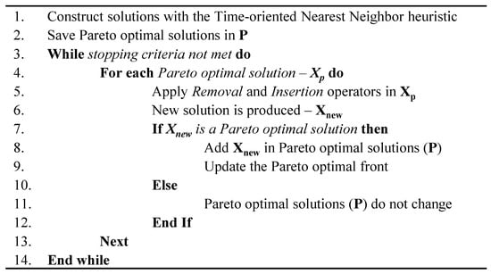
Figure 4.
The general framework of the MOLNS.
4. Experimental Results and Discussion
4.1. Comparisons with Best Known Results
This section describes computational experiments carried out to evaluate the performance of the proposed algorithm. The algorithm was coded in Python and ran on a personal computer with the following specifications: Intel Core i7 (Intel Corporation, California, USA)—8550U 1.8 GHz with 16 GB memory. The proposed algorithm was tested in Solomon’s VRPTW benchmark instances with 100 customers (see [18]), as well as in Gehring and Homberger’s instances with 1000 customers (see [30]). In the specific datasets, C1 and C2 problems have geographically clustered customers; in R1 and R2, geographical data are randomly generated; and in RC1 and RC2, a mix of random and clustered structures is included. R1, C1 and RC1 have a short scheduling horizon, narrow time windows and low vehicle capacities, respectively, while R2, C2 and RC2 have a long scheduling horizon, wide time windows and high vehicle capacities, defining the number of customers serviced by the same vehicle.
Table 1 and Table 2 present a summary of the results obtained from our proposed MOLNS algorithm in Solomon’s instances, as well as the best-published solutions in the literature. The column labeled BP gives the best-published results, while column MOLNS the results of our Large Neighborhood Search algorithm. Each solution is characterized by the number of vehicles (NV) needed and the total distance traveled (TD). The published work in which the optimum solution is proposed is presented in column “Reference”, the computational time needed to obtain each solution is given in column “Time” in seconds and the percentage deviation in the total distance traveled between the BP and the LNS is presented in column “Deviation”.

Table 1.
Solomon instances with short scheduling horizon: comparison of our MOLNS with the best-published results.
Table 2.
Solomon instances with long scheduling horizon: comparison of our MOLNS with the best-published results.
Each instance was run three times, while the computational time limit was set to be 5 min, which is a reasonable time for a logistics company to obtain the routing of their vehicles and the scheduling of their deliveries. In most cases, the best-obtained results needed less time than the time limit. Since we face the multiobjective VRPTW in some instances, more than one solution was obtained. In order for the BP solution and the solution obtained from the MOLNS to be comparable, the number of vehicles must be the same. Therefore, the deviation is measured in the total distance traveled between the BP solution and the solution of the MOLNS. It can be easily observed that instances with geographically clustered customers (C1 and C2) have more efficient results than problems with random geographical data, as the mean deviation in that case is 0.30%. In randomly generated geographical data (R), the mean deviation is higher and reaches 3.37%, while in mixed geographical customers’ data (RC) it is 3.47%. Finally, the mean deviation for all instances is less than 2.85%, which can be considered very efficient, since the optimal results have emerged from multiple researchers over time. In total, 32.47% of the comparable solutions have a deviation of less than 1%, most of them in C instances. Simultaneously, 98.70% of the results deviate less than 10% from the optimum. Finally, three new Pareto-optimal solutions are proposed in Solomon’s benchmark instances, in RC202, RC207 and R201. In RC202 problem, a decrease in the total distance traveled is accomplished, but at the expense of an increased number of vehicles. In R201 and RC202 instances, we managed to improve the solutions by decreasing the total distance traveled, while the number of vehicles remains steady. The exact routes and the schedule of deliveries in each of the three new optimal solutions that are proposed in the current research are given in Appendix A.
Additionally, when comparing results obtained from algorithms, it is important to take into consideration the computational time needed. Chiang and Hsu [24] managed to produce high-quality solutions within 0.5 min and thoroughly presented data related to the computational time for other algorithms addressing this problem. Ghoseiri and Ghannadpour [31] and Ombuki et al. [23], who also considered the VRPTW as multiobjective, did not present the computational time needed, while the proposed algorithm manages to produce high efficiency results in less than a minute (52 s on average). Of course, the CPU as well as the programming language are also important factors affecting the computational time needed.
Finally, in Gehring and Homberger’s benchmark instances, the number of customers vary from 200 to 1000. In the current research, the algorithm was tested in instances with 1000 customers in order to identify its efficiency in terms of quality of results and computational time, when the number of customers is extremely high. These instances, as in the case of Solomon’s, are categorized into six cases: C1, C2, R1, R2, RC1 and RC2. In Table 3, the average number of vehicle as well as the average traveled distance, of both the best-published (BP) solutions and the solutions produced by the MOLNS algorithm, are presented for each case. In addition, the percentage deviation between the solutions was calculated for each objective (deviation in the NV and deviation in the TD). More specifically, the mean deviation for all cases concerning the number of vehicles is 6.63%, and 10.60% for the traveled distance. On the contrary, the corresponding percentage in the TD in Solomon’s instances is 2.85%, indicating that the quality of results is affected to a small extent when the number of customers increases. However, the mean computational time needed (Time column) for each case to be solved remains reasonable and low, given the volume of customers.
Table 3.
Gehring and Homberger’s instances with 1000 customers: comparison of our MOLNS with the best-published results.
4.2. Discussion on Real-Life Implementation of the Algorithm
Every algorithm presents specific advantages and disadvantages. However, regardless of the algorithm, when multiple VRP variants are involved in the optimization process, the computation time is increased. Heuristic algorithms used to be applied and implemented in routing and scheduling software, due to their ability to perform in a relatively limited search space and simultaneously produce efficient solutions in limited computing time [51]. On the other hand, metaheuristic algorithms operate a wider search space, but this does not necessarily mean that the computational time will significantly increase. The advances of technology and computer science give researchers the ability to produce near-optimal solutions, and in most cases better than those produced by heuristics. Therefore, metaheuristics should be considered for implementation in routing software solutions due to offering reliable and on-time deliveries to transportation companies.
Gayialis et al. [52], Rincon-Garcia et al. [53] and Veres et al. [54] described the design and requirements of various routing and scheduling software that need fast and efficient solutions both for the initial planning and for the rescheduling of deliveries. It is clear that practitioners and companies are looking for efficient algorithms to integrate into their software solutions for logistics operations. According to Table 1, Table 2 and Table 3, the proposed MOLNS algorithm offers near-optimal solutions in a reasonable time, while also having the ability to solve cases with a higher number of customers and rendering the algorithm ideal for the routing of vehicles and scheduling of deliveries in real-life cases. Therefore, the proposed algorithm can be implemented in a software solution, to solve the problem of routing and scheduling of deliveries effectively. That was the scope of the developed algorithm from the beginning and the current research proves that it is in line with this scope.
As noted in the Introduction, information available to the planner commonly changes in real-life cases after the completion of the initial routing and scheduling. Consequently, a rapid rescheduling procedure that is fed with dynamic data becomes a necessity to create a viable real-life routing and rescheduling system. This becomes even more clear when considering that, in real-life cases, changes may even occur while vehicles are on the road to deliver the orders, and, therefore, rapid rescheduling becomes mandatory. The algorithm presented in this paper can also support the dynamic aspect of the VRPTW, as the removal and insertion operators of the MOLNS algorithm can handle changes of the input data, such as travel times between nodes. Hence, the algorithm can be applied for both the initial plan and the rescheduling procedure by applying some minor modifications.
5. Conclusions and Further Research
The results obtained from the MOLNS algorithm were compared to both the best-published solutions in Solomon’s dataset, as well as to those of other multiobjective algorithms, providing us significant insights about this method. Based on the conducted research, as it becomes clear, no algorithm can obtain all Pareto optimal solutions in each instance in Solomon’s dataset. Instead, the results have been conjunctly obtained from multiple algorithms since the VRPTW first appeared. The results of the proposed MOLNS algorithm are near-optimal, with only small deviations from the optimal, and even include three new non-dominated solutions. The computational experiments indicate that the results are efficient and are obtained in a very realistic time. As both efficiency and speed are critical factors when implementing an algorithm in software solutions, the proposed MOLNS algorithm can be examined for implementation in such software, and this will in fact be the next step of our research.
In real-life scenarios, performing an initial plan of routes and deliveries does not necessarily fulfill the purpose of distribution services. Unforeseen events and traffic congestion, in many cases and especially in the urban environment, cause delays and generate the need for rescheduling, in order to ensure that all deliveries are executed and served on-time. The presented algorithm can be easily adapted and applied in dynamic routing cases to calculate new schedules of deliveries efficiently and quickly. The implementation of the proposed algorithm in a software solution for logistics operations, therefore, needs to be further researched. Additionally, the potential reinforcement of the algorithm to solve cases that require the dynamic rescheduling of deliveries should also be studied. Recent advances in technology, such as traffic management sensors, real-time traffic data and the Internet of things technology, can provide data to enhance such rescheduling procedures and deal with the dynamic nature of the real-life problems. In addition, the algorithm could be further enhanced by applying multicriteria decision making approaches such as the one presented by Kechagias et al. [55] to optimize its function in accordance with different use-case scenarios. Finally, provided the aforementioned technologies are successfully combined with the proposed algorithm, in the next step of our research, an advanced software solution that can support the distribution processes of logistics companies, in the urban environment, while, at the same time, focusing on the fulfillment of time-window restrictions, will be created.
Author Contributions
Conceptualization, G.D.K. and S.P.G.; methodology, G.D.K. and E.P.K.; software, G.D.K. and E.P.K.; validation, G.D.K, S.P.G and E.P.K.; formal analysis, G.D.K.; investigation, G.D.K. and E.P.K.; resources, S.P.G., G.A.P. and I.P.T.; data curation, G.D.K.; writing—original draft preparation, G.D.K and S.P.G.; writing—review and editing, G.D.K, S.P.G, E.P.K. and I.P.T.; visualization, G.D.K and G.A.P.; supervision, S.P.G., I.P.T. and G.A.P.; project administration, S.P.G. and I.P.T.; and funding acquisition, S.P.G., I.P.T. and G.A.P. All authors have read and agreed to the published version of the manuscript.
Funding
The present work was co-funded by the European Union and Greek national funds through the Operational Program “Competitiveness, Entrepreneurship and Innovation” (EPAnEK), under the call “RESEARCH-CREATEINNOVATE” (Project Code: T1EDK-00527 and Acronym: SMARTRANS).
Acknowledgments
In this section you can acknowledge any support given which is not covered by the author contribution or funding sections. This may include administrative and technical support, or donations in kind (e.g., materials used for experiments).
Conflicts of Interest
The authors declare no conflict of interest.
Appendix A
Solutions in Solomon’s instances which improve the results and offer new Pareto-optimal solutions are given below:
Appendix A.1. RC202: Number of Vehicles = 7, Total Distance Traveled = 1117.41
- Route 1: 0 → 65 - 83 → 64 → 23 → 21 → 48 → 18 → 19 → 49 → 22 → 20 → 24 → 25 → 77 → 75 → 58 → 52 → 82 → 0
- Route 2: 0 → 69 → 68 → 88 → 53 → 99 → 57 → 86 → 87 → 9 → 10 → 97 → 59 → 74 → 13 → 17 → 60 → 100 → 70 → 0
- Route 3: 0 → 14 → 47 → 16 → 15 → 11 → 12 → 78 → 73 → 79 → 7 → 6 → 8 → 46 → 4 → 2 → 55 → 0
- Route 4: 0 → 71 → 67 → 62 → 76 → 51 → 84 → 56 → 66 → 0
- Route 5: 0 → 92 → 95 → 85 → 63 → 33 → 34 → 31 → 29 → 27 → 26 → 28 → 30 → 32 → 89 → 50 → 93 → 96 → 94 → 91 → 80 → 0
- Route 6: 0 → 45 → 5 → 3 → 1 → 42 → 39 → 37 → 36 → 44 → 41 → 38 → 40 → 43 → 35 → 72 → 54 → 68 → 0
- Route 7: 0 → 81 → 61 → 90 → 0
Appendix A.2. RC207: Number of Vehicles = 5, Total Distance Traveled = 970.78
- Route 1: 0 → 92 → 95 → 67 → 31 → 29 → 28 → 30 → 63 → 85 → 76 → 18 → 21 → 23 → 19 → 49 → 22 → 51 → 84 → 62 → 50 → 34 → 27 → 26 → 32 → 33 → 89 → 56 → 91 → 80 → 0
- Route 2: 0 → 69 → 98 → 88 → 78 → 73 → 79 → 7 → 6 → 2 → 8 → 5 → 3 → 1 → 45 → 4 → 46 → 60 → 55 → 100 → 70 → 68 → 0
- Route 3: 0 → 61 → 72 → 71 → 93 → 94 → 81 → 42 → 44 → 40 → 36 → 35 → 37 → 38 → 39 → 43 → 41 → 54 → 96 → 0
- Route 4: 0 → 64 → 83 → 99 → 52 → 86 → 75 → 59 → 87 → 74 → 57 → 65 → 90 → 0
- Route 5: 0 → 82 → 53 → 12 → 14 → 47 → 17 → 16 → 15 → 11 → 10 → 9 → 13 → 97 → 58 → 77 → 25 → 48 → 20 → 24 → 66 → 0
Appendix A.3. R201: Number of Vehicles = 7, Total Distance Traveled = 1156.73
- Route 1: 0 → 5 → 83 → 45 → 82 → 47 → 36 → 19 → 11 → 64 → 49 → 46 → 48 → 0
- Route 2: 0 → 95 → 59 → 92 → 42 → 15 → 14 → 98 → 61 → 16 → 44 → 38 → 86 → 85 → 99 → 6 → 94 → 53 → 26 → 0
- Route 3: 0 → 28 → 12 → 29 → 76 → 21 → 73 → 40 → 87 → 57 → 43 → 37 → 97 → 96 → 13 → 58 → 0
- Route 4: 0 → 33 → 65 → 71 → 30 → 51 → 9 → 81 → 79 → 78 → 34 → 50 → 3 → 68 → 54 → 0
- Route 5: 0 → 2 → 72 → 39 → 67 → 23 → 75 → 22 → 41 → 56 → 74 → 4 → 55 → 25 → 24 → 80 → 77 → 0
- Route 6: 0 → 52 → 69 → 31 → 88 → 7 → 18 → 8 → 84 → 17 → 91 → 100 → 93 → 60 → 89 → 0
- Route 7: 0 → 27 → 62 → 63 → 90 → 10 → 20 → 66 → 35 → 32 → 70 → 1 → 0
References
- Dantzig, G.B.; Ramser, J.H. The truck dispatching problem. Manag. Sci. 1959, 6. [Google Scholar] [CrossRef]
- Lin, C.; Choy, K.L.; Ho, G.T.S.; Chung, S.H.; Lam, H.Y. Survey of Green Vehicle Routing Problem: Past and future trends. Expert Syst. Appl. 2014, 41, 1118–1138. [Google Scholar] [CrossRef]
- Konstantakopoulos, G.D.; Gayialis, S.P.; Kechagias, E.P. Vehicle routing problem and related algorithms for logistics distribution: A literature review and classification. Oper. Res. Int. J. 2020. [Google Scholar] [CrossRef]
- Juárez Pérez, M.; Pérez Loaiza, R.E.; Quintero Flores, P.M.; Atriano Ponce, O.; Flores Peralta, C. A Heuristic Algorithm for the Routing and Scheduling Problem with Time Windows: A Case Study of the Automotive Industry in Mexico. Algorithms 2019, 12, 111. [Google Scholar] [CrossRef]
- Nagata, Y.; Bräysy, O.; Dullaert, W. A penalty-based edge assembly memetic algorithm for the vehicle routing problem with time windows. Comput. Oper. Res. 2010, 37, 724–737. [Google Scholar] [CrossRef]
- Ait Haddadene, S.; Labadie, N.; Prodhon, C. Bicriteria Vehicle Routing Problem with Preferences and Timing Constraints in Home Health Care Services. Algorithms 2019, 12, 152. [Google Scholar] [CrossRef]
- Taş, D.; Jabali, O.; Van Woensel, T. A vehicle routing problem with flexible time windows. Comput. Oper. Res. 2014, 52, 39–54. [Google Scholar] [CrossRef]
- Taillard, E.; Badeau, P.; Gendreau, M.; Guertin, F.; Potvin, J.-Y. A Tabu Search Heuristic for the Vehicle Routing Problem with Soft Time Windows. Transp. Sci. 1997, 31, 170–186. [Google Scholar] [CrossRef]
- Iqbal, S.; Rahman, M.S. Vehicle routing problems with soft time windows. In Proceedings of the 2012 7th International Conference on Electrical and Computer Engineering, Dhaka, Bangladesh, 20–22 December 2012; pp. 634–638. [Google Scholar]
- Wu, L.; He, Z.; Chen, Y.; Wu, D.; Cui, J. Brainstorming-Based Ant Colony Optimization for Vehicle Routing with Soft Time Windows. IEEE Access 2019, 7, 19643–19652. [Google Scholar] [CrossRef]
- Hashimoto, H.; Ibaraki, T.; Imahori, S.; Yagiura, M. The vehicle routing problem with flexible time windows and traveling times. Discret. Appl. Math. 2006, 154, 2271–2290. [Google Scholar] [CrossRef][Green Version]
- Koskosidis, Y.A.; Powell, W.B.; Solomon, M.M. An optimization-based heuristic for vehicle routing and scheduling with soft time window constraints. Transp. Sci. 1992, 26, 69–85. [Google Scholar] [CrossRef]
- Arnold, F.; Sörensen, K. What makes a VRP solution good? The generation of problem-specific knowledge for heuristics. Comput. Oper. Res. 2019, 106, 280–288. [Google Scholar] [CrossRef]
- Ibaraki, T.; Kubo, M.; Masuda, T.; Uno, T.; Yagiura, M. Effective local search algorithms for the vehicle routing problem with general time window constraints. In Proceedings of the MIC, Porto, Portugal, 16–20 July 2001. [Google Scholar]
- Kalayci, C.B.; Kaya, C. An ant colony system empowered variable neighborhood search algorithm for the vehicle routing problem with simultaneous pickup and delivery. Expert Syst. Appl. 2016, 66, 163–175. [Google Scholar] [CrossRef]
- El-Sherbeny, N.A. Vehicle routing with time windows: An overview of exact, heuristic and metaheuristic methods. J. King Saud Univ. Sci. 2010, 22, 123–131. [Google Scholar] [CrossRef]
- Bräysy, O.; Gendreau, M. Vehicle Routing Problem with Time Windows, Part I: Route Construction and Local Search Algorithms. Transp. Sci. 2005, 39, 104–118. [Google Scholar] [CrossRef]
- Solomon, M.M. Algorithms for the vehicle routing and scheduling problems with time window constraints. Oper. Res. 1987, 35, 254–265. [Google Scholar] [CrossRef]
- Shaw, P. Using Constraint Programming and Local Search Methods to Solve Vehicle Routing Problems. In Principles and Practice of Constraint Programming—CP98, Proceedings of the International Conference on Principles and Practice of Constraint Programming, Pisa, Italy, 26–30 October 1998; Maher, M., Puget, J.-F., Eds.; Springer: Berlin/Heidelberg, Germany, 1998; pp. 417–431. [Google Scholar]
- Ropke, S.; Pisinger, D. An Adaptive Large Neighborhood Search Heuristic for the Pickup and Delivery Problem with Time Windows. Transp. Sci. 2006, 40, 455–472. [Google Scholar] [CrossRef]
- Konak, A.; Coit, D.W.; Smith, A.E. Multi-objective optimization using genetic algorithms: A tutorial. Reliab. Eng. Syst. Saf. 2006, 91, 992–1007. [Google Scholar] [CrossRef]
- Tan, K.C.; Chew, Y.H.; Lee, L.H. A Hybrid Multiobjective Evolutionary Algorithm for Solving Vehicle Routing Problem. Comput. Optim. Appl. 2006, 34, 115–151. [Google Scholar] [CrossRef]
- Ombuki, B.; Ross, B.J.; Hanshar, F. Multi-objective genetic algorithms for vehicle routing problem with time windows. Appl. Intell. 2006, 24, 17–30. [Google Scholar] [CrossRef]
- Chiang, T.C.; Hsu, W.H. A knowledge-based evolutionary algorithm for the multiobjective vehicle routing problem with time windows. Comput. Oper. Res. 2014, 45, 25–37. [Google Scholar] [CrossRef]
- Garcia-Najera, A.; Bullinaria, J.A. An improved multi-objective evolutionary algorithm for the vehicle routing problem with time windows. Comput. Oper. Res. 2011, 38, 287–300. [Google Scholar] [CrossRef]
- Baños, R.; Ortega, J.; Gil, C.; Márquez, A.L.; De Toro, F. A hybrid meta-heuristic for multi-objective Vehicle Routing Problems with Time Windows. Comput. Ind. Eng. 2013, 65, 286–296. [Google Scholar] [CrossRef]
- Yun, Y.; Nakayama, H.; Yoon, M. Generation of Pareto optimal solutions using generalized DEA and PSO. J. Glob. Optim. 2016, 64, 49–61. [Google Scholar] [CrossRef]
- Ehrgott, M. Multicriteria Optimization, 2nd ed.; Springer Science & Business Media: Berlin/Heidelberg, Germany, 2005. [Google Scholar]
- Demir, E.; Bektaş, T.; Laporte, G. An adaptive large neighborhood search heuristic for the Pollution-Routing Problem. Eur. J. Oper. Res. 2012, 223, 346–359. [Google Scholar] [CrossRef]
- Transportation Optimization Portal/VRPTW. Available online: https://www.sintef.no/projectweb/top/vrptw/homberger-benchmark/ (accessed on 18 September 2020).
- Ghoseiri, K.; Ghannadpour, S.F. Multi-objective vehicle routing problem with time windows using goal programming and genetic algorithm. Appl. Soft Comput. 2010, 10, 1096–1107. [Google Scholar] [CrossRef]
- Desrochers, M.; Desrosiers, J.; Solomon, M. A new optimization algorithm for the vehicle routing problem with time windows. Oper. Res. 1992, 40, 342–354. [Google Scholar] [CrossRef]
- Tavares, J.; Pereira, F.B.; Machado, P.; Costa, E. On the influence of GVR in vehicle routing. In Proceedings of the SAC, Melbourne, FL, USA, 9–12 March 2003; Volume 3, pp. 753–758. [Google Scholar]
- Lau, H.C.; Lim, Y.F.; Liu, Q.Z. Diversification of search neighborhood via constraint-based local search and its applications to VRPTW. In Proceedings of the 3rd International Workshop on Integration of AI and OR Techniques (CP-AI-OR), Kent, UK, 8–10 April 2001; pp. 1–15. [Google Scholar]
- Kallehauge, B.; Larsen, J.; Madsen, O.B.G. Lagrangean duality applied on vehicle routing with time windows. Comput. Oper. Res. 2006, 33, 1464–1487. [Google Scholar] [CrossRef]
- Cook, W.; Rich, J.L. A Parallel Cutting-Plane Algorithm for the Vehicle Routing Problem with Time Windows; Rice University: Houston, TX, USA, 1999. [Google Scholar]
- Yu, B.; Yang, Z.Z.; Yao, B.Z. A hybrid algorithm for vehicle routing problem with time windows. Expert Syst. Appl. 2011, 38, 435–441. [Google Scholar] [CrossRef]
- Rochat, Y.; Taillard, É.D. Probabilistic diversification and intensification in local search for vehicle routing. J. Heuristics 1995, 1, 147–167. [Google Scholar] [CrossRef]
- Kohl, N.; Desrosiers, J.; Madsen, O.B.G.; Solomon, M.M.; Soumis, F. 2-Path Cuts for the Vehicle Routing Problem with Time Windows. Transp. Sci. 1999, 33. [Google Scholar] [CrossRef]
- Shaw, P. A New Local Search Algorithm Providing High Quality Solutions to Vehicle Routing Problems. Available online: http://citeseerx.ist.psu.edu/viewdoc/download?doi=10.1.1.51.1273&rep=rep1&type=pdf (accessed on 25 September 2020).
- Alvarenga, G.B.; Mateus, G.R.; de Tomi, G. A genetic and set partitioning two-phase approach for the vehicle routing problem with time windows. Comput. Oper. Res. 2007, 34, 1561–1584. [Google Scholar] [CrossRef]
- Li, H.; Lim, A. Local search with annealing-like restarts to solve the VRPTW. Eur. J. Oper. Res. 2003, 150, 115–127. [Google Scholar] [CrossRef]
- Potvin, J.Y.; Bengio, S. The Vehicle Routing Problem with Time Windows Part II: Genetic Search. INFORMS J. Comput. 1996, 8, 165–172. [Google Scholar] [CrossRef]
- Homberger, J.; Gehring, H. Two evolutionary metaheuristics for the vehicle routing problem with time windows. INFOR Inf. Syst. Oper. Res. 1999, 37, 297–318. [Google Scholar] [CrossRef]
- Rousseau, L.-M.; Gendreau, M.; Pesant, G. Using constraint-based operators to solve the vehicle routing problem with time windows. J. Heuristics 2002, 8, 43–58. [Google Scholar] [CrossRef]
- Thangiah, S.R.; Osman, I.H.; Sun, T. Hybrid Genetic Algorithm, Simulated Annealing and Tabu Search Methods for Vehicle Routing Problems with Time Windows; Technical Report No. SRU CpSc-TR-94-27; Computer Science Department, Slippery Rock University: Slippery Rock, PA, USA, 1994; Volume 69. [Google Scholar]
- Labadi, N.; Prins, C.; Reghioui, M. A memetic algorithm for the vehicle routing problem with time windows. RAIRO-Operations Res. 2008, 42, 415–431. [Google Scholar] [CrossRef]
- Mester, D.; Bräysy, O.; Dullaert, W. A multi-parametric evolution strategies algorithm for vehicle routing problems. Expert Syst. Appl. 2007, 32, 508–517. [Google Scholar] [CrossRef]
- Barbucha, D. A cooperative population learning algorithm for vehicle routing problem with time windows. Neurocomputing 2014, 146, 210–229. [Google Scholar] [CrossRef]
- de Oliveira, H.C.; Vasconcelos, G.C. A hybrid search method for the vehicle routing problem with time windows. Ann. Oper. Res. 2010, 180, 125–144. [Google Scholar]
- Gayialis, S.P.; Tatsiopoulos, I.P. Design of an IT-driven decision support system for vehicle routing and scheduling. Eur. J. Oper. Res. 2004, 152, 382–398. [Google Scholar] [CrossRef]
- Gayialis, S.P.; Konstantakopoulos, G.D.; Papadopoulos, G.A.; Kechagias, E.; Ponis, S.T. Developing an Advanced Cloud-Based Vehicle Routing and Scheduling System for Urban Freight Transportation. In Proceedings of the IFIP International Conference on Advances in Production Management Systems, Seoul, Korea, 26–30 August 2018; pp. 190–197. [Google Scholar]
- Rincon-Garcia, N.; Waterson, B.J.; Cherrett, T.J. Requirements from vehicle routing software: Perspectives from literature, developers and the freight industry. Transp. Rev. 2018, 38, 117–138. [Google Scholar] [CrossRef]
- Veres, P.; Bányai, T.; Illés, B. Intelligent Transportation Systems to Support Production Logistics. In Proceedings of the Vehicle and Automotive Engineering; Jármai, K., Bolló, B., Eds.; Springer International Publishing: Cham, Switzerland, 2017; pp. 245–256. [Google Scholar]
- Kechagias, E.P.; Gayialis, S.P.; Konstantakopoulos, G.D.; Papadopoulos, G.A. An Application of a Multi-Criteria Approach for the Development of a Process Reference Model for Supply Chain Operations. Sustainability 2020, 12, 5791. [Google Scholar] [CrossRef]


© 2020 by the authors. Licensee MDPI, Basel, Switzerland. This article is an open access article distributed under the terms and conditions of the Creative Commons Attribution (CC BY) license (http://creativecommons.org/licenses/by/4.0/).