1. Introduction
The goal of graph partitioning is to divide a graph into a given number of roughly equally sized parts by removing a small number of edges or nodes. Graph partitioning has many practical applications, such as accelerating matrix multiplication, dividing compute workloads, image processing, circuit design, and the focus of this work, accelerating shortest path computations in road networks. For an overview of the state-of-the-art in graph partitioning, we refer the reader to a survey article [
1].
Computing shortest paths in road networks is a fundamental building block in applications such as navigation systems (e.g., Google Maps), logistics planning, and traffic simulation. Unfortunately, Dijkstra’s algorithm [
2] takes over a second for a single query on continental-size road networks with tens of millions of nodes, rendering it infeasible for interactive scenarios. This has led to a large amount of research on speedup techniques [
3], which often use an expensive preprocessing phase to enable fast queries. Arc-Flags [
4,
5] is one of the early techniques that use graph partitioning. It has been frequently used to enhance other techniques, e.g., SHARC [
6], combining shortcuts [
7] and Arc-Flags, ReachFlags [
8], combining Reach [
9] and Arc-Flags as well as CHASE [
8], combining Contraction Hierarchies [
10] and Arc-Flags. In navigation systems, the graph topology changes infrequently, but the metric (arc weights) changes frequently, e.g., due to traffic congestion or road closures. To accommodate this, modern speedup techniques split the preprocessing phase into an expensive metric-independent preprocessing phase and a fast metric-dependent
customization phase. The two state-of-the-art techniques are Multilevel Overlays, also known as Customizable Route Planning [
11], which use nested k-way partitions and Customizable Contraction Hierarchies (CCHs) [
12], which use nested dissection orders [
13]. In this work, we focus on CCHs, which extend classic two-phase Contraction Hierarchies [
10] to the three-phase approach with customization.
Contraction Hierarchies simulate contracting all nodes in a given order and insert shortcut arcs between the neighbors of a contracted node. These represent paths via the contracted nodes. Shortest
s–
t path queries are answered by, e.g., a bidirectional Dijkstra search [
2] from
s and
t, which only considers shortcut and original arcs to higher-ranked nodes. Thus, nodes which lie on many shortest paths should be ranked high in the order. Customizable Contraction Hierarchies [
12] use contraction orders computed via recursive balanced node separators (nested dissection) in order to achieve a logarithmic search space depth with few added shortcuts. Node separators are considered to lie on many shortest paths, as any path between the components crosses the separator. The weights of the contraction hierarchy can then be quickly customized to any metric, allowing, e.g., the incorporation of real-time traffic information. The running time needed for the customization and the shortest path queries depends on the quality of the calculated order. Previously proposed partitioning tools for computing separators in road networks include FlowCutter [
14], Inertial Flow [
15], KaHiP [
16], Metis [
17], PUNCH [
18], and Buffoon [
19]. KaHiP and Metis are general-purpose graph partitioning tools. PUNCH and Buffoon are special-purpose partitioners, which aim to use geographical features of road networks such as rivers or mountains. Rivers and mountains form very small cuts and were dubbed
natural cuts in [
18]. PUNCH identifies and deletes natural cuts, then contracts the remaining components and subsequently runs a variety of highly randomized local search algorithms. Buffoon incorporates the idea of natural cuts into KaHiP, running its evolutionary multilevel partitioner instead of the flat local searches of PUNCH. In [
14], it was shown that FlowCutter is also able to identify and leverage natural cuts. Inertial Flow is another special-purpose partitioner that is even based on using the geographic embedding of the road network.
We combine the idea of Inertial Flow to use geographic coordinates with the incremental cut computations of FlowCutter. This allows us to compute a series of cuts with suitable balances much faster than FlowCutter while still achieving high quality. In an extensive experimental evaluation, we compare our new algorithm InertialFlowCutter to the state-of-the-art. Thus far, FlowCutter has been the best method for computing CCH orders. InertialFlowCutter computes slightly better CCH orders than FlowCutter and is a factor of 5.7 and 6.6 faster on the road networks of the USA and Europe, respectively—our two most relevant instances. Using 16 cores of a shared-memory machine, we can compute CCH orders for these instances in four minutes.
In
Section 2, we briefly present the existing Inertial Flow and FlowCutter algorithms and describe how we combined them. In
Section 3, we describe the setup and results of our experimental study. We conclude with a discussion of our results and future research directions in
Section 4.
This paper recreates the experiments from [
14] and uses a lot of the same setup. Therefore, there is substantial content overlap. To keep this paper self-contained, we repeat the parts we use. Our contributions are the InertialFlowCutter algorithm, an improved Inertial Flow implementation and a reproduction of the experiments from [
14], including InertialFlowCutter and a newer KaHiP version.
2. Materials and Methods
After introducing preliminaries, we describe the existing biparitioning algorithms FlowCutter and Inertial Flow on a high level, before discussing how to combine them into our new algorithm InertialFlowCutter. We refer the interested reader to [
14] for implementation details and a more in-depth discussion of the FlowCutter algorithm. Then, we discuss our application Customizable Contraction Hierarchies (CCH), what makes a good CCH order, and how we use recursive bisection to compute them.
2.1. Preliminaries
An undirected graph consists of a set of nodesV and a set of edges . A directed graph has directed arcs instead of undirected edges. It is symmetric if for every arc , the reverse arc is in A. For ease of notation, we do not distinguish between undirected and symmetric graphs in this paper, and we use them interchangeably, whichever better suits the description. Let denote the number of nodes and let denote the number of edges of an undirected graph. All graphs in this paper contain neither self-loops nor multiedges. is a subgraph of G if and . The subgraph induced by a node set is defined as , the graph with nodes U and all arcs of G with endpoints in U. The degree is the number of outgoing arcs of x. A path is a sequence of edges such that consecutive edges overlap in a node. A graph is called k-connected if there are k node-disjoint paths between every pair of nodes. The k-connected components of a graph are the node-induced subgraphs, which are inclusion-maximal regarding k-connectivity. 1-connected components are called connected components, while 2-connected components are called biconnected components.
2.1.1. Separators and Cuts
Let be a bipartition of into two non-empty disjoint sets, called blocks. The cut induced by is the set of edges between and . The cut size is . We often use the terms cut and bipartition interchangeably. Sometimes, we say a bipartition is induced by a set of cut edges. A node separator partition is a partition of into three disjoint sets such that there is no edge between and . We call Q the separator and the blocks or components of the separator. is the separator size. For an , a cut or separator is -balanced if . We often call the imbalance, as larger values correspond to less balanced cuts. The balanced graph bipartitioning [balanced node separator] problem is to find an -balanced cut [separator] of minimum size. Let be two fixed, disjoint, non-empty subsets of V. An edge cut [node separator] is an S–T edge cut [node separator] if and .
2.1.2. Maximum Flows
A flow network
is a simple symmetric directed graph
with two disjoint non-empty
terminal node sets
, also called the source and target node set, as well as a capacity function
. A flow in
is a function
subject to the
capacity constraint for all arcs
a,
flow conservation for all nonterminal nodes
v, and
skew symmetry for all arcs
. In this paper, we consider only unit flows and unit capacities, i.e.,
,
. The
value of a flow
is the amount of flow leaving
S. The
residual capacity is the additional amount of flow that can pass through
a without violating the capacity constraint. The residual network with respect to
f is the directed graph
, where
. An
augmenting path is an
S–
T path in
. A node
v is called
source-reachable if there is a path from
S to
v in
. We denote the set of source-reachable nodes by
, and define the set of
target-reachable nodes
analogously. The flow
f is a
maximum flow if
is maximal among all possible flows in
. This is the case if and only if there is no augmenting path in
. The well-known max-flow–min-cut theorem [
20] states that the value of a maximum flow equals the capacity of a minimum
S–
T edge cut.
is the source-side cut, and
is the target-side cut of a maximum flow.
2.2. Flowcutter
FlowCutter is an algorithm for the balanced graph bipartitioning problem. The idea of its core algorithm is to solve a sequence of incremental max flow problems, which induce cuts with monotonically increasing cut size and balance, until the latest cut induces an -balanced bipartition. The flow problems are incremental in the sense that the terminal nodes of the previous flow problem are subsets of the terminals in the next flow problem. This nesting allows us to reuse the flow computed in previous iterations.
Given randomly chosen starting terminal nodes , we set and compute a maximum S–T flow. Then, we transform the S-reachable nodes to sources if , or to targets otherwise. Assume without loss of generality. Now S induces a minimum S–T cut . If is -balanced, the algorithm terminates. Otherwise, we transform one additional node, called piercing node, to a source. The piercing node is chosen from the nodes incident to the cut and not in S. This step is called piercing the cut . It ensures that we will find a different cut in the next iteration. Subsequently, we augment the previous flow to a maximum flow that considers the new source node. These steps are repeated until the latest cut induces an -balanced bipartition. Algorithm 1 shows pseudocode for FlowCutter.
| Algorithm 1: FlowCutter |
 |
A significant detail of the piercing step is that piercing nodes which are not reachable from the opposite side are preferred. Choosing such nodes for piercing does not create augmenting paths. Thus, the cut size does not increase in the next iteration. This is called the
avoid-augmenting-paths heuristic. A secondary
distance-based piercing heuristic is used to break ties, when the avoid-augmenting-paths heuristic gives multiple choices. It chooses the node
p which minimizes
, where dist is the hop distance, precomputed via Breadth-First-Search from
s and
t. Roughly speaking, this attempts to prevent the cut sides from meeting before perfect balance. It also has a geometric interpretation, which is explained in [
14].
We choose the starting terminal nodes
s and
t uniformly at random. Experiments [
14] indicate that 20 terminal pairs are sufficient to obtain high quality partitions of road networks.
For computing maximum flows, we use the basic Ford–Fulkerson algorithm [
20], with Pseudo- Depth-First-Search for finding augmenting paths. Pseudo-Depth-First-Search directly marks all adjacent nodes as visited when processing a node. It can be implemented like Breadth-First-Search using a stack instead of a queue.
A major advantage of FlowCutter over other partitioning tools is the fact that it computes multiple cuts. From this set of cuts, we derive the Pareto cutset, which we define as the set of all nondominated cuts. A cut is dominated by a cut if has neither better balance nor smaller cut size than . Instead of selecting a maximum imbalance a priori, we can select a good trade-off between cut size and imbalance from the Pareto cutset.
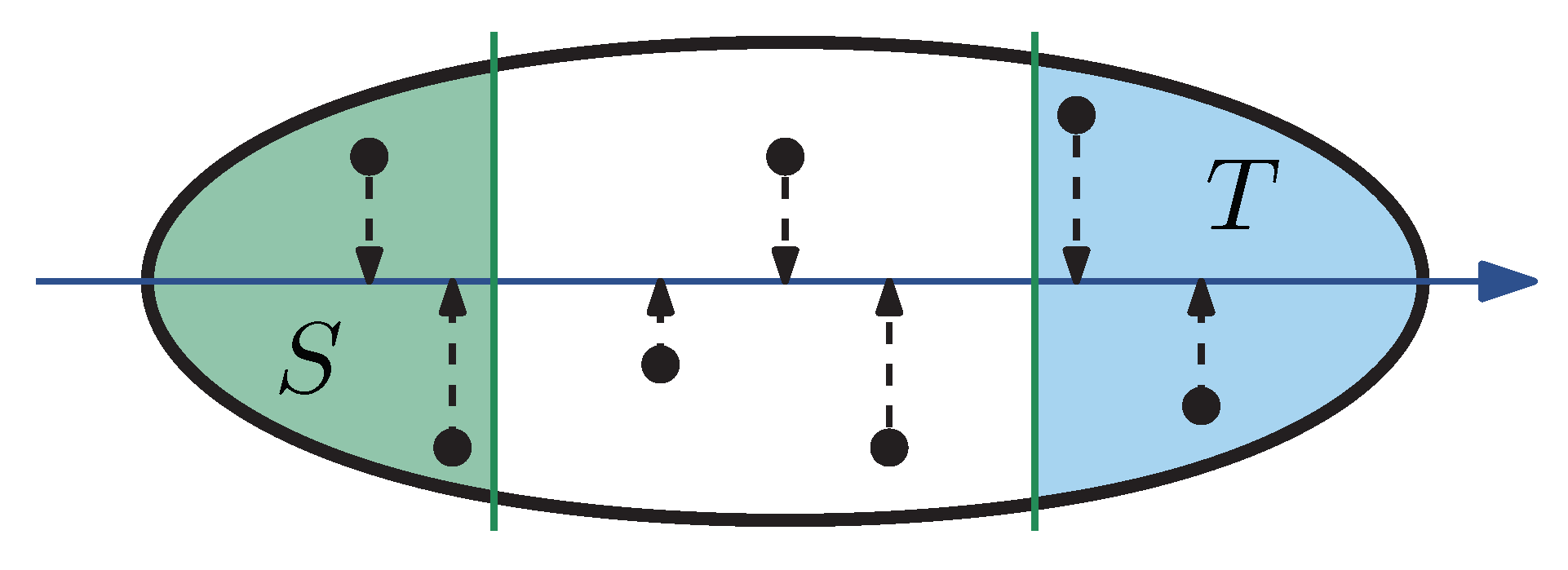
2.3. Inertial Flow
Given a line
, Inertial Flow projects the geographic coordinates of the nodes onto their closest points on
l. The nodes are sorted by order of appearance on
l. For a parameter
, the first
nodes are chosen as
S. Analogously, the last
nodes are chosen as
T. In the next step, a maximum
S–
T flow is computed from which a minimum
S–
T cut is derived.
Figure 1 illustrates the initialization. Instead of line, we use the term
direction. In [
15],
is set to
and four directions are used: West–East, South–North, Southwest–Northeast, and Southeast–Northwest. This simple approach works surprisingly well for road networks.
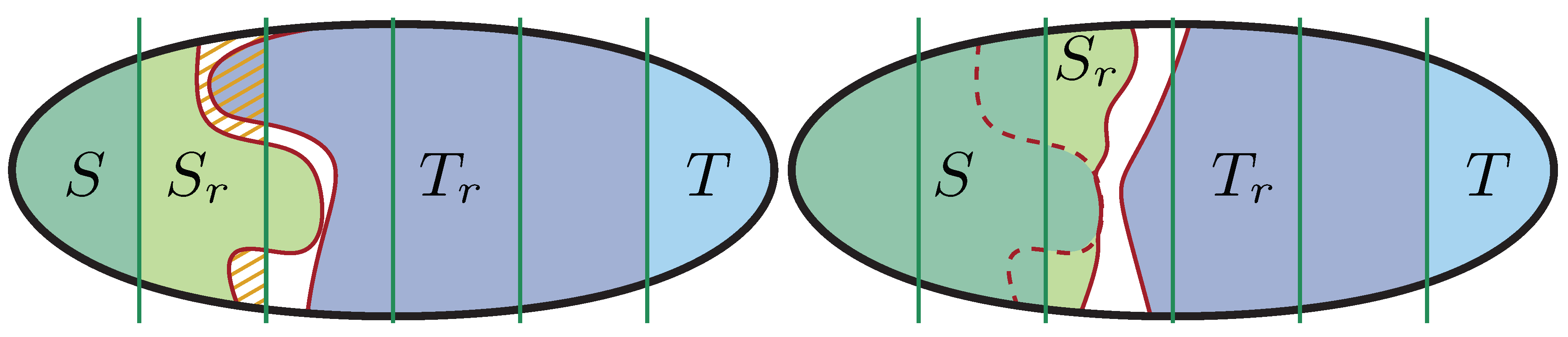
2.4. Combining Inertial Flow and Flowcutter into InertialFlowCutter
One drawback of Inertial Flow is the restriction to an a priori chosen imbalance, i.e., a value of . We enhance FlowCutter by initializing S and T in the same way as Inertial Flow, though with a smaller parameter than proposed for Inertial Flow. Additionally, we pierce cuts with multiple nodes from the Inertial Flow order at once. We call this bulk piercing. This way, we enumerate multiple Inertial Flow cuts simultaneously, without having to restart the flow computations. Furthermore, we can skip some of the first, highly imbalanced cuts of FlowCutter that are irrelevant for our application.
We introduce three additional parameters
and
to formalize bulk piercing. Let
L be a permutation of the nodes, ordered according to a direction. For the source side, we use bulk piercing as long as
S contains at most
nodes. Furthermore, we limit ourselves to piercing the first
nodes of
L. Parameter
influences the step size. The idea is to decrease the step size as the cuts become more balanced. When we decide to apply bulk piercing, we settle the next
nodes to
S, when piercing the source side. To enforce the limit set by
, we pierce fewer nodes if necessary. For the target side, we apply this analogously starting from the end of the order. If bulk piercing can not be applied, we revert to the standard FlowCutter method of selecting single piercing nodes incident to the cut. Additionally, we always prioritize the avoid-augmenting-paths heuristic over bulk piercing. In our experiments, we conduct a parameter study which yields
and
as reasonable choices. In
Figure 2, we show an example for the InertialFlowCutter piercing step.
2.5. Running Multiple InertialFlowCutter Instances
To improve solution quality, we run
instances of InertialFlowCutter with different directions. An instance is called a
cutter. We use the directions
for
and
. To include the directions proposed in [
15],
q should be a multiple of 4. To improve running time, we run cutters simultaneously in an
interleaved fashion as already proposed in [
14]. We always schedule the cutters with the currently smallest flow value to either push one additional unit of flow or derive a cut. For the latter, we improve the balance by piercing the cut as long as this does not create an augmenting path. One standalone cutter runs in
, where
c is the size of the largest output cut. Roughly speaking, this stems from performing one graph traversal, e.g., Pseudo-DFS, per unit of flow. The exact details can be found in [
14]. Flow-based execution interleaving ensures that no cutter performs more flow augmentations than the other cutters. Thus, the running time for
q cutters is
, where
c is the size of the largest found cut among all cutters. We specifically avoid computing some cuts that the standalone cutters would find. Consider the simple example with
, where the second cutter immediately finds a perfectly balanced cut with cut size
c, but the first cutter only finds one cut with cut size
. If the first cutter runs until a cut is found, we invested
work but should only have invested
.
In the case of InertialFlowCutter, it is actually important to employ flow-based interleaving and not just run a cutter until the next cut is found, as after a bulk piercing step, the next cut might be significantly larger. For road networks and FlowCutter, this difference is insignificant in practice, as the cut increases by just one most of the time.
2.6. Customizable Contraction Hierarchies
A Customizable Contraction Hierarchy (CCH) is an index data structure which allows fast shortest path queries and fast adaptation to new metrics (arc weights) in road networks. It consists of three phases: a preprocessing phase which only uses the network topology but not the arcs weights, a faster customization phase which adapts the index to new arc weights, and a query phase which quickly answers shortest path queries.
The preprocessing phase computes a contraction order of the nodes, e.g., via nested dissection, and then simulates contracting all nodes in that order, inserting shortcut arcs between all neighbors of a contracted node. Shortcuts represent two-arc paths via the contracted node.
The customization phase assigns correct weights to shortcuts by processing all arcs in the order ascending by rank of u, i.e., the position of u in the order. To process an arc , it enumerates all triangles where w has lower rank than u and v, and updates the weight of if the path is shorter.
There are two different algorithms for
s–
t queries. For every shortest
s–
t path in the original graph, there is a shortest
s–
t path in the CCH that consists of two paths
and
such that the arcs in the first path are from lower-ranked to higher-ranked nodes, whereas the arcs in the second path are from higher-ranked to lower-ranked nodes [
10]. The first, basic query algorithm performs bidirectional Dijkstra search from
s and
t and relaxes only arcs to higher-ranked nodes. The second query algorithm uses the
elimination tree of a CCH to avoid priority queues, which are typically a bottleneck. In the elimination tree, the parent of a node is its lowest-ranked upward neighbor. The ancestors of a node
v are exactly the nodes in the upward search space of
v in the basic query [
21]. For the
s–
t query, the outgoing arcs of all nodes on the path from
s to the root and all incoming arcs of all nodes on the path from
t to the root are relaxed. The node
z minimizing the distance from
s to
z plus the distance from
z to
t determines the distance between
s and
t.
The query complexity is linear in the number of arcs incident to nodes on the paths from s and t to the root. Similarly, the customization running time depends on the number of triangles in the CCH. Fewer shortcuts result in less memory consumption and faster queries. We aim to minimize these metrics by computing high quality contraction orders.
2.7. Nested Dissection Orders for Road Networks
The framework to compute contraction orders is the same as for FlowCutter in [
14] and our implementation builds upon theirs [
22]. We only exchange the partitioning algorithm and parallelize it. For self-containedness, we repeat it here.
2.7.1. Recursive Bisection
We compute contraction orders via recursive bisection, using node separators instead of edge cuts. This method is also called nested dissection [
13]. Let
be a node separator partition. Then, we recursively compute orders for
and
and return the order of
followed by the order of
followed by
Q.
Q can be in an arbitrary order. We opt for the input order. Recursion stops once the graphs are trees or cliques. For cliques, any order is optimal. For trees, we use an algorithm to compute an order with minimal elimination tree depth in linear time [
23,
24].
In the nested dissection implementation from [
22], a recursive call first computes a node separator
Q, then deletes the edges
incident to that separator and then reorders the nodes in
preorder. Preorder is the order in which nodes are
first visited in a Depth-First-Search from some starting node—in this implementation, the one with smallest ID. The preorder identifies connected components of the new graph, which are the subgraphs to recurse on, as well as assigns local node and arc identifiers for them. This is also done once at the beginning, without computing a separator, in case the input graph is disconnected.
2.7.2. Separators
InertialFlowCutter computes edge cuts. We use a standard construction [
25] to model node capacities as edge capacities in flow networks. It expands the undirected input graph
into a directed graph
. For every node
, there is an
in-node and an
out-node in
, joined by a directed arc
, called the
bridge arc of
v. Furthermore, for every edge
, there are two directed
external arcs
and
. Since we restrict ourselves to unit capacity flow networks, we can not assign infinite capacity to external arcs, and thus, the cuts contain both bridge arcs and external arcs. Bridge arcs directly correspond to a node in the separator. For the external arcs in the cut, we place the incident node on the larger side of the cut in the separator.
2.7.3. Choosing Cuts from the Pareto Cutset
InertialFlowCutter yields a sequence of nondominated cuts with monotonically increasing cut size and balance, whereas standard partitioners yield a single cut for some prespecified imbalance. We need to choose one cut, to recurse on the sides of the corresponding separator. The expansion of a cut is its cut size divided by the number of nodes on the smaller side. This gives a certain trade-off between cut size and balance. We choose the cut with minimum expansion and , i.e., at least 20% of the nodes on the smaller side. While this approach is certainly not optimal, it works well enough. It is not clear how to choose the optimum cut without considering the whole hierarchy of cuts in deeper levels of recursion.
2.7.4. Special Preprocessing
Road networks contain many nodes of degree 1 or 2. The graph size can be drastically reduced by eliminating them in a preprocessing step that is performed only once. First, we compute the largest biconnected component
B in linear time using [
26] and remove all edges between
B and the rest of the graph
G. The remaining graph usually consists of a large
B and many tiny, often tree-like components. We compute orders for the components separately and concatenate them in an arbitrary order. The order for
B is placed after the orders of the smaller components.
A degree-2-chain is a path where all but and . We divide the nodes into two graphs and with degrees at least 3 and at most 2, by computing all degree-2-chains in linear time and splitting along them. If , we insert an edge between x and z since z is in . We compute contraction orders for the connected components of separately and concatenate them in an arbitrary order. Since these are paths, we can use the algorithm for trees. The order for is placed after the one for . We compute degree-2 chains by iterating over all arcs . If and , then x is the start of a degree-2 chain. We follow this chain recursively: As long as , the only arc of y that is not comes next in the chain. If or , the chain is finished at y. This algorithm runs in linear time as it considers every arc at most twice.
2.8. Parallelization
Recursive bisection is straightforward to parallelize by computing orders on the separated blocks independently, using task-based parallelism. This only employs parallelism after the first separators have been found.
Therefore, we additionally parallelize InertialFlowCutter. The implementation of FlowCutter [
22] contains a simple parallelization. In a round, all cutters with the currently smallest cut are advanced to their next cut in parallel. Before the next round, all threads synchronize. This approach exhibits poor core utilization since only a few cutters may have the smallest cut in a round and threads perform different amounts of work, leading to skewed load distribution.
Instead, we employ a simple wait-free task-based parallelization scheme, which guarantees that the cutters with the t currently smallest flow values are making progress, for t threads executing in parallel. Algorithm 2 illustrates this scheme in pseudocode. For every cutter, we store two atomic flags: a free flag, which indicates that currently no task holds this cutter, and an active flag, which indicates that this cutter can still yield a cut with better expansion than previously found cuts. In the beginning, every cutter is active and free.
Recall that q is the number of cutters. We create q tasks, and the task scheduler launches parallel tasks, potentially adding more when resources from other parts of the recursive bisection become available. A task executes a loop in which it first acquires a cutter with the currently smallest flow out of the free and active cutters, then performs a chunk of work on it and releases the cutter again. A chunk of work consists of deactivating the cutter, if it can not improve expansion and otherwise running one Pseudo-Depth-First-Search, which either pushes one unit of flow or derives a cut. If the cut has at least of the nodes on the smaller side and improves expansion, we acquire a lock and store the cut. A task terminates once it fails to acquire a free and active cutter, as there are now more tasks than active cutters.
If less than q tasks are running simultaneously, the tasks switch between cutters. If all cutters are acquired and the task’s currently acquired cutter remains active, we continue working on it, to avoid the overhead of releasing and immediately re-acquiring the same cutter. Note that, due to the parallelization, cuts are not necessarily enumerated in the order of increasing cut size, and dominated cuts may also be reported.
| Algorithm 2: Parallel InertialFlowCutter |
 |
3. Results
In this section, we discuss our experimental setup and results.
3.1. Experimental Setup
In
Section 3.6, we discuss our parameter study to obtain reasonable parameters for InertialFlowCutter. Our remaining experiments follow the setup in [
14], comparing FlowCutter, KaHiP, Metis, and Inertial Flow to InertialFlowCutter, regarding CCH performance as well as cut sizes for different imbalances on the input graph without biconnectivity and degree-2 chain preprocessing. The latter are referred to as top-level Pareto cut experiments. Our benchmark set consists of the road networks of Colorado, California, and Nevada, the USA and Western Europe, see
Table 1, made available during the DIMACS implementation challenge on shortest paths [
27].
The CCH performance experiments compare the different partitioners based on the time to compute a contraction order, the median running time of nine customization runs, the average time of
random
s–
t queries, as well as the criteria introduced in
Section 2.6. Unless explicitly stated as parallel, all reported running times are sequential on an Intel Xeon E5-1630 v3 Haswell processor clocked at 3.7 GHz with 10 MB L3 cache and 128 GB DDR4 RAM (2133 MHz). We additionally report running times for computing contraction orders in parallel on a shared-memory machine with two 8-core Intel Xeon Gold 6144 Skylake CPUs, clocked at 3.5GHz with 24.75 MB L3 cache and 192 GB DDR4 RAM (2666 MHz). InertialFlowCutter is implemented in C++, and the code is compiled with g++ version 8.2 with optimization level 3. We use Intel’s Threading Building Blocks library for shared-memory parallelism. Our InertialFlowCutter implementation and evaluation scripts are available on GitHub [
28].
3.2. CCH Implementation
We used the CCH implementation in RoutingKit [
29]. There are different CCH customization and query variants. RoutingKit implements basic customization with upper triangles instead of lower triangles, no witness searches, no precomputed triangles, and no instruction-level parallelism. We used the sequential customization. For queries, we used elimination tree search. There has been a recent, very simple improvement [
30], which drastically accelerates elimination tree search for short-range queries. It is not implemented in RoutingKit, but random
s–
t queries tend to be long-range, so the effect would be negligible for our experiments.
3.3. Partitioner Implementations and Nested Dissection Setup
In [
14], the KaHiP versions 0.61 and 1.00 are used. We did not re-run the preprocessing for those old versions of KaHiP but used the orders and order computation running times of [
14]. We did re-run customizations and queries. The order computation running times are comparable as the experiments ran on the same machine. We added the latest KaHiP version 2.11, which is available on GitHub [
31]. For all three versions, the
strong preset of KaHiP was used. We refer to the three KaHiP variants as K0.61, K1.00, and K2.11. For the CCH order experiments, we kept versions K0.61 and K1.00 but omitted them for the top-level cut experiments because K2.11 is better for top-level cuts.
We used Metis 5.1.0, available from the authors’ website [
32], which we denote by M in our tables.
We used InertialFlowCutter with directions and denote the configurations by IFC4, IFC8, IFC12, and IFC16, respectively.
We used our own Inertial Flow implementation with the four directions proposed in [
15]. It is available at our repository [
28]. Instead of Dinic algorithm [
33], we used Ford–Fulkerson, as preliminary experiments indicate it is faster. Furthermore, we filtered source nodes that are only connected to other sources and target nodes that are only connected to other targets. Instead of sorting nodes along a direction, we partitioned the node-array such that the first and last
nodes are the desired terminals, using
std::nth_element. These optimizations reduce the running time from 1017 s [
14] down to 450 s for a CCH order on Europe. Additionally, we used flow-based interleaving on Inertial Flow. This was already included in the Inertial Flow implementation used in [
14]. We denote Inertial Flow by I in our tables.
The original FlowCutter implementation used in [
14] is available on GitHub [
22]. We used a slightly modified version that has been adjusted to use Intel’s Threading Building Blocks instead of OpenMP for optional parallelism. All parallelism is disabled for FlowCutter in our experiments. We used FlowCutter with
random source-target pairs and denote the variants by F3, F20, and F100, respectively.
Implementations of Buffoon [
19] and PUNCH [
18] are not publicly available. Therefore, these are not included in our experiments.
We now discuss the different node ordering setups used in the experiments. Metis offers its own node ordering tool
ndmetis, which we used. For Inertial Flow, K1.00 and K2.11, we used a nested dissection implementation, which computes one edge cut per level and recurses until components are trees or cliques, which are solved directly. Separators are derived by picking the nodes incident to one side of the edge cut. For comparability with [
12,
14], we used an older nested dissection implementation for K0.61, which, on every level, repeatedly computes edge cuts until no smaller cut is found for ten consecutive iterations. For InertialFlowCutter and FlowCutter, we employed the setup that was proposed for FlowCutter in [
14] that has also been described in
Section 2.7. Our nested dissection implementation is based on the implementation in the FlowCutter repository [
22]. We made minor changes and parallelized it, as described in
Section 2.8.
We tried to employ the special preprocessing techniques for KaHiP 2.11. While this made order computation faster, the order quality was much worse regarding all criteria.
Starting with version 1.00, KaHiP includes a more sophisticated multilevel node separator algorithm [
34]. It was omitted from the experiments in [
14] because it took 19 hours to compute an order for the small California graph, using one separator per level, and did not finish in reasonable time on the larger instances. Therefore, we still exclude it.
3.4. Order Experiments
In this section, we compare the different partitioners with respect to the quality of computed CCH orders and running time of the preprocessing.
Table 2 contains a large collection of metrics and measurements for the four road networks of California, Colorado, Europe, and the USA. Recall that the query time is averaged over
queries with distinct start and end nodes chosen uniformly at random, the customization time is the median over nine runs. The order computation time is from a single run, since it is infeasible to run certain partitioners multiple times in a reasonable timeframe.
3.4.1. Quality
Over all nodes
v, we report the average and maximum number of ancestors in the elimination tree, as well as the number of arcs incident to the ancestors. These metrics assess the search space sizes of an elimination tree query. The query times in
Table 2 are correlated with search space size, as expected. The partitioner with the smallest average number of nodes and arcs in the search space always yields the fastest queries. Furthermore, we report the number of arcs in the CCH, i.e., shortcut and original arcs, the number of triangles, and an upper bound on the treewidth, which we obtained using the CCH order as an elimination ordering. A CCH is essentially a chordal supergraph of the input. Thus, CCHs are closely related to tree decompositions and elimination orderings. The relation between tree decompositions and Contraction Hierarchies is further explained in [
35]. A low treewidth usually corresponds to good performance with respect to the other metrics. However, as the treewidth is defined by the largest bag in the tree decomposition which may depend on the size of few separators and disregards the size of all smaller separators, this is not always consistent. In the context of shortest path queries, a better average is preferable to a slightly reduced maximum.
On the California and USA road networks, IFC12 yields the fastest queries and smallest average search space sizes, while on Europe IFC8 does. On Colorado, our smallest road network, F100 is slightly ahead of the InertialFlowCutter variants by to microseconds query time. IFC16 yields the fastest customization times for Colorado, Europe, and the USA, while IFC12 yields the fastest customization times for California. Customization times are correlated with the number of triangles. However, for Europe and the USA, the smallest number does not yield the fastest customizations. Even though we take the median of nine runs, this may still be due to random fluctuations.
FlowCutter with at least 20 cutters has slightly worse average search space sizes and query times than InertialFlowCutter for California and the USA but falls behind for Europe. Thus, InertialFlowCutter computes the best CCH orders, with FlowCutter close behind. The different KaHiP variants and Inertial Flow compute the next best orders, while Metis is ranked last by a large margin.
The ratio between maximum and average search space size is most strongly pronounced for Inertial Flow. This indicates that Inertial Flow works well for most separators, but the quality degrades for a few. InertialFlowCutter resolves this problem.
There is an interesting difference in the number of cutters necessary for good CCH orders with InertialFlowCutter and FlowCutter. In [
14], F20 is the recommended configuration. The performance differences between F20 and F100 are marginal (except for Europe). However, using just three cutters seems insufficient to get rid of bad random choices.
For the InertialFlowCutter variants, four cutters suffice most of the time. The search space sizes, query times and customization times are very similar. This is also confirmed by the top-level cut experiments in
Section 3.5. It seems the Inertial Flow guidance is sufficiently strong to eliminate bad random choices. Again, only for Europe, the queries for IFC4 are slower, which is why we recommend using IFC8. The better query running times justify the twice as long preprocessing.
Europe also stands out when comparing Inertial Flow query performances. For Europe, Inertial Flow only beats Metis, but, for the USA, it beats all KaHiP versions and Metis. The query performance difference of 57 microseconds between Inertial Flow and IFC4 for Europe suggests that the incremental cut computations of InertialFlowCutter make a significant difference and are worth the longer preprocessing times compared to Inertial Flow.
3.4.2. Preprocessing Time
Previously, CCH performance came at the cost of high preprocessing time. We compute better CCH orders than FlowCutter in a much shorter time.
KaHiP 0.61 and KaHiP 1.00 are by far the slowest. KaHiP 2.11 is faster than F100 but slower than F20. All InertialFlowCutter variants are faster than F20. IFC8 and F3 have similar running times. Metis is the fastest by a large margin, and Inertial Flow is the second fastest.
The two old KaHiP versions are slow for different reasons. As already mentioned, K0.61 computes at least 10 cuts, as opposed to K1.00 and K2.11. K1.00 is slow because the running time for top-level cuts with
increases unexpectedly, according to [
14].
Using 16 cores and IFC8, we compute a CCH order of Europe in just 242 s, with 2258 s sequential running time on the Skylake machine. This corresponds to a speedup of 9.3 over the sequential version. See
Table 3. Note that, due to using eight cutters, at most eight threads work on a single separator. Therefore, in particular for the top-level separator, at most 8 of the 16 cores are used. The top-level separator alone needs about 50 s using eight cores. Due to unfortunate scheduling and unbalanced separators, it happens also at later stages that a single separator needs to be computed before any further tasks can be created. Using eight cores, we get a much better speedup of 6.8 for Europe; up to four cores, we see an almost perfect speedup for all but the smallest road network. This is because some cutters need less running time than others. Thus, there is actually less potential for parallelism than the number of cutters suggests.
3.5. Pareto Cut Experiments
For the top-level cut experiments, we permute the nodes in preorder from a randomly selected start node, using the same start node for all partitioners. As discussed in
Section 2.7, this is part of the recursive calls in the nested dissection implementation from [
22]. We include it here to recreate the environment of a nested dissection on the top level.
In
Table 4,
Table 5,
Table 6 and
Table 7, we report the found cuts for various values of
for all road networks. We use the partitioners KaHiP 2.11, IFC4, IFC8, IFC12, F3, F20, Metis, and Inertial Flow. We also report the actually achieved imbalance, the running time, and whether the sides of the cut are connected (•) or not (∘). We report
only if perfect balance was achieved; otherwise, if the rounded value is
, we report
. KaHIP was not able to achieve perfect balance for any of the graphs if perfect balance was desired. We note this by crossing out the respective values. This is due to our use of the KaHiP library interface that does not support enforcing balance. Metis simply rejects
, which is why we mark the corresponding entries with a dash. Perfect balance is not actually useful for the application. We solely include it to analyze the different Pareto cuts.
Note that for FlowCutter and InertialFlowCutter, the running time always includes the computation of all more imbalanced cuts, i.e., to generate the full set of cuts, only the running time of the perfectly balanced cut is needed, while for all other partitioners, the sum of all reported running times is needed.
Concerning the performance, Metis wins, but almost all reported cuts are larger than the cuts reported by FlowCutter, InertialFlowCutter, and KaHiP. Inertial Flow is also quite fast but, due to its design, produces cuts that are much more balanced than desired and thus can not achieve as small cuts as the other partitioners.
KaHIP achieves exceptionally small, highly balanced cuts on the Europe road network. On the other road networks, it is similar to or worse than F20 in terms of cut size. This is due to the special geography of the Europe road network. It excludes large parts of Eastern Europe, which is why there is a cut of size 2 and
imbalance that separates Norway, Sweden, and Finland from the rest of Europe. For
, KaHiP computes a cut with 112 edges, which separates the European mainland from the Iberian peninsula, Britain, Scandinavia minus Denmark, Italy, and Austria [
14]. The Alps separate Italy from the rest of Europe. Britain is only connected via ferries, and the Iberian peninsula is separated from the remaining mainland by the Pyrenees. One side of the cut is not connected because the only ferry between Britain and Scandinavia runs between Britain and Denmark. FlowCutter is unable to find cuts with disconnected sides without a modified initialization. By handpicking terminals for FlowCutter, a similar cut with only 87 edges and
imbalance, which places Austria with the mainland instead, is found in [
14]. However, it turns out that the FlowCutter CCH order using the 87 edge cut as a top-level separator is not much better than plain FlowCutter. This indicates that it does not matter at what level of recursion the different cuts are found.
For large imbalances, KaHIP seems unable to leverage the additional freedom to achieve the much smaller but more unbalanced cuts, like the ones reported by InertialFlowCutter and FlowCutter. This has already been observed for previous versions of KaHIP [
14]. In terms of running time, KaHIP and F20 are the slowest algorithms. InertialFlowCutter is in all three configurations an order of magnitude faster than F20. Up to a maximum
of
, the three variants report almost the same cuts. Apart from the very imbalanced
cuts, the cuts are also at most one edge worse than F20. Only for more balanced cuts more cutters give a significant improvement. Here, in particular on the Europe road network, F20 is also significantly better than InertialFlowCutter. In the range between
and
, which is most relevant for our application, there is thus no significant difference between F20 and InertialFlowCutter, regardless of the number of cutters. This indicates that on the top level, the first four directions seem to cover most cuts already. On the other hand, for highly balanced cuts, the geographic initialization does not help much, as can be seen from the much worse cuts for InertialFlowCutter. Here, just having more cutters seems to help.
3.6. Parameter Configuration
In this section, we tune the parameters
of InertialFlowCutter. Our goal is to achieve much faster order computation without sacrificing CCH performance. Recall that
is the fraction of nodes initially fixed on each side,
is—roughly speaking—a stepsize,
is the threshold up to how many nodes on a side of the projection we perform bulk piercing, and similarly,
for how many settled nodes on a side.
Table 8 shows a large variety of tested parameter combinations for InertialFlowCutter with eight directions on the road network of Europe. We selected the parameter set
based on query and order computation time. The best entries per column are highlighted in bold. Furthermore, color shades are scaled between values in the columns. Darker shades correspond to lower values, which are better for every measure.
First, we consider the top part of
Table 8, where we fix
to
and try different combinations of
. While the number of triangles and customization times are correlated, the top configurations for these measures are not the same interestingly. The variations in search space sizes, customization time (27 ms), and query time (3
s) are marginal. At the bottom part of
Table 8, we try different values of
with the best choices for the other parameters. As expected, larger values for
accelerate order computation and slightly slow down queries. In summary, InertialFlowCutter is relatively robust to parameter choices other than for
, which means users do not need to invest much effort on parameter tuning.


