Correspondence between Multilevel Graph Partitions and Tree Decompositions

Abstract

We present a mapping between rooted tree decompositions and node separator based multilevel graph partitions. Significant research into both tree decompositions and graph partitions exists. We hope that our result allows for an easier knowledge transfer between the two research avenues.

1. Introduction

Graph partitioning aims to divide a graph into two or more roughly equally sized parts by removing a small number of nodes or edges. By recursively partitioning these parts, a tree-like hierarchy of partitions is created. Graph partitioning is a well-known, well-researched, active research field with many applications [1,2]. Graph partitioning papers usually contain experiments and are often written by the applied experimental algorithms community. Experiments on large-scale graphs with millions of nodes are very common [3,4,5,6,7,8].

Tree decompositions aim to decompose a graph into a tree-like structure. The width then basically denotes how similar a tree decomposition is to a tree. For some hard problems, there are algorithms that are efficient on graphs with tree decompositions of small width. Tree decomposition theory is also a well-known, active research field with a lot of activity. For an overview, we refer to the works of Blair and Peyton [9], Bodlaender [10] and Bodlaender [11]. While experimental tree decomposition studies exist, purely theoretical tree decomposition papers are common. Progress in this field is mostly driven by the theoretical algorithms community. Experiments on large-scale graphs with millions of nodes are unfortunately rare.

In this paper, we present a theorem that states that graph partitions and tree decompositions are two different views onto essentially the same mathematical object. Our result brings both research fields closer together.

We are not the first to discover a connection between graph partitioning and tree decomposition. For example, METIS [12] is well-known in the graph partitioning community and can be used to compute node elimination orders, a concept closely tied to tree decompositions. Elimination orders are used to efficiently solve sparse systems of linear equations, which has a myriad of real-world applications. However, to the best of our knowledge, nobody has presented a precise one-to-one mapping between multilevel graph partitions and tree decompositions. This mapping is the contribution of our paper.

Besides formally proving the correspondence, we additionally aim to make our exposition accessible to readers familiar with only one of the two research fields. We illustrate all definitions and theorems using running examples. Additionally, we present tree decompositions of large road graphs computed using the algorithms of Hamann and Strasser [13] and Dibbelt et al. [14]. Hopefully, these examples allow readers to get an intuition for the structure of tree decompositions in large-scale real world graphs.

In Section 2, we present the tree decomposition definition. In Section 3, we formalize the graph partitioning paradigm. In Section 4, we present our main result, a one-to-one mapping between rooted tree decompositions and node-based multilevel partitions. Finally, in Section 5, we illustrate tree decompositions in road graphs.

2. Tree Decomposition

We denote by $G=(V,E)$ an undirected graph. G has neither multiedges nor loops. Throughout this paper, we require that G is not empty. All tree decompositions and multilevel partitions are computed with respect to the same given graph G. G is never modified in this paper. All stated modifications and constructions refer to a multilevel partition or a tree decomposition of G.

A tree decomposition is a tree T with node multiset $\mathcal{X}$. The tree T is called backbone and its nodes are called bags. A bag is set of nodes of graph G. Every tree decomposition must fulfill the following requirements:

1.

For every node $u\in V$, there is a bag $X\in \mathcal{X}$ such that $u\in \mathcal{X}$.

2.

For every edge $\{u,v\}\in E$, there is a bag $X\in \mathcal{X}$ such that $u\in X$ and $v\in X$.

3.

For every pair of bags $X\in \mathcal{X}$ and $Y\in \mathcal{X}$, every bag Z along the unique path in T from X to Y must contain the intersection of X and Y, i.e., $X\cap Y\subseteq Z$.

In this paper, we refer to them as node, edge, and path requirements. Without loss of generality, we assume throughout this paper that there are at least two bags.

The width $w\left(T\right)$ of a tree decomposition T is the maximum bag size minus one, i.e., $w\left(T\right)={max}_{x\in X}\left|x\right|-1$. In most settings, tree decompositions of small width are desired. The minimum width of any tree decomposition is the tree width of a graph G.

A rooted tree decomposition additionally has a root bag $X_r$. With respect to a root bag, every bag X except the root itself has a parent bag $X_p$. A bag is a child of its parent bag. Similarly, a bag Y is a descendant of X, if X is on the path from Y to the root. X is a descendant of X. We denote by ${\mathcal{X}}_d$ a set of descendant bags. A bag without children is a leaf bag. As we assumed that there are at least two bags, the root bag is never a leaf bag.

To establish a one-to-one correspondence with multilevel partitions, we require two additional technical requirements:

4.

no leaf bag is a subset of its parent bag; and

5.

for every non-root bag X and node $x\in X$, such that the parent bag but no child bag of X contains x, removing x from X must result in a violation of the edge property.

In this paper, we refer to the fourth property as leaf property and the fifth property as small bag property.

Luckily, a rooted tree decomposition that does not fulfill the leaf property can easily be transformed into one that does by removing the offending leaf bags. Similarly, by removing offending nodes, a tree decomposition can be constructed that fulfills the small bag property. Important metrics such as the width of a tree decomposition cannot be increased by these transformations. Both properties thus only codify that a certain class of superfluous bags and nodes must not exist.

In Figure 1, we present an example tree decomposition that we use as running example throughout this paper. The first tree decomposition property requires that for every edge in G there is a bag x in T that contains both endpoints. For example, the endpoints of the edge $\{g,p\}$ are contained in the bag $\{f,g,p,c\}$. The property does not require that the bag is unique. For example, the endpoints of the edge $\{m,o\}$ are contained in two bags, namely $\{o,m,p\}$ and $\{n,o,m\}$. The third tree decomposition property requires that every node in the intersection of two bags is in every bag between them. For example, p is part of the bags $\{f,m,p\}$ and $\{p,r,i\}$. The property requires that p is also part of the bags on the path between. These are $\{f,p,c\}$, $\{p,c\}$, and $\{p,c,i\}$.

3. Graph Partitioning

The graph partitioning paradigm consists of dividing a graph into two or more smaller parts that are loosely connected. This is a very useful tool to extend divide-and-conquer algorithms to graphs. A complex problem, such as graph coloring [15], can be solved by reasoning in isolation about each part. From the parts’ solutions, a global solution for the whole graph can be constructed. This approach can be applied recursively over many levels. In this case, a multilevel partition is used.

In the literature, many different graph partitioning variants exist [1]. Many papers divide the graph along edge cuts. This means that the input graph is disconnected by removing edges. We say that this form of graph partitioning is edge-based. A slightly less frequently used graph partitioning variant uses node separator, i.e., the input graph is disconnected by removing nodes. We say that this graph partitioning variant is node-based.

In this section, we present a formalization of both edge-based and node-based graph partitions and highlight the differences. Our theorem, in the next section, establishes a connection between node-based multilevel graph partitions and tree decompositions.

3.1. Edge-Based Graph Partition

An edge-based graph partition of a graph $G=(V,E)$ is a set $\mathcal{C}$ of subsets of V. The node sets of $\mathcal{C}$ must form a disjoint partition of V. $\mathcal{C}$’s elements are called cells or partitions. In the rest of this paper, we use the term cells. Edges with endpoints in more than one cell are cut edges. The number of cut edges is the cut size.

Think of edge-based graph partitioning as cutting with scissors through some edges of G. The cut edges are the edges that the scissors pass through. $\mathcal{C}$ is the set of parts into which G is decomposed.

3.2. Node-Based Graph Partition

A node-based graph partition of a graph $G=(V,E)$ is a set $\mathcal{C}$ of subsets of V. No node of V may be contained in more than one set in $\mathcal{C}$. Further, we require that there is no edge $\{u,v\}\in E$ such that u and v are in different cells of $\mathcal{C}$. The set of nodes of V that are in no set of $\mathcal{C}$ is called separator. A common objective is to minimize the separator size.

Node-based partitioning is very similar to edge-based partitioning. Think of it as cutting through nodes instead of cutting through edges. Figure 2 illustrates edge- and node-based partitions.

A node-based partition can be derived from an edge-based partition. For every cut edge, an endpoint is selected and inserted into the constructed separator.

3.3. Touching Cells

Graph partitions can be described using a touch relation between cells. In the edge-based setting, two cells $C_1$ and $C_2$ touch, if their intersection is non-empty, i.e., $C_1\cap C_2\ne \varnothing$. In the node-based setting, they also touch if there exists an edge $\{u,v\}\in E$ such that one endpoint is in $C_1$ and the other in $C_2$. Figure 3 illustrates the touch definition. Node- and edge-based partitioning can be viewed as covering a graph using non-touching cells. We consider a graph to be covered, if no further non-touching cell can be added, which, in the node-based setting, does not necessarily mean that every node is covered.

3.4. Multilevel Graph Partition

A multilevel graph partition is obtained by recursively partitioning a graph $G=(V,E)$. The cells obtained in the first step are partitioned again. This process is repeated over several levels. The union of all cells obtained in every recursion step is called the set $\mathcal{C}$ of cells. By definition, V is also cell. The set of cells $\mathcal{C}$ is the multilevel graph partition. This recursive definition models closely how partition-based divide-and-conquer graph algorithms operate. However, to prove properties about multilevel partitions, we use a different, equivalent, non-recursive definition described in the next paragraph. We use this different definition in the remainder of this paper.

A multilevel graph partition is a rooted tree P with node multiset $\mathcal{C}$ of cells and root V. Cells are subsets of V. We require that, for every multilevel graph partition $\mathcal{C}$:

• V is a cell, i.e., $V\in \mathcal{C}$;
• no cell is empty;
• all touching cells are totally ordered by set inclusion, i.e., $\forall C_1,C_2\in \mathcal{C}:C_1\mathrm{touches}{C}_2\Rightarrow C_1\subseteq C_2\vee C_2\subseteq C_1$; and
• for all cells $C_1,C_2\in \mathcal{C}$: if $C_1⊊C_2$, $C_2$ is an ancestor of $C_1$, if $C_1=C_2$, $C_1$ is an ancestor of $C_2$ or $C_2$ is an ancestor of $C_1$.

Analogous to the tree decomposition assumption, we assume without loss of generality throughout this paper that there are at least two cells.

We define the children of a cell C as the cells such that C is the parent. We call a cell D descendant of C, C is on the path from D to the root. In particular, C is a descendant of C. A cell that has no child is a leaf cell.

Finally, we introduce three terms that are only well-defined in the node-based setting. The boundary $B_C$ of a cell C is the set of nodes adjacent to C in G, i.e., $u\in B_C$ if there exists an edge $\{u,v\}$ with $u\notin C$ and $v\in C$. The separator $S_C$ of a cell C is C minus all of C’s children. If C has no children, then C’s separator is equal to C, i.e., $S_C=C$.

Figure 4 depicts an example node-based multilevel partition of the running example. The green cell is the V cell. Its separator $S_V$ is $\{p,c\}$ and its boundary is empty. The children of V are the orange cells. Another example is the blue cell $C_1=\{q,r,j,k,l\}$ in the bottom right. Its separator $S_{C_1}$ is $\left\{r\right\}$ and its boundary $B_{C_1}$ is $\{i,p\}$. It has two children, namely $C_2=\left\{q\right\}$ and $C_3=\{j,k,l\}$. The cell $C_2$ has no children. Its separator $S_{C_2}$ is therefore equal to $\left\{r\right\}$, i.e., $C_2$. The boundary of $C_2$ is $\{p,i,r\}$. Finally, the cell $C_3$ has only one child, namely $\{k,l\}$. The boundary $B_{C_3}$ is $\{i,r\}$ and the separator $S_{C_3}$ is $\left\{j\right\}$.

4. Correspondence between Multilevel Graph Partitioning and Tree Decompositions

In this section, we present the central result of our paper: a theorem to translate tree decomposition and multilevel graph partitions. Formally, it states:

Theorem 1.

There exists a one-to-one mapping between rooted tree decompositions that fulfill leaf and small bag properties and multilevel node-based graph partitions.

Our proof is structured as follows: We first describe algorithms to perform the mapping in both directions. Next, we prove that these two algorithms are correct, i.e., that the constructed tree decomposition and multilevel partition fulfill the required properties. Finally, we show that chaining both algorithms is the identity.

4.1. Multilevel Partition to Tree Decomposition

In this subsection, we describe an algorithm named MLP2TD to convert a multilevel partition P into a rooted tree decomposition T. For every cell C of P, the algorithm creates a bag $X_C$ with the nodes on the boundary and the separator of C, i.e.,

$$X_C=B_C\cup S_C$$

For every non-root cell C of P with parent $C_P$, the algorithm creates a backbone edge from $X_C$ to $X_{C_P}$. The algorithm sets the root bag to the bag $X_V$ corresponding to the root cell of P.

4.2. Tree Decomposition to Multilevel Partition

In this subsection, we describe an algorithm named TD2MLP that converts a rooted tree decomposition with leaf property T into a multilevel partition P. For every bag X, the algorithm computes a cell $C_X$. The cell $C_{X_r}$ of the root bag $X_r$ is by definition V. TD2MLP computes all other cells using the formula

$$C_X=\left(\bigcup {\mathcal{X}}_d\right)\setminus \left(X\cap X_p\right)$$

where ${\mathcal{X}}_d$ is the set of descendant bags of X, which includes X, and $X_p$ is the parent bag of X. For every non-root bag X of T with parent $X_p$, the algorithm creates a tree edge from $C_X$ to $C_{X_P}$.

The constructed multilevel partition has useful properties. Lemma 11 shows that $X\setminus X_p$ corresponds to the separator of $C_X$, i.e.,

$$S_{C_X}=X\setminus X_p$$

Similarly, Lemma 10 shows that, if the tree decomposition additionally fulfills the small bag property, $X\cap X_p$ corresponds to the boundary of $C_X$, i.e.,

$$B_{C_X}=X\cap X_p$$

4.3. Asymptotic Running Times

The running times of MLP2TD and TD2MLP depend on detailed in-memory representations used for multilevel partitions and tree decompositions. We represent node-based multilevel partition cells in-memory by their separator. Additionally, we store the parent/child relationships among cells. This has the nice property that the amount of storage needed to represent any multilevel partition P is linear in the number of nodes of the graph and the tree. Each cell is the union of its children and its separator. Therefore, the nodes of each cell C can be recovered by a bottom-up traversal that builds the union of the separator of C and all children of C.

Our analysis assumes an implementation that stores a bag X as an array of node IDs. The tree backbone stores for every bag the parent bag’s ID and an array of child bag IDs. Cells are represented as array containing the separator $S_C$. Further, we store the parent and the children cell’s IDs. In Algorithms 1 and 2, we present two recursive functions that implement MLP2TD and TD2MLP, respectively. We do not explicitly build a tree-backbone or the multilevel partition tree in these functions but just output bags or separators. As both trees are traversed recursively, it is however easy to build them.

Algorithm 1: Recursive function that implements MLP2TD.

Algorithm 2: Recursive function that implements TD2MLP.

For MLP2TD, we need to calculate the boundary of each cell. OutputBags() in Algorithm 1 recursively calculates the boundary of each cell represented by a separator S. It first calls itself on all children and accumulates their boundaries in B. Then, it marks all nodes in the separator and adds their neighbors to B. Note that marks are global and never cleared. The boundary is then obtained by removing all marked nodes from B. By building the union of S and B, it then outputs the corresponding bag X. To show its correctness, we need to show that OutputBags indeed returns the boundary of the cell represented by S.

Lemma 1.

In Algorithm 1,OutputBagsreturns the boundary of the cell represented by S.

Proof. 

The proof consists of three steps: First, we show that we obtain a suitable set of candidates on lines 4–9. Then, we show that line 10 removes all nodes that are not in the boundary. As a last step, we show that line 10 does not remove any nodes that are in the boundary.

As a cell C is the union of the children of C and C’s separator, any node in the boundary of C must either be in the boundary of one of C’s children or a neighbor of a node of C’s separator. Therefore, after lines 4–9, B is a superset of the boundary. Further, any node that is in B but not in the boundary is part of C.

Due to the recursive calls of OutputBags, all separators of children of S are marked and thus at least all nodes in C are marked. Therefore, in line 10, all nodes of C are removed.

What remains to be shown is that we have not marked too many nodes. Note that marks are never cleared. We only mark nodes that are contained in a cell that is processed. Thus, any node may be marked unless it is only contained in ancestors of C. Any cell $C_b$ that contains one of C’s boundary nodes touches C and is thus, according to the definition of multilevel partitions, either a descendant or an ancestor of C. As $C_b$ contains a node that is not in C, it must be an ancestor of C. Therefore, $C_b$ is processed after C. This means that no node of the boundary has been marked. □

Lemma 2.

The running time of Algorithm 1 is linear in the size of the graph and the tree decomposition it computes.

Proof. 

As every node is part of exactly one separator, line 9 is executed exactly once for every node and its total running time is thus linear in the graph. The trickiest step is to implement B in time linear in the final size. For this, we use a combination of an array of size $\left|V\right|$ to mark its members and another array that contains the actual elements. We reset the marks at the end of every function call. This allows adding elements without adding duplicates in constant time and then allows to list all elements in time linear in the number of elements. In line 6, we cannot merge the boundary yet but instead first need to store all boundaries as we need the data structure still for the recursive calls. Instead, we merge the boundaries after the loop of recursive calls. Note that we merge every boundary at most once, therefore, the running time is linear in the size of all boundaries combined and thus linear in the output size. □

Algorithm 2 provides a recursive function that implements TD2MLP. Its function OutputSeparators() is called for each bag X recursively, starting with the root bag. OutputSeparators() starts by outputting the nodes in the bag X except nodes that are marked. Then, it marks all nodes in X and calls itself recursively. Algorithm 2 runs in time linear in the input, as it processes the elements of every bag X only a constant number of times. What remains to be shown is that line 4 indeed outputs the separator as defined in TD2MLP.

Lemma 3.

Line 4 calculates $X\setminus X_p$ and thus S as defined inTD2MLP.

Proof. 

We need to show that all nodes in $X_p$ are marked and that no nodes in $X\setminus X_p$ are marked, i.e., that we do not omit any nodes. As all nodes in X are marked in line 5 before the recursive call in line 7, all nodes in $X_p$ are marked when X is processed. However, additional nodes may be marked. We must exclude that there is a node $u\in X$ such that $u\notin X_p$ but u is marked, i.e., there is a bag Y such that $u\in Y$ and Y has been processed already. Assume such a node u existed. As the recursion happens after the output, no descendants of X have been processed yet. Therefore, in the backbone tree, the path from X to Y is via $X_p$. Due to the path requirement, this means that $u\in X_p$, but we chose u such that $u\notin X_p$. Therefore, such a node u does not exist and therefore we do not remove too many nodes from X and thus line 4 outputs exactly the separator $S_X$. □

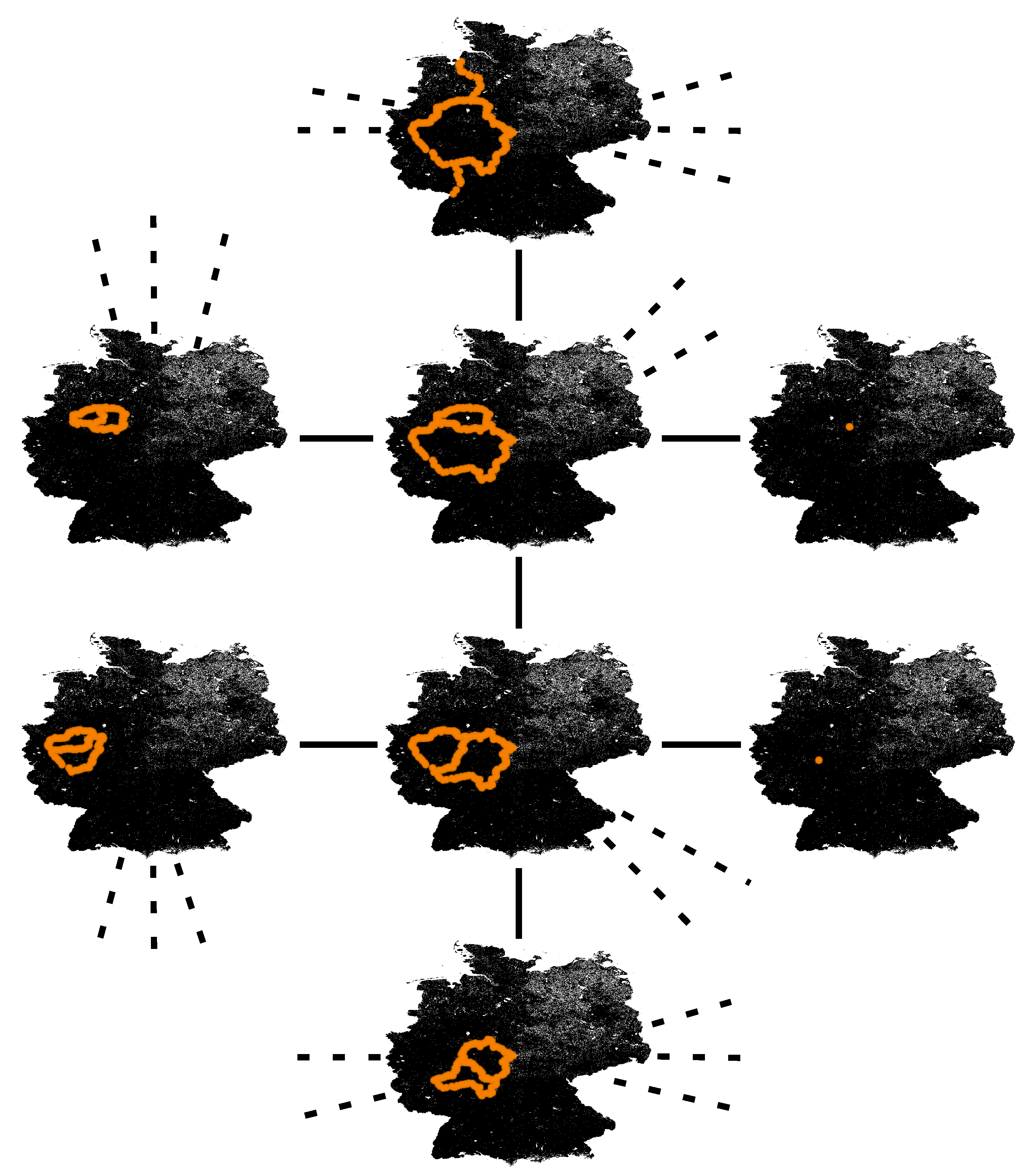
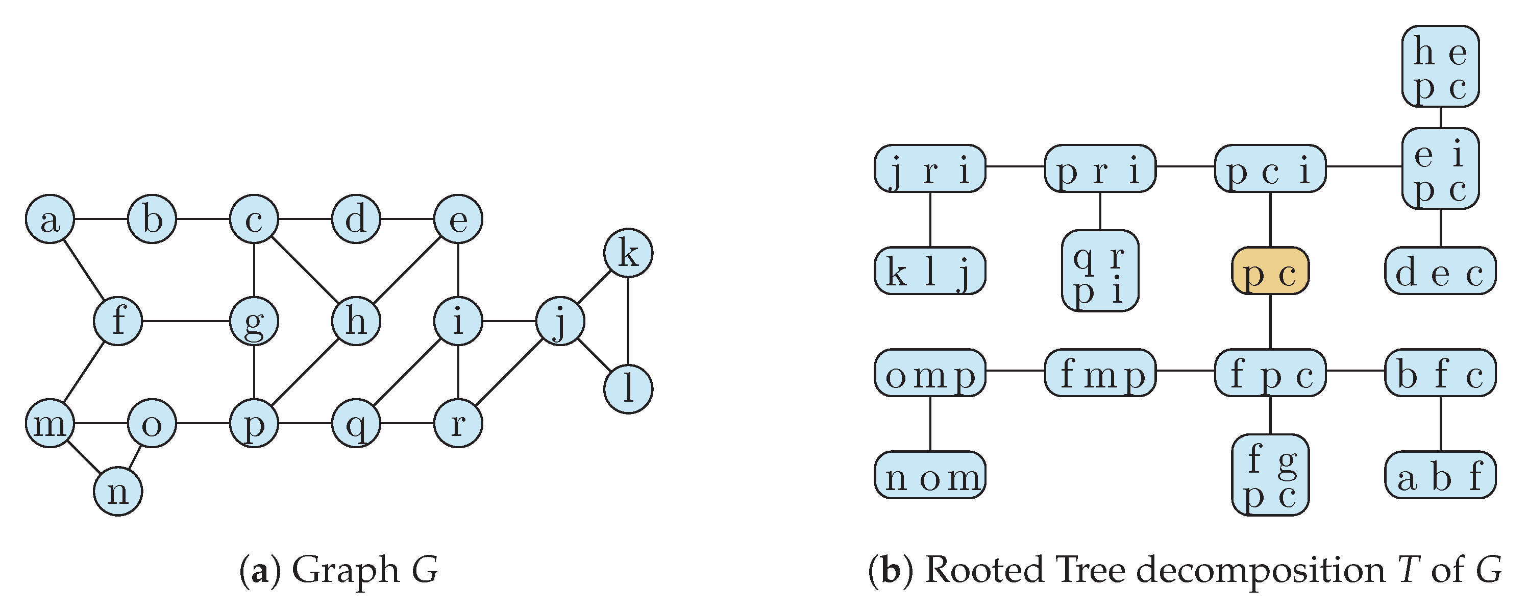
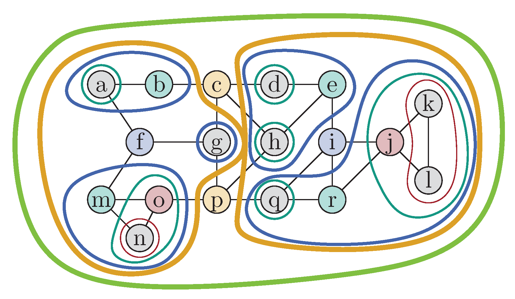
4.4. Example Transformation

The multilevel node-based partition of Figure 4 corresponds to the rooted tree decomposition of Figure 1b. Consider the left blue cell $C=\{m,o,p\}$, boundary $B_C=\{f,p\}$ and separator $S_C=\left\{m\right\}$. The corresponding bag X is $C\setminus S_C=\{f,m,p\}$, which is a bag in Figure 1b.

Alternatively, consider the bag $X=\{e,p,i,c\}$ and denote by C the corresponding cell. The parent $X_p$ is the bag $\{p,i,c\}$. The descendants are ${\mathcal{X}}_d=\left\{\{h,e,p,c\},\{d,e,c\}\right\}$. Using the formulas, we obtain $B_C=\{p,i,c\}$. The separator $S_C$ is $\left\{e\right\}$. We therefore have $\bigcup {\mathcal{X}}_d=\{e,p,i,c,h,d\}$ and thus the cell is $C=\{e,h,d\}$.

Finally, let us consider a different example graph. It have three nodes a, b, and c. There are no edges, i.e., the graph is not connected. Further consider a multilevel partition with five cells, namely $\{a,b,c\}$, $\{a,b\}$, $\left\{a\right\}$, $\left\{b\right\}$, and $\left\{c\right\}$. This translates into a tree decomposition, with two empty bags. $\{a,b,c\}$ corresponds to ∅, and $\{a,b\}$ corresponds to ∅, and the cells $\left\{a\right\}$, $\left\{b\right\}$, and $\left\{c\right\}$ are equal to their bag. Fortunately, our algorithms also work on this multilevel partition. The two ∅ bags are discerned by their position in the backbone. The children bags of the bag corresponding to the cell $\{a,b\}$ are $\left\{a\right\}$ and $\left\{b\right\}$. The union over all descendants is $\varnothing \cup \left\{a\right\}\cup \left\{b\right\}$, which is equal to the original cell $\{a,b\}$. The construction for $\{a,b,c\}$ is analogous. This example shows, that in corner cases, it is important that the sets of bags and cells are multisets.

4.5. Correctness Proof

It remains to formally prove our theorem. In Theorems 2 and 3 in this section, we first show that the two algorithms are correct. In Section 4.6, we then show that they form a bijection.

Theorem 2.

Given a multilevel partition,MLP2TDconstructs a rooted tree decomposition with leaf and small bag properties.

Proof. 

We need to show that the three requirements laid out in the tree decomposition definition are fulfilled by the constructed tree decomposition. Further, we need to show that the leaf and the small bag properties hold.

We first show that the node requirement is fulfilled, i.e., that every node is in a bag. A node v in a cell C is either in C’s separator $S_C$ or in a child of C. By applying this observation iteratively and using that the number of cells is finite, we conclude that every node that is in some cell is in some separator. As every cell’s separator is part of its constructed bag, every node in a cell is in a bag. Further, as every node is in the root cell V, we conclude that every node is in some separator and thus in some bag.

Next, we prove that the edge requirement is fulfilled. We need to show that for every edge $\{u,v\}$ there exists a bag X such that u and v are part of X. As touching cells are ordered by inclusion, there is a cell $C_u$ that contains u such that no child of $C_u$ contains u. u is in the separator of $C_u$ and thus in the bag corresponding to $C_u$. Let $C_v$ be analogously a cell that contains v such that no child of $C_v$ contains v. If $C_u=C_v$, then the bag corresponding to $C_u$ is the required X. Otherwise, we observe that the existence of $\{u,v\}$ implies that $C_u$ and $C_v$ touch each other. The multilevel partition definition thus requires that $C_u$ and $C_v$ are ordered by inclusion. Assume without loss of generality that $C_u⊊C_v$. Further, the existence of $\{u,v\}$ implies that v is on the boundary of $C_u$ and therefore in the bag corresponding to $C_u$. The bag corresponding to $C_u$ is therefore the required bag X.

In the next paragraph, we verify that the path requirement holds. We need to show that for every node x and every pair of bags $X_1$ and $X_2$ that include x, x is part of all bags on the path from $X_1$ to $X_2$. The node x can only be in one cell’s separator. Denote this cell’s bag by $X_S$. If x is on the boundary of a cell, x is on the boundary or separator of the cell’s parent, and by extension x is part of the cell’s parent’s bag. As x is part of $X_1$, x is either on the boundary or the separator of the corresponding cell. If it is on the boundary, x is also included in the parent bag of $X_1$. By applying this argument iteratively, we conclude that x is in all bags of the path from $X_1$ to $X_S$. Similarly, x is in all bags of the path from $X_2$ to $X_S$. As $X_S$ is unique, we conclude that all bags on the path from $X_1$ to $X_2$ contain x.

Next, we verify that the leaf property is fulfilled. Denote by C some non-root cell without child and by $C_p$ its parent cell. As C is non-empty by definition and $S_C=C$ by definition, there exists a node $x\in S_C$. By definition, as $x\in C$, x is not in the separator of $C_p$. Further, as x in $C_p$, it is not on the boundary of $C_p$. As a consequence, x is part of the bag corresponding to C but not in the bag corresponding to $C_p$.

Finally, we prove the small bag property. Let X be a bag and x a node in X with the required properties. This means that there is a parent bag $X_p$ such that $x\in X_p$. Further, we know that no child bag of X contains x. As $x\in X_p$, x cannot be in the separator of C. x is therefore on the boundary of C. The boundary definition requires, that a node $y\in C$ exists such that $\{x,y\}\in E$ is an edge. As x is not part of a child bag, x is not on the boundary of any child cell. y can therefore not be part of a child cell. As $y\in C$, y must be part of C’s separator. y is thus not part of $X_p$. X is therefore the only bag to contain both x and y. Removing x from X would therefore violate the edge requirement. The constructed tree decomposition therefore fulfills the small bag property.

As we have proven all three requirements and both properties, we have proven the theorem. □

The proof that the multilevel partition constructed by TD2MLP is valid is more involved. We therefore organize the proof into several lemmas. Theorem 3 contains the proof that the multilevel partition is valid. Lemmas 5, 6, and 7 are used in the proof of Theorem 3. Lemma 4 exists to prove Lemmas 5, 6, and 7.

Lemma 4.

Let X be a bag and ${\mathcal{X}}_d$ the set of descendant bags of X. For every node $x\in C_X$, no bag outside of ${\mathcal{X}}_d$ contains x.

Proof. 

If X is the root bag, then no bag outside of ${\mathcal{X}}_d$ exists and the lemma is trivially true. If X is not the root bag, a parent bag $X_p$ exists. The cell $C_X$ is by definition equal to $\bigcup {\mathcal{X}}_d\setminus (X\cap X_p)$. A node that is in X and in $X_p$ can therefore not be part of $C_X$. As $x\in C_X$, x must be part of $\bigcup {\mathcal{X}}_d$. x must therefore be part of a bag Y in ${\mathcal{X}}_d$. Pick any bag Z outside of ${\mathcal{X}}_d$. If Z contained x, then the path requirement states that every bag on the path from Y to Z contains x. Both X and $X_p$ are on this path. However, nodes that are in X and $X_p$ cannot be part of $C_X$. This is a contradiction to $x\in C_X$. As a consequence, Z cannot exist, which concludes the proof of the lemma. □

Lemma 5.

Let X and Y be two distinct bags. If Y is an ancestor of X, then $C_X\subseteq C_Y$.

Proof. 

If Y is the root, then $C_Y=V$ and $C_X\subseteq C_Y$ trivially holds. In the following, assume that Y is not the root and has a parent $Y_p$. Similarly, X has a parent $X_p$. Further, let ${\mathcal{X}}_d$ and ${\mathcal{Y}}_d$ be the descendant bags of X and Y.

By construction, we know that $C_X=\bigcup {\mathcal{X}}_d\setminus (X\cap X_p)$ and $C_Y=\bigcup {\mathcal{Y}}_d\setminus (Y\cap Y_p)$. As X is a descendant of Y, ${\mathcal{X}}_d\subseteq {\mathcal{Y}}_d$. To conclude the proof, it is therefore sufficient to show that no node $x\in C_X$ exists that is part of $Y\cap Y_p$. Suppose that such a node x existed. In this case, x would be part of Y, which is a bag outside of ${\mathcal{X}}_d$, and thus is a contradiction with Lemma 4. We have thus proven that, if Y is an ancestor of X, then $C_X\subseteq C_Y$, which concludes the proof. □

Lemma 6.

If the cells $C_X$ and $C_Y$ share a node, then the bags X and Y are in an ancestry relationship.

Proof. 

Denote by x the shared node. From Lemma 4, we deduce that only descendant bags of X contain x. As x is in $C_Y$, we further conclude that there is a descendant bag Z of Y that contains x. This means that Z is a descendant bag of X and of Y. X and Y must therefore be in an ancestry relationship. □

Lemma 7.

If an edge $\{x,y\}$ exists such that $x\in C_X$ and $y\in C_Y$, then the bags X and Y are in an ancestry relationship.

Proof. 

The edge requirement implies that a bag Z exists that contains x and y. Using Lemma 4, we can conclude that Z is a descendant of X as $x\in C_X$. Similarly, using the same lemma, we can conclude that Z is a descendant of Y as $y\in C_Y$. Z is thus a descendant of X and Y. X and Y are therefore in an ancestry relationship. □

Theorem 3.

Given a rooted tree decomposition with leaf property,TD2MLPconstructs a multilevel partition.

Proof. 

We need to prove that the constructed multilevel partition fulfills the four multilevel partition requirements. We need to show that the cell corresponding to the root bag is V, that no cell is empty, that touching cells are ordered by inclusion, and that cells that are subset of another cell are in an ancestry relationship.

From the node requirement, we know that every node is in a bag. The cell corresponding to the root bag is defined as the union of all bags. This union is therefore V.

To show that no cell is empty, we need to show that $\left(\bigcup {\mathcal{X}}_d\right)\setminus (X\cap X_p)$ is never empty. We need to show that a node $x\in \bigcup {\mathcal{X}}_d$ exists that is not part of $X\cap X_p$. There is at least one descendant bag Y of X that is a leaf. The leaf property states that a node $x\in Y$ exists that is not part of Y’s parent bag $Y_p$. If $X=Y$, then we are finished. Otherwise, $Y_p$ is on the path from Y to $X_p$. As $x\in Y$ but $x\notin Y_p$, it follows from the path property that $x\notin X_p$. However, x is in $\bigcup {\mathcal{X}}_d$. We conclude that the cell is not empty.

We show that touching cells are ordered by inclusion. Denote by X and Y two bags corresponding to a pair of touching cells $C_X$ and $C_Y$. As $C_X$ and $C_Y$ touch, they share a node or an edge exists with endpoints in $C_X$ and $C_Y$. If they share a node, we conclude using Lemma 6 that X and Y are in an ancestry relationship. Otherwise, if an edge exists with endpoints in $C_X$ and $C_Y$, we conclude using Lemma 7 that X and Y are in an ancestry relationship. From Lemma 5, it follows that, as X and Y are in an ancestry relationship, $C_X$ and $C_Y$ are ordered by inclusion.

Finally, we need to show that if $C_X⊊C_Y$, Y is an ancestor of X, and if $C_X=C_Y$, X and Y are in an ancestry relationship. If $C_X=C_Y$, then the cells share a node and thus using Lemma 6 we conclude that X and Y are in an ancestry relationship. Similarly, we can argue that, if $C_X⊊C_Y$, a node is shared and therefore X and Y are in an ancestry relationship. This means that either Y is a descendant or an ancestor of X. We show by contradiction, that Y is an ancestor. Assume that Y was a descendant. In this case, we can conclude using Lemma 5 that $C_Y\subseteq C_X$. This is a contradiction with $C_X⊊C_Y$. Y must therefore be an ancestor. □

Theorem 3 requires that the given rooted tree decomposition fulfills the leaf property. This is necessary to prove that the constructed cells are not empty. Fortunately, every rooted tree decomposition can easily be made to fulfill the leaf property by removing the offending and superfluous bags.

4.6. Bijection Proof

We have shown that the MLP2TD and TD2MLP algorithms are correct. It remains to show that the functions described by these algorithms form a bijection. We first show in Lemma 8 that the round trip is safe for multilevel partitions. Later, in Lemma 12, we show the same for tree decompositions.

Lemma 8.

Let ${\mathcal{C}}^{\prime }$ be the multilevel partition obtained by applyingMLP2TDfollowed byTD2MLPto the multilevel partition $\mathcal{C}$. Both multilevel partitions are identical, i.e., ${\mathcal{C}}^{\prime }=\mathcal{C}$.

Proof. 

Our proof consists of two parts. We show separately that $x\in C\Rightarrow x\in C^{\prime }$ and $x\in C^{\prime }\Rightarrow x\in C$.

We first show that $x\in C$ implies $x\in C^{\prime }$. Denote by $C_p$ the parent cell of C. As x is in C, x is neither in the separator of $C_p$ nor on the boundary of $C_p$. x is therefore not in the bag of $C_p$. As x is in C, x is part of the separator of a descendant cell D of C. x is therefore part of D’s bag. $C^{\prime }$ is computed as the union of the descendant bags of C’s bag, which includes D’s bag, minus the intersection of C’s bag and $C_p$’s bag. As D’s bag includes x but $C_p$’s bag does not, it follows that $x\in C^{\prime }$.

Next, we show that from $x\in C^{\prime }$ follows that $x\in C$. Again, denote by $C_p$ the parent cell of C. From $x\in C^{\prime }$, we know that x is in the union of C’s descendants’ bags. x must therefore be in at least one of these bags. Denote by D the cell corresponding to this bag in the input multilevel partition. The bag of D is a subset of the union of C and C’s boundary. If we can show that x is not on the boundary of C, then $x\in C$ follows. By construction, we know that x is absent from the intersection of C’s bag with $C_p$’s bag. As x is in D and because of the path requirement of tree decompositions, we know that if x was in $C_p$’s bag it would also have to be in C’s bag. However, this is a contradiction with x being in the intersection of C’s bag with $C_p$’s bag. x is therefore no part of any bag that corresponds to a cell that is not a descendant of C. x is therefore not on the boundary of C. It follows that $x\in C$. □

We have shown that every multilevel partition can be viewed as rooted tree decomposition. The question that remains is whether, every rooted tree decomposition can be viewed as multilevel partition. This only holds if the tree decomposition fulfills the leaf and small bag properties. Fortunately, every rooted tree decomposition can easily be transformed into one that has these properties.

Our proof is organized in several lemmas. Lemma 9 formulates a direct consequence of the small bag property. This consequence is used in the proof of Lemma 10, which shows that $X\cap X_p=B_C$ holds for multilevel partitions constructed by TD2MLP. Similarly, Lemma 11 shows the same for $X\setminus X_p=S_C$. Lemma 11 does not require the small bag property. Lemma 12 ties all these Lemmas together. Finally, from Lemmas 8 and 12, the main Theorem 1 directly follows.

Lemma 9.

In a rooted tree decomposition with small bag property, for every non-root bag X and node x in $X\cap X_p$, there exists a descendant bag Y and an edge $\{x,y\}$ such that Y contains x and y but no bag that is not descendant of X contains y.

Proof. 

The small bag property states that x cannot be removed from all descendant bags of X without violating the edge requirement. An edge $\{x,y\}$ must therefore exist such that x and y are part of a descendant bag Y of X. Further, x and y cannot both be part of $X_p$. As $x\in X_p$, we conclude that $y\notin X_p$. □

Lemma 10.

Given a rooted tree decomposition with leaf and small bag properties and the multilevel partition constructed byTD2MLP, for every non-root bag X with parent bag $X_p$ and corresponding cell C, the boundary of C is equal to $X\cap X_p$, i.e., $X\cap X_p=B_C$.

Proof. 

Denote by X a bag and by C the cell constructed by TD2MLP. C is constructed by TD2MLP as $(\bigcup {\mathcal{X}}_d)\setminus (X\cap X_p)$ where $X_p$ is the parent of X and ${\mathcal{X}}_d$ is the set descendant bags of X. We prove $X\cap X_p=B_C$ by showing that $\forall x:x\in X\cap X_p\Rightarrow x\in B_C$ and $\forall x:x\in B_C\Rightarrow x\in X\cap X_p$.

We start with an $x\in X\cap X_p$. We need to show that $x\in B_C$. Using Lemma 9, we know that an edge $\{x,y\}$ and a bag Y exists such that $x\in Y$, $y\in Y$ and $y\notin X_p$. As Y is a descendant of X, $Y\subseteq \bigcup {\mathcal{X}}_d$. Further, as $y\notin X_p$, y is not in $X\cap X_p$. y is therefore in C. x is not in C. As $\{x,y\}$ is an edge, x is on the boundary of C, i.e., $x\in B_C$.

Next, we start with an $x\in B_C$. We need to show that $x\in X\cap X_p$. As $x\in B_C$, there must exist an edge $\{x,y\}$ such that $y\in C$. From the edge requirement follows, that a bag Y must exist that contains both x and y. As $y\in C$, y is either not in X or not in $X_p$. In either case, it follows that Y is a descendant bag of X. As $x\in Y$, it follows that $x\in \bigcup {\mathcal{X}}_d$. As $x\in B_C$, x is not part of C. x must therefore be in $X\cap X_p$. □

Lemma 11.

Given a rooted tree decomposition with leaf property and the multilevel partition constructed byTD2MLP, for every non-root bag X with parent bag $X_p$ and corresponding cell C, the separator of C is equal to $X\setminus X_p$, i.e., $X\setminus X_p=S_C$.

Proof. 

Denote by X a bag and by C the cell constructed by TD2MLP. We prove $X\setminus X_p=S_C$ by showing that $\forall x:x\in X\setminus X_p\Rightarrow x\in S_C$ and $\forall x:x\in S_C\Rightarrow x\in X\setminus X_p$.

Start with a node $x\in X\setminus X_p$. We need to show that $x\in S_C$. As X is a descendant of itself, $x\in C$. Denote by Y a child of X and by D the corresponding cell. D is defined as $(\bigcup {\mathcal{Y}}_d)\setminus (Y\cap X)$. As $x\in X$, D cannot contain x. As no child cell can contain x and $x\in C$, x must in the separator $S_C$.

Next, we start with a node $x\in S_C$. We need to show that $x\in X\setminus X_p$. We first show $x\in X$ and then $x\notin X_p$. As $x\in S_C$, we know that $x\in C$. As $x\in C$ and $C=(\bigcup {\mathcal{X}}_d)\setminus (X\cap X_p)$, x must be part of a descendant bag Y of X. If $Y=X$, we have shown that $x\in X$. Otherwise, denote by D the cell corresponding to Y. As x is in the separator of C, x cannot be in D. As $D=(\bigcup {\mathcal{Y}}_d)\setminus (Y\cap Y_p)$ and $x\in Y$, we conclude that x is in $Y\cap Y_p$. x must thus also be in $Y_p$. If $Y_p=X$, we have shown that $x\in X$. Otherwise, we repeat the argument for the cell corresponding to $Y_p$ and conclude that x is part of the parent bag of $Y_p$. As Y is a descendant of X, we conclude that $x\in X$, by applying this argument iteratively.

Next, we show that $x\notin X_p$. If x was also in $X_p$, x would be in $X\cap X_p$. x would thus not be in C. However, x is in C and therefore x is not part of $X_p$. As $x\in X$ and $x\notin X_p$, we conclude that $x\in X\setminus X_p$. □

Lemma 12.

Let T be a rooted tree decomposition with leaf and small bag properties. Further, let $T^{\prime }$ be the rooted tree decomposition obtained by applyingTD2MLPfollowed byMLP2TDto T. Both tree decompositions are identical, i.e., $T=T^{\prime }$.

Proof. 

It is clear by construction that the number of bags and cells is always the same. That the root bag and the tree backbone are conserved directly follows from the definition. It remains to show that the contents of the bags are conserved. Denote by X a bag of T and $X^{\prime }$ the corresponding bag of $T^{\prime }$. Further, denote by C the intermediate cell. We need to show that $X=X^{\prime }$. In the first step, we show that the equality holds for all bags except the root bag by showing that $\forall x:x\in X\Rightarrow x\in X^{\prime }$ and $\forall x:x\in X^{\prime }\Rightarrow x\in X$. Afterwards, we show that equality also holds for the root bag.

Start with a node x in X. Either x is in $X\cap X_p$ or in $X\setminus X_p$. Using Lemmas 10 and 11, we conclude that x is in $B_C$ and $S_C$, respectively. As $X^{\prime }$ is defined as $B_C\cup S_C$, we conclude that $x\in X$.

Next, we start with a node $x\in X^{\prime }$. We need to show that $x\in X$. As $X^{\prime }$ is defined as $B_C\cup S_C$, x is either in $B_C$ or in $S_C$. If $x\in B_C$, we conclude using Lemma 10 that $x\in X\cap X_p$ from which follows that $x\in X$. Using Lemma 11, we derive that if $x\in S_C$, $x\in X\setminus X_p$. As x is either in $X\cap X_p$ or in $X\setminus X_p$, we have shown that $x\in X$.

It remains to be shown that the equality holds for the root bags $X_r$ and $X_r^{\prime }$ with root cell V. By construction, $X_r^{\prime }=S_V$. It remains to be shown that $X_r=S_V$. We need to show that $x\in X_r\Rightarrow x\in S_V$ and $x\in S_V\Rightarrow x\in X_r$. Pick $x\in X_r$. The path requirement implies that for every bag X that contains x either X is the root or the parent $X_p$ of X also contains x. As consequence, no cell except the root cell contains x. $x\in S_V$ follows directly. Next, pick $x\in S_V$. x is therefore not part of any cell except the root cell. The node requirement implies that x must be part of a bag X. If $X=X_r$, then we are finished. Otherwise, x must also be part of X’s part bag as x is not part of X’s corresponding cell. By applying this argument iteratively, we conclude that $x\in X_r$.

We have shown that $X=X^{\prime }$ for every bag, which concludes the lemma. □

From Lemmas 8 and 12, the main Theorem 1 directly follows. This concludes all proofs in this paper.

5. Example Applications: Tree Decomposition of Road Network

In this section, we visualize the key aspects of a tree decomposition of small width in a road network. Popular preprocessing-based speedup techniques for shortest path computations in road networks employ tree decompositions [14,16]. However, the sole objective of this section is to illustrate our theorem on real-world data. For the shortest path algorithms, we refer to the cited articles.

We downloaded a Germany OpenStreetMap [17] dataset from GeoFabrik [18] on 11 May 2019. We then extracted a routing graph for cars using RoutingKit [19]. The extracted graph has 10.73 million nodes and 12.95 million edges. Afterwards, we compute a tree decomposition for this graph using the FlowCutter PACE 2017 code [20,21]. It ran for about 7.3 h on an i7-3520M laptop. The tree decomposition consists of 166,133 bags. In Figure 5, we visualize some of the results. The routing graph and the tree decomposition are available in the Supplementary Materials.

In Figure 5, we depict eight of the 166,133 bags. Each bag is depicted as map of Germany with the nodes in the bag highlighted. The center bottom bag is the largest bag in the tree decomposition with 438 nodes. The whole graph has therefore a tree width of at most 437. The bags depicted around it are its neighbors in the tree backbone. Solid lines represent an edge in the tree backbone. Dashed lines represent an edge or set of edges to bags not depicted in the figure.

In the bags represented in the center and on the left, one can clearly see the corresponding cells and their boundaries and the separators. The bags on the right differ. Their sizes are significantly smaller with nine and two nodes. What happens is that the partitioning algorithm tries to compute bags such that removing the bag nodes decomposes the graph into three parts of significant size. These are the bags in the center and on the left. However, sometimes, this produces additional tiny parts, as, for example, a dead-end street branches off a main road at one of the nodes in a bag. These tiny parts are depicted on the right.

The partitioning algorithm recursively splits cells in half and therefore the bags usually have three neighbors, if we ignore the tiny parts on the right. Two neighbors are the cell’s children and one is the parent cell.

Tree decompositions do not require splitting each cell into two parts. Indeed, edges in the tree backbone can be contracted, by computing the union of two bags. This corresponds to splitting a cell into more than two parts in the partitioning step. However, the union of two bags is never smaller than the two individual bags. It is therefore not useful to split a cell into more than two parts, if the optimization criterion is the width of the tree decomposition. However, for applications that optimize different criteria, such as the diameter of the backbone, splitting cells into more than two parts can be useful.

6. Conclusions

We present a mapping between rooted tree decompositions and node-based multilevel graph partitions. This mapping is a bijection, if the tree decomposition fulfills some technicalities. Establishing this connection is the main contribution of our paper. Our insight allows translating results from tree decomposition research into the terminology of multilevel graph partitioning and vice versa. For example, in the PACE’2017 tree decomposition computation challenge [21], one of the top competitors [20] used our result to apply graph partitioning experience to compute tree decompositions. Our research can be used to compute small tree decompositions of large-scale graphs using graph partitioning methods. We hope that our results bring both research communities closer together.

We have shown that there is one-to-one mapping between node-based multilevel partitions and tree decompositions. Beside node-based multilevel partitions, edge-based multilevel partitions also exist. A natural question is whether there also exists a one-to-one mapping between edge-based multilevel partitions and tree decompositions. Unfortunately, this is not the case. The proof consists of showing that there is no one-to-one mapping between edge- and node-based partitions. As there is a one-to-one mapping node-based multilevel partitions and tree decompositions, there cannot simultaneously exist a one-to-one mapping with edge-based multilevel partitions. An open question is whether a tree decomposition theory structure similar to tree decompositions exists that has a one-to-one mapping with an edge-based multilevel partition.

References

1. Bader, D.A.; Meyerhenke, H.; Sanders, P.; Wagner, D. Graph Partitioning and Graph Clustering: 10th DIMACS Implementation Challenge; American Mathematical Society: Providence, RI, USA, 2013; Volume 588. [Google Scholar]
2. Buluç, A.; Meyerhenke, H.; Safro, I.; Sanders, P.; Schulz, C. Recent Advances in Graph Partitioning. In Algorithm Engineering—Selected Results and Surveys; Kliemann, L., Sanders, P., Eds.; Lecture Notes in Computer Science; Springer: Berlin/Heidelberg, Germany, 2016; Volume 9220, pp. 117–158. [Google Scholar] [CrossRef]
3. Stanton, I.; Kliot, G. Streaming Graph Partitioning for Large Distributed Graphs. In Proceedings of the 18th ACM SIGKDD International Conference on Knowledge Discovery and Data Mining, Beijing, China, 12–16 August 2012; pp. 1222–1230. [Google Scholar] [CrossRef]
4. Tsourakakis, C.E.; Gkantsidis, C.; Radunovic, B.; Vojnovic, M. FENNEL: Streaming graph partitioning for massive scale graphs. In Proceedings of the 7th ACM International Conference on Web Search and Data Mining, New York, NY, USA, 24–28 February 2014; pp. 333–342. [Google Scholar] [CrossRef]
5. Martella, C.; Logothetis, D.; Loukas, A.; Siganos, G. Spinner: Scalable Graph Partitioning in the Cloud. In Proceedings of the 33rd International Conference on Data Engineering, Paris, France, 16–19 April 2018; pp. 1083–1094. [Google Scholar] [CrossRef]
6. Kabiljo, I.; Karrer, B.; Pundir, M.; Pupyrev, S.; Shalita, A.; Akhremtsev, Y.; Presta, A. Social Hash Partitioner: A Scalable Distributed Hypergraph Partitioner. Proc. Vldb Endow. 2017, 10, 1418–1429. [Google Scholar] [CrossRef]
7. Akhremtsev, Y.; Sanders, P.; Schulz, C. High-Quality Shared-Memory Graph Partitioning. In Proceedings of the 24th International Conference on Parallel Processing (Euro-Par 2018), Turin, Italy, 27–31 August 2018; Volume 11014, pp. 659–671. [Google Scholar] [CrossRef]
8. Aydin, K.; Bateni, M.H.; Mirrokni, V. Distributed Balanced Partitioning via Linear Embedding. Algorithms 2019, 12, 162. [Google Scholar] [CrossRef]
9. Blair, J.; Peyton, B. An Introduction to Chordal Graphs and Clique Trees. In Graph Theory and Sparse Matrix Computation; Springer: Berlin/Heidelberg, Germany, 1993; Volume 56, pp. 1–29. [Google Scholar]
10. Bodlaender, H.L. A Tourist Guide through Treewidth. Acta Cybern. 1993, 11, 1. [Google Scholar]
11. Bodlaender, H.L. Treewidth: Structure and Algorithms. In Proceedings of the 14th International Colloquium on Structural Information and Communication Complexity, Castiglioncello, Italy, 5–8 June 2007; Volume 4474, pp. 11–25. [Google Scholar]
12. Karypis, G.; Kumar, V. A Fast and High Quality Multilevel Scheme for Partitioning Irregular Graphs. SIAM J. Sci. Comput. 1999, 20, 359–392. [Google Scholar] [CrossRef]
13. Hamann, M.; Strasser, B. Graph Bisection with Pareto Optimization. ACM J. Exp. Algorithmics 2018, 23, 1.2:1–1.2:34. [Google Scholar] [CrossRef]
14. Dibbelt, J.; Strasser, B.; Wagner, D. Customizable Contraction Hierarchies. ACM J. Exp. Algorithmics 2016, 21, 1.5:1–1.5:49. [Google Scholar] [CrossRef]
15. Bodlaender, H.L.; Kloks, T.; Tan, R.B.; van Leeuwen, J. λ-coloring of graphs. In Proceedings of the Annual Symposium on Theoretical Aspects of Computer Science, Lille, France, 17–19 February 2000; pp. 395–406. [Google Scholar]
16. Geisberger, R.; Sanders, P.; Schultes, D.; Vetter, C. Exact Routing in Large Road Networks Using Contraction Hierarchies. Transp. Sci. 2012, 46, 388–404. [Google Scholar] [CrossRef]
17. OpenStreetMap. Available online: https://www.openstreetmap.org (accessed on 11 May 2019).
18. GeoFabrik. Available online: https://download.geofabrik.de/ (accessed on 11 May 2019).
19. RoutingKit. Available online: https://github.com/RoutingKit/RoutingKit (accessed on 11 May 2019).
20. Strasser, B. Computing Tree Decompositions with FlowCutter: PACE 2017 Submission. arXiv 2017, arXiv:1709.08949. [Google Scholar]
21. Dell, H.; Komusiewicz, C.; Talmon, N.; Weller, M. The PACE 2017 parameterized algorithms and computational experiments challenge: The second iteration. In Proceedings of the 12th International Symposium on Parameterized and Exact Computation, Vienna, Austria, 6–8 September 2017. [Google Scholar]
Figure 1. Running Example with tree decomposition rooted at {p, c}.
Algorithms 12 00198 g001
Figure 2. Examples of edge- and node-based partitions.
Algorithms 12 00198 g002
Figure 3. Illustration of the touch relation. The blue and orange sets depict cells.
Algorithms 12 00198 g003
Figure 4. Node-based multilevel partition of the running example. The colors correspond to levels. The depicted multilevel partition can be obtained when partitioning the partitions of example Figure 2b.
Algorithms 12 00198 g004
Figure 5. Visualization of a tree decomposition of Germany road graph around the largest bag.
Algorithms 12 00198 g005