An Intelligent Warning Method for Diagnosing Underwater Structural Damage


Abstract
1. Introduction
2. Methodology
2.1. Gray Level Co-Occurrence Matrix
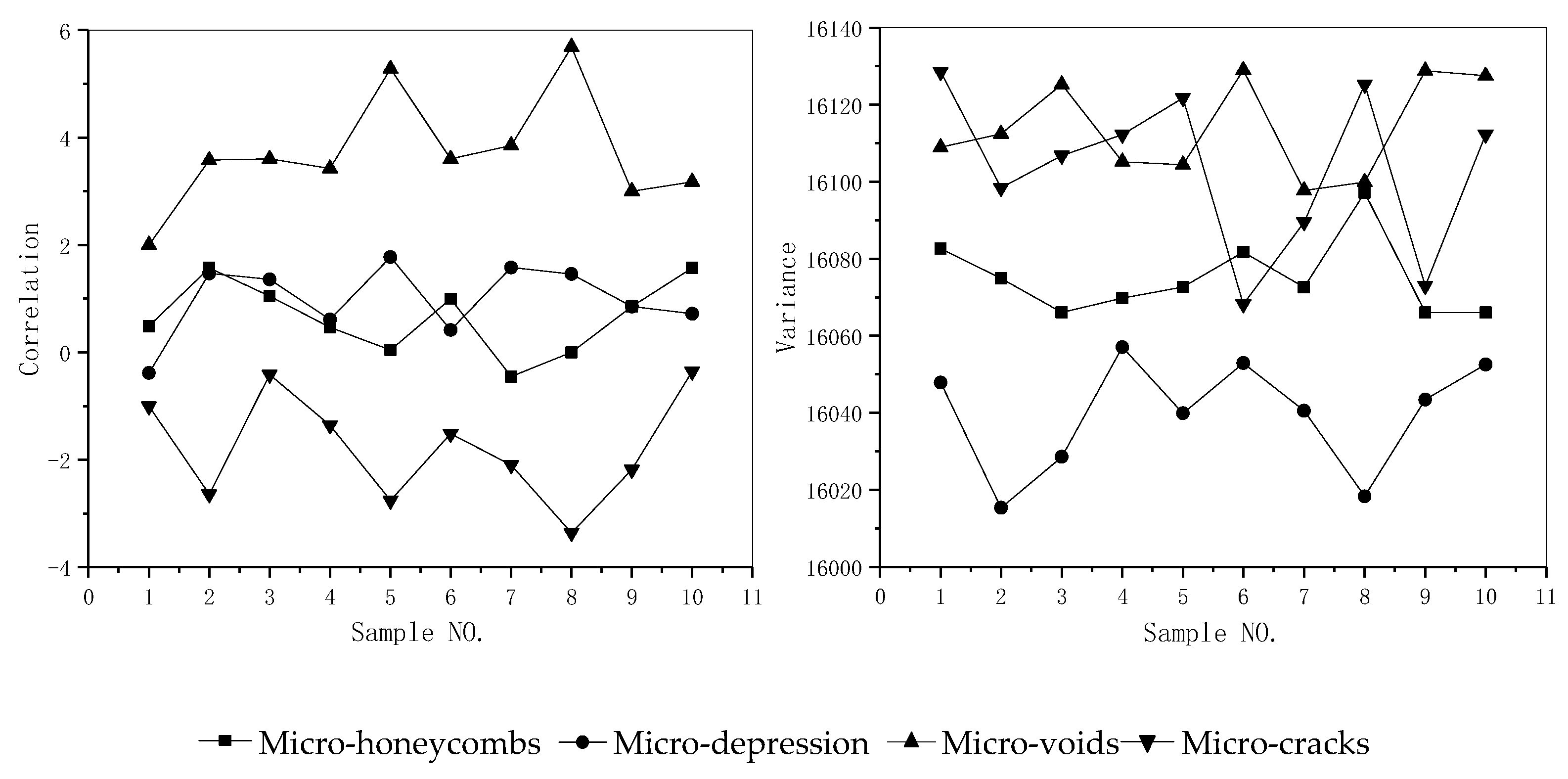
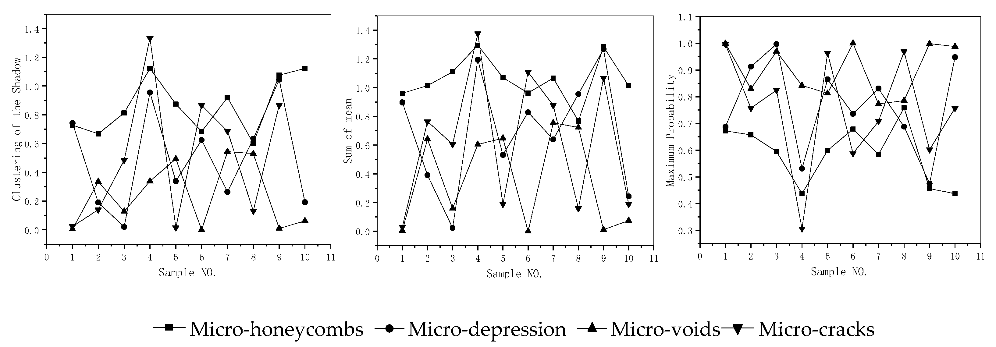
2.2. Feature Parameters
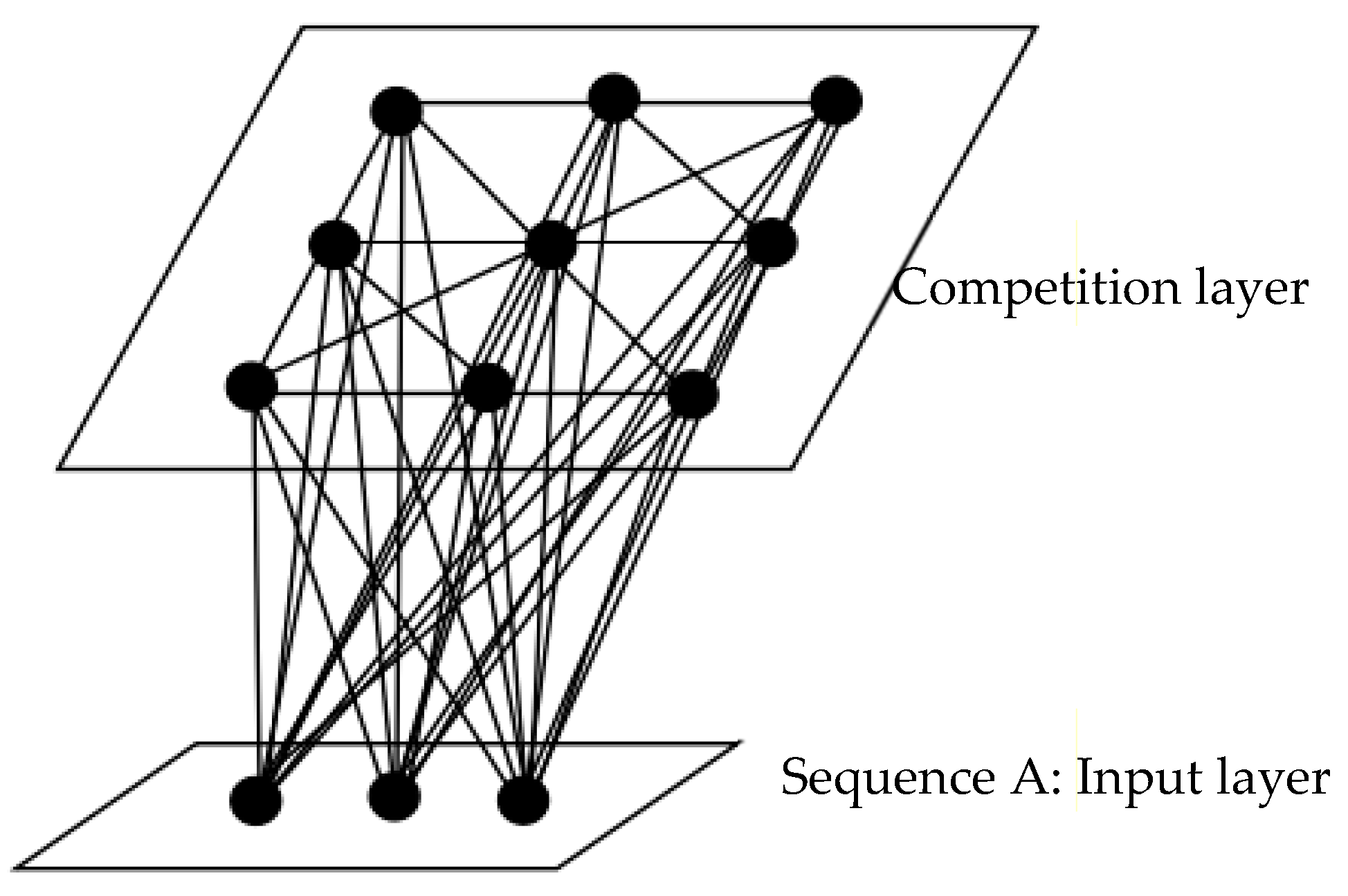
2.3. SOM Networks Model
2.4. Learning Steps
- (i)
- Initialization: Set the [0,1] random value as the initial connection weight between the input neuron and the output neuron. A set, Sj, of outputting neighboring neurons is selected, wherein Sj(0) represents a set of neighboring neurons of neuron j at time t = 0, and Sj(t).
- (ii)
- Set the input of the neural network: Make the sample feature parameters into the following matrix and input them to the SOM network:
- (iii)
- Calculate the Euclidean distance: Input layer neurons, i, into mapping layer neurons’, j, available Euclidean distance, dij, indicated as:In the equation, wij is the weight of the input layer neuron, i, to the mapping layer neuron, j. Wj is the connection weight of the neuron, j, on the mapping layer.
- (iv)
- Obtain the winning neuron: The position of the winning neuron can be obtained by calculating the minimum Euclidean distance between the input vector and the weight vector. When the input vector is X and the winning neuron is denoted by c, the formula is expressed as:where x is the input vector and the winning neuron is labeled c. Wc is the weight of the winning neuron, c. Wi is the connection weight of the neuron, i, on the mapping layer.
- (v)
- Adjust weight: The connection weight of the input neuron and all neurons in the competition neighborhood are corrected by Equation (6):Among them, t is the continuous time, and the learning rate at time t is . or . The value range of is [0,1].
- (vi)
- Determine whether the output result meets the expected requirements: If the result meets the previously set requirements, then end; if not, return to step (ii) to continue.
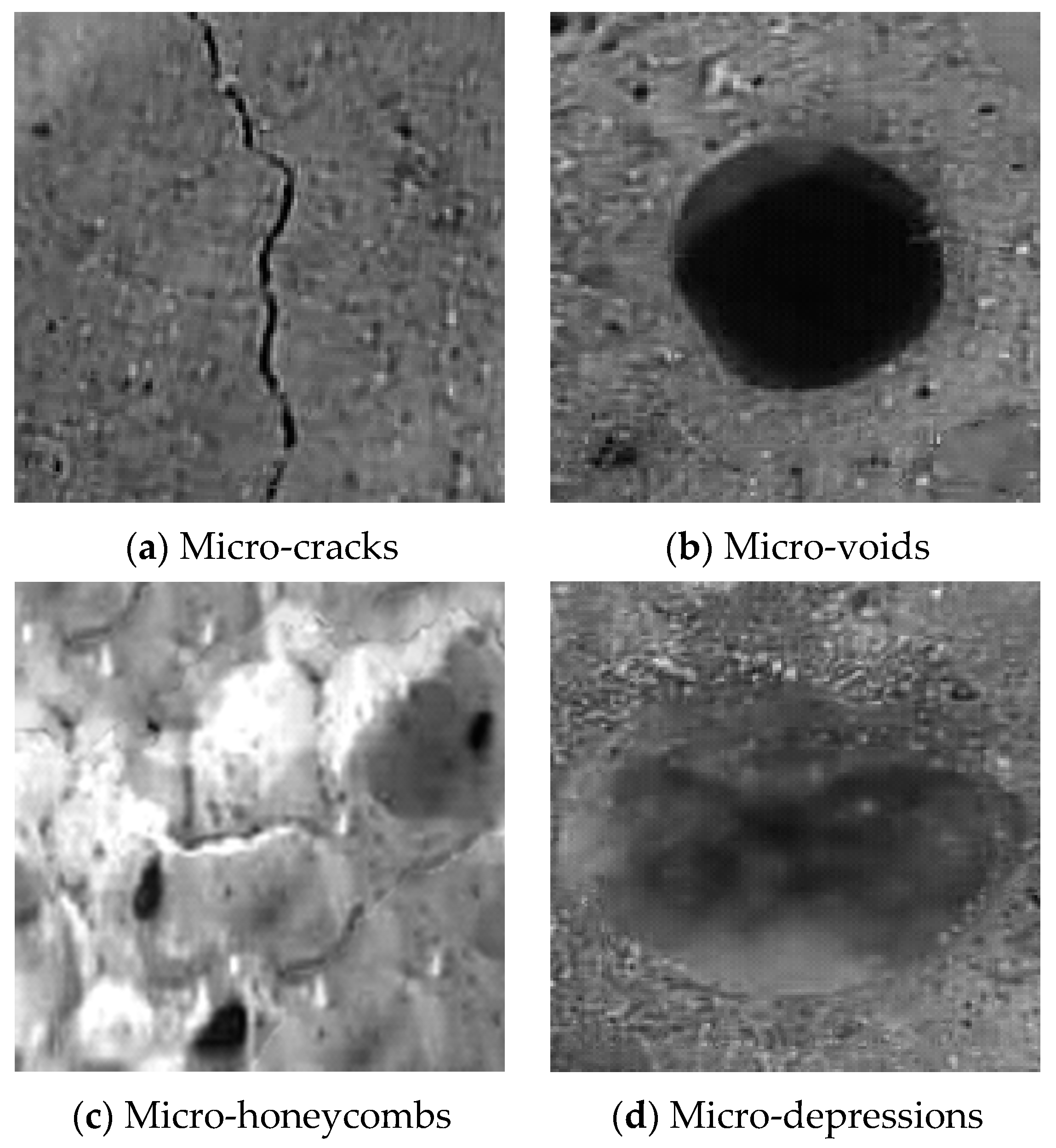
3. Experiment and Result Analysis
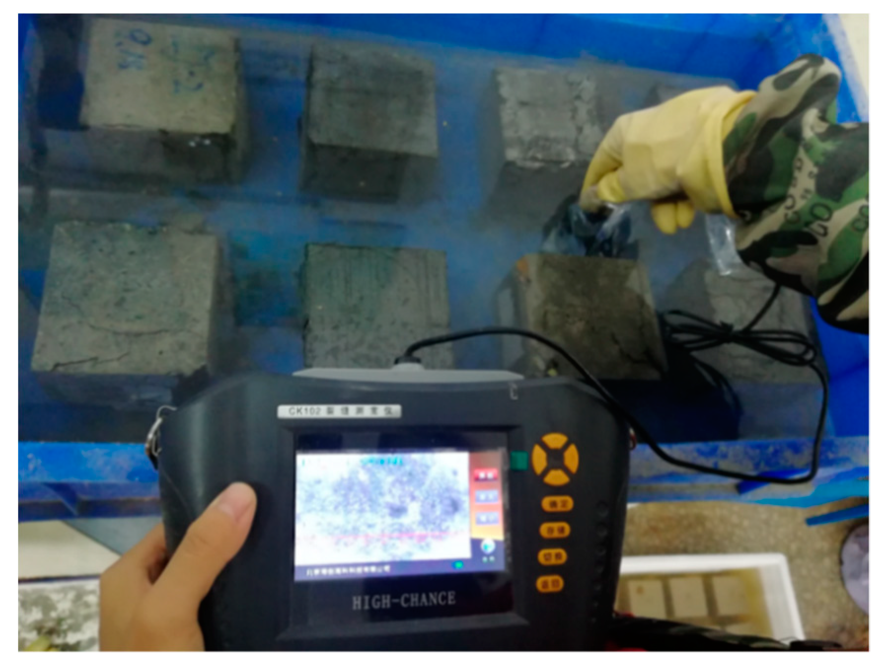
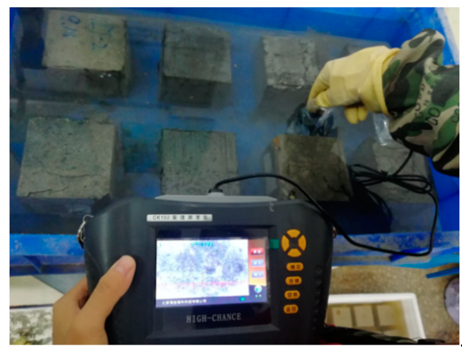
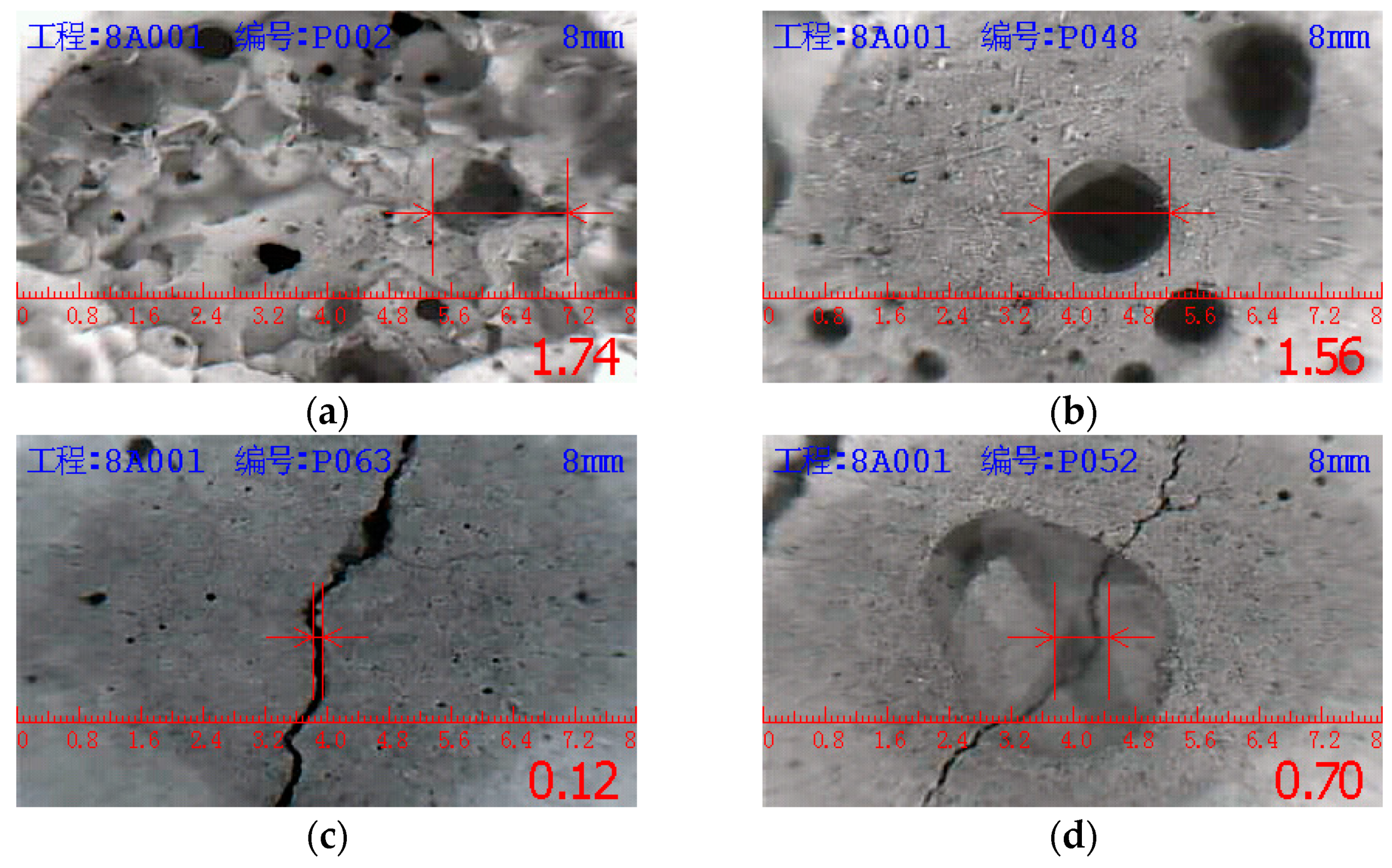
3.1. Image Acquisition and Processing
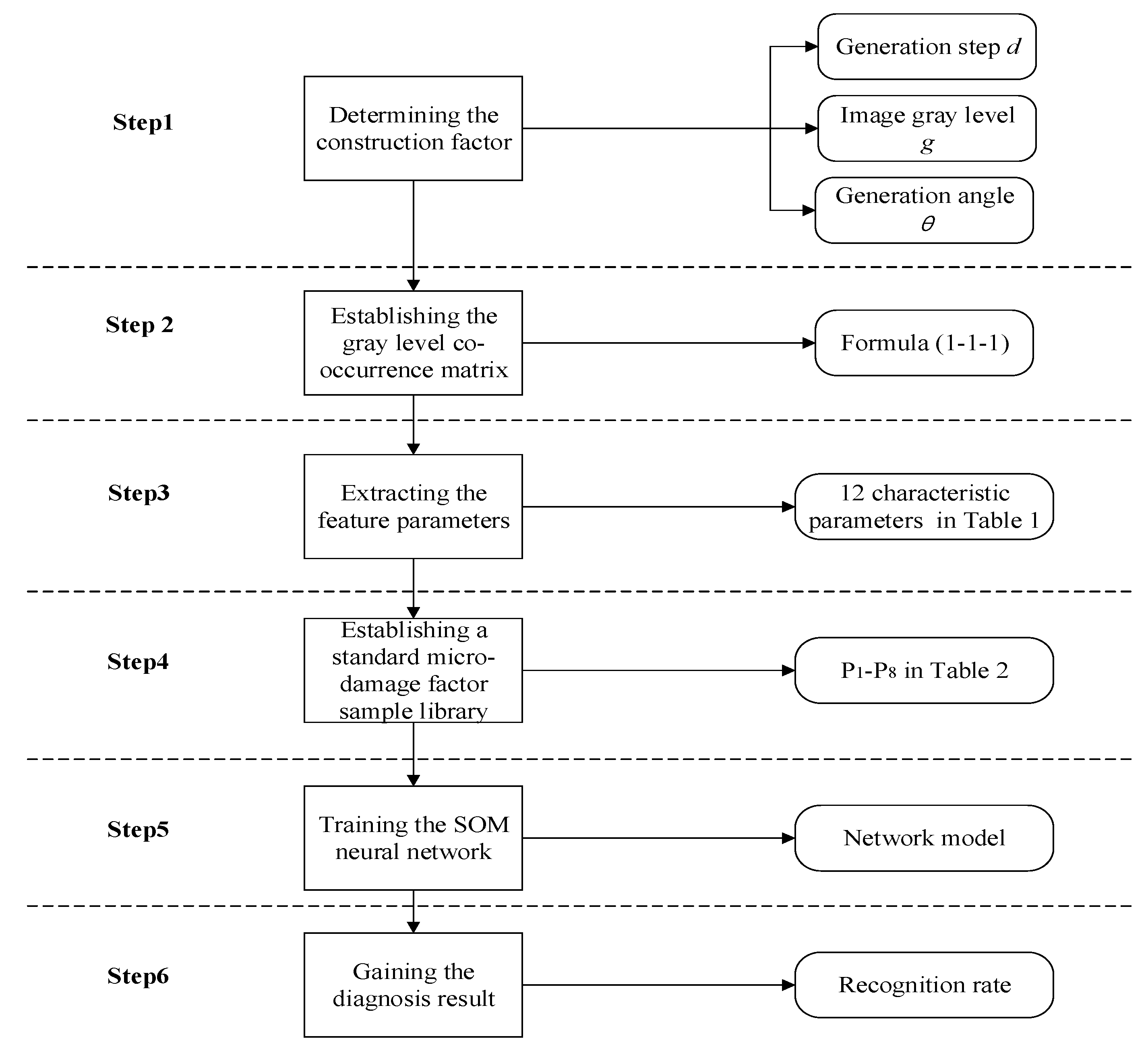
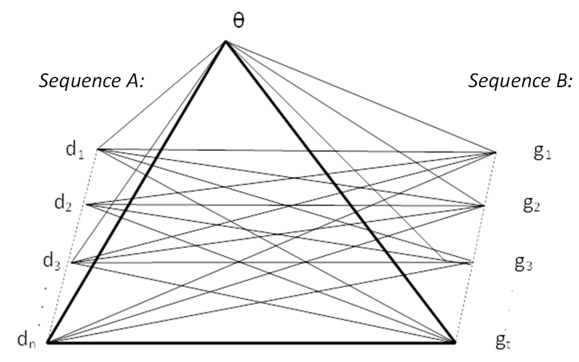
3.2. Triangle Algorithm
- Step 1:
- The initial range of the factor of the generative criterion is determined according to the properties of the micro-damage image.
- Step 2:
- Confirm the generative angle, θ, by the theory of image rotation invariant. In Figure 5, the sequence A is he generative step length, d, g1-gn n is the sequence B image gray level, g, g1-gn.
- Step 3:
- The sequence A is linked to the sequence B, and θ is then joined to sequence A and sequence B, respectively.
- Step 4:
- Extract all dn-θ-gt combinations. Then, a triangular combination can form.
- (1)
- Generative angle, θ: The average of directions of 0°, 45°, 90°, and 135°.
- (2)
- Image gray level: gt = 2m+2, among them, t = m + 2, t is taken as the integer of [1,6].
- (3)
- Generative step length, d: Take the integer of [1,6].
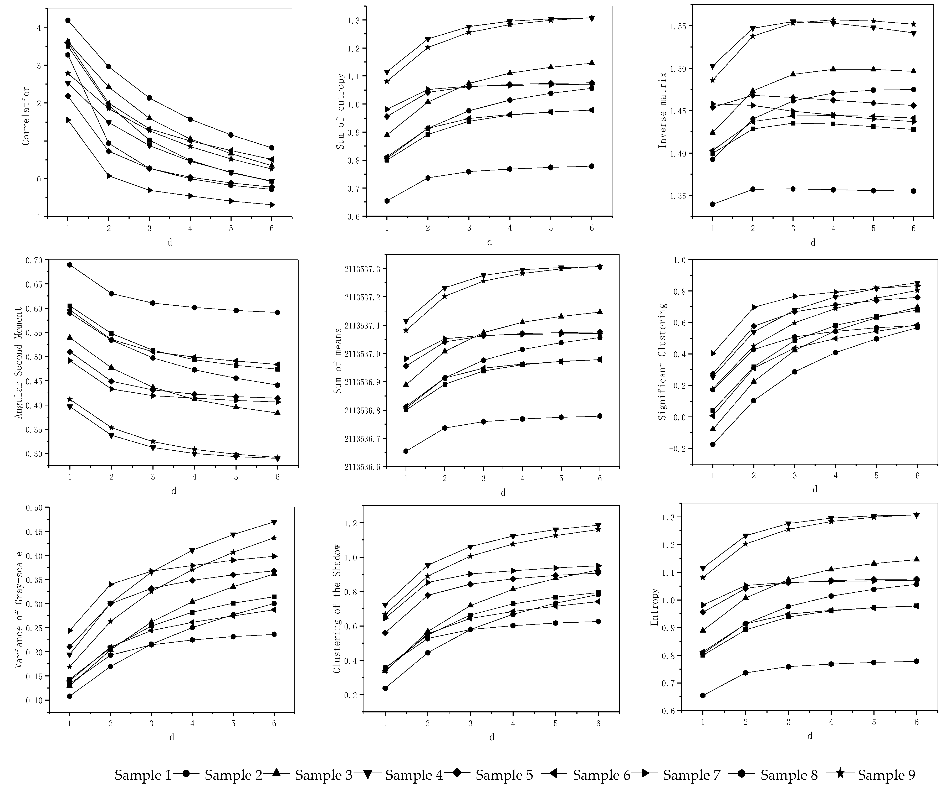
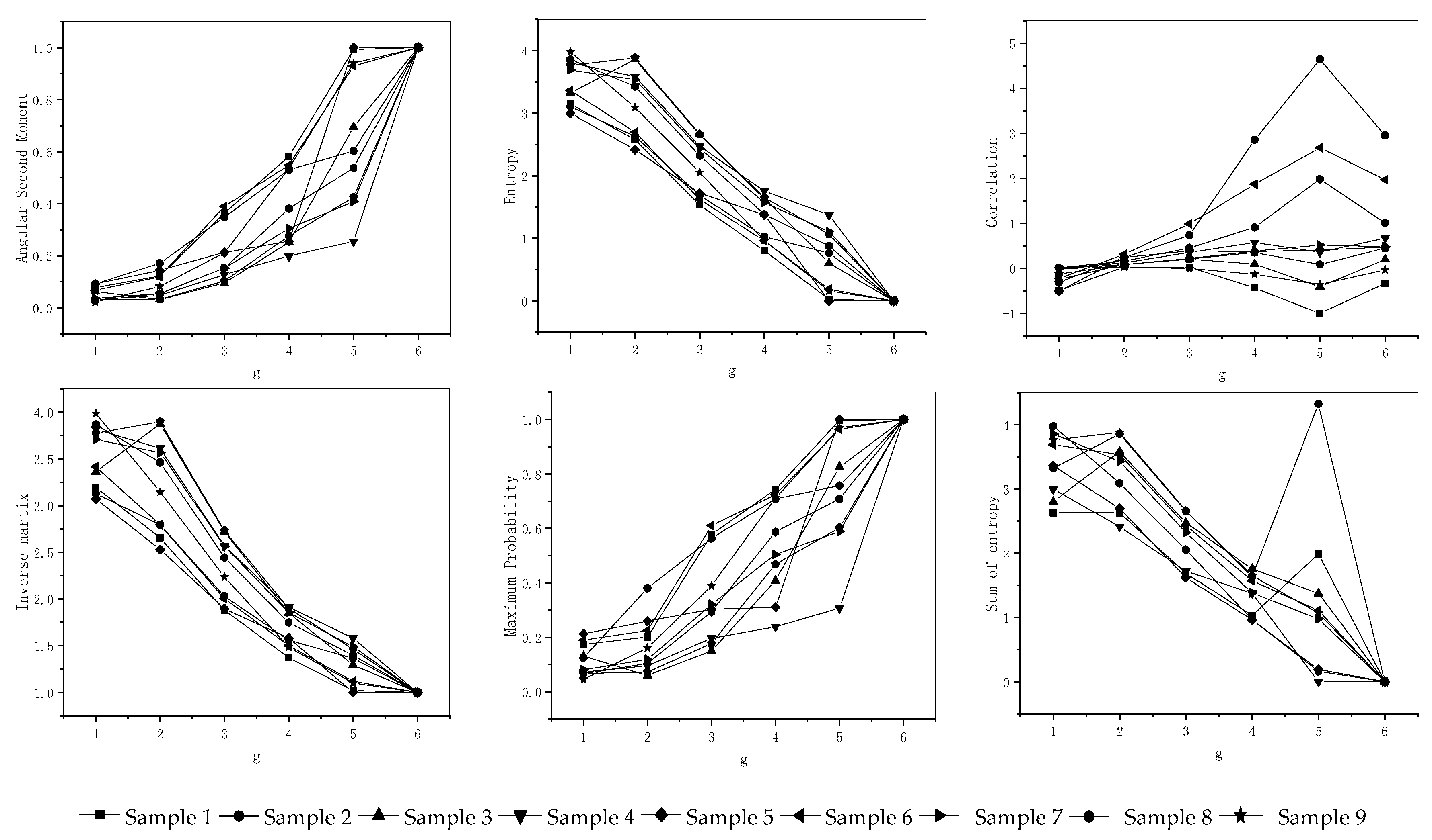
3.3. Optimization of Generative Criterion
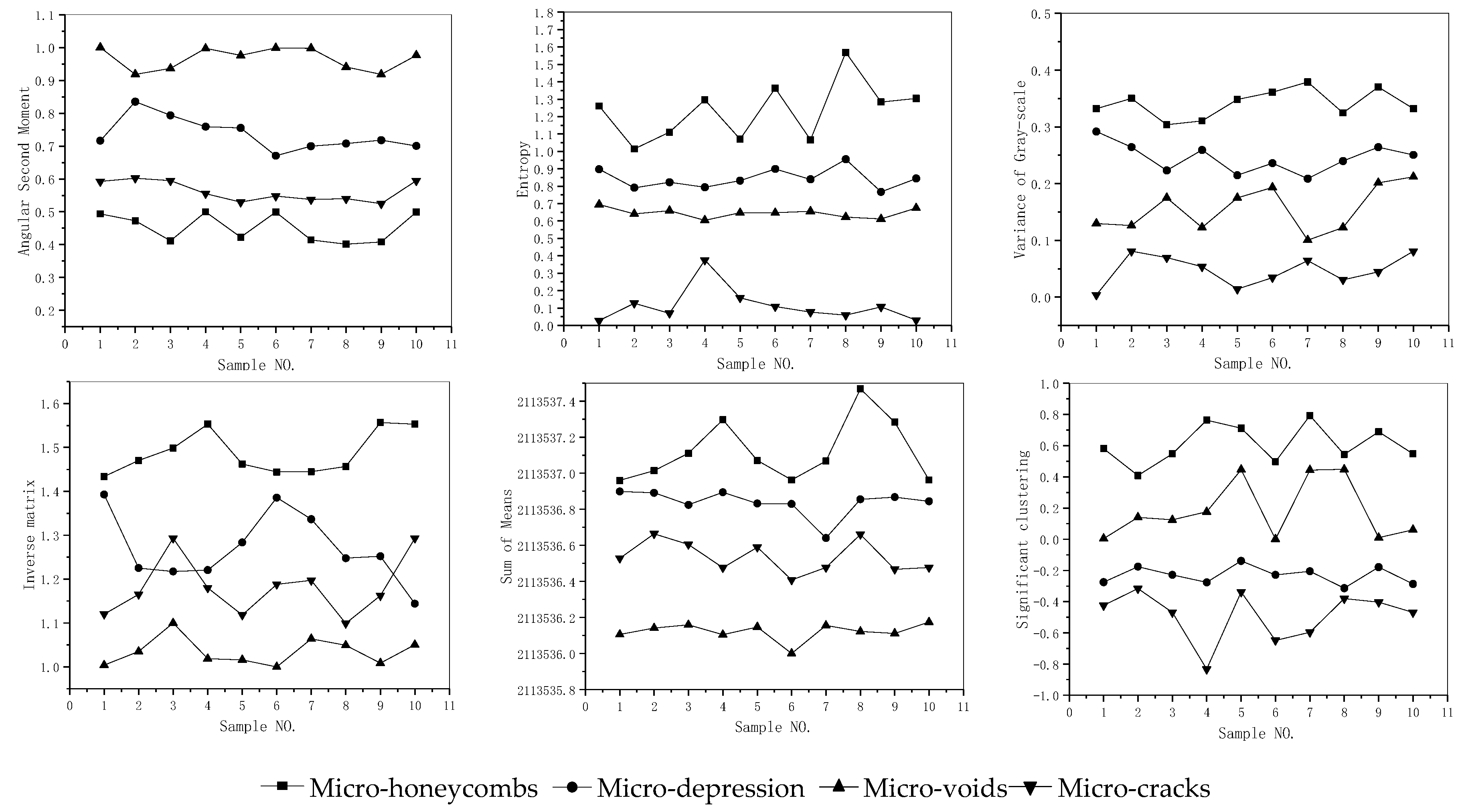
3.4. Establishing a Standard Sample Label
3.5. Training Network Model
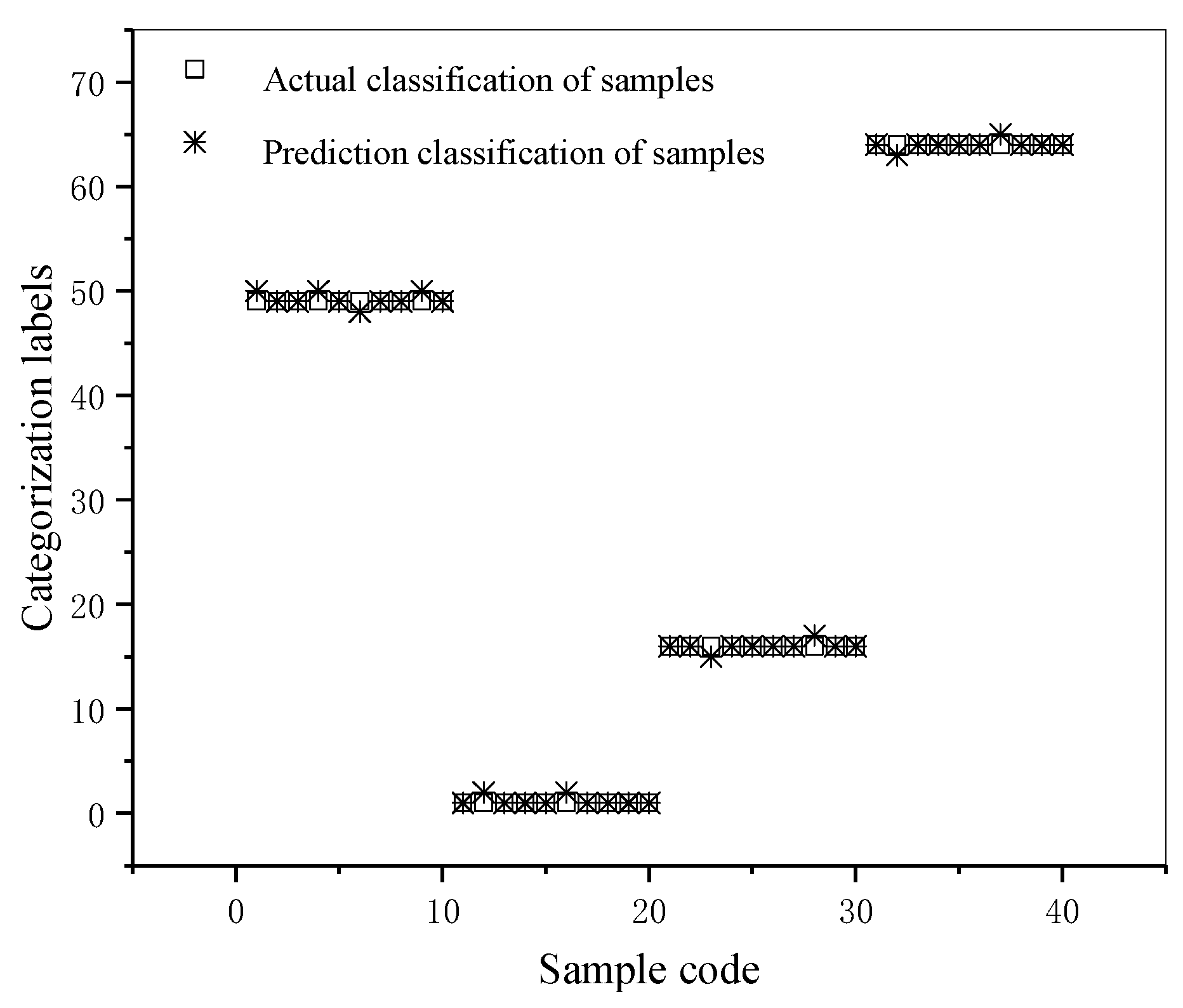
3.6. Application and Validation
4. Conclusions
Author Contributions
Funding
Conflicts of Interest
References
- Farrar, C.R.; Worden, K. An introduction to structural health monitoring. Philos. Trans. A Math. Phys. Eng. Sci. 2010, 365, 303–315. [Google Scholar] [CrossRef] [PubMed]
- Amezquita-Sanchez, J.P.; Adeli, H. Signal Processing Techniques for Vibration-Based Health Monitoring of Smart Structures. Arch. Comput. Methods Eng. 2016, 23, 1–15. [Google Scholar] [CrossRef]
- Bhuiyan, M.Z.A.; Wang, G.; Wu, J.; Cao, J.; Liu, X.; Wang, T. Dependable Structural Health Monitoring Using Wireless Sensor Networks. IEEE Trans. Dependable Secure Comput. 2017, 14, 363–376. [Google Scholar] [CrossRef]
- Park, J.Y.; Lee, J.R. Application of the ultrasonic propagation imaging system to an immersed metallic structure with a crack under a randomly oscillating water surface. J. Mech. Sci. Technol. 2017, 31, 4099–4108. [Google Scholar] [CrossRef]
- Sidibe, Y.; Druaux, F.; Lefebvre, D.; Maze, F.L. Signal processing and Gaussian neural networks for the edge and damage detection in immersed metal plate-like structures. Artif. Intell. Rev. 2016, 46, 289–305. [Google Scholar] [CrossRef]
- Abdeljaber, O.; Avci, O.; Kiranyaz, S.; Gabbouj, M.; Inman, J.M. Real-time vibration-based structural damage detection using one-dimensional convolutional neural networks. J. Sound Vib. 2017, 388, 154–170. [Google Scholar] [CrossRef]
- Bhuiyan, M.Z.A.; Cao, J.; Wang, G. Deploying Wireless Sensor Networks with Fault Tolerance for Structural Health Monitoring. In Proceedings of the IEEE 8th International Conference on Distributed Computing in Sensor Systems, Hangzhou, China, 16–18 May 2012. [Google Scholar]
- Zong, Z.; Zhong, R.; Zheng, P.; Qin, Z.; Liu, Q. Research Progress and Challenges of Bridge Structure Damage Prognosis and Safety Prognosis Based on Health Monitoring. China J. Highw. Transp. 2014, 27, 46–57. [Google Scholar]
- Alavi, A.H.; Hasni, H.; Jiao, P.; Borchani, W.; Lajnef, N. Fatigue cracking detection in steel bridge girders through a self-powered sensing concept. J. Constr. Steel Res. 2017, 128, 19–38. [Google Scholar] [CrossRef]
- Rutkowski, T.A.; Prokopiuk, F. Identification of the Contamination Source Location in the Drinking Distribution System Based on the Neural Network Classifier. IFAC-PapersOnLine 2018, 51, 15–22. [Google Scholar] [CrossRef]
- Chatterjee, S.; Sarkar, S.; Hore, S.; Dey, N.; Ashour, A.S.; Balas, V.E. Particle Swarm Optimization Trained Neural Network for Structural Failure Prediction of Multi-storied RC Buildings. Neural Comput. Appl. 2016, 28, 2005–2016. [Google Scholar] [CrossRef]
- Xu, K.; Deng, Q.; Cai, L.; Ho, S.; Song, G. Damage Detection of a Concrete Column Subject to Blast Loads Using Embedded Piezoceramic Transducers. Sensors 2018, 18, 1377. [Google Scholar] [CrossRef] [PubMed]
- Feng, D.; Feng, M.Q. Experimental validation of cost-effective vision-based structural health monitoring. Mech. Syst. Signal Process. 2017, 88, 199–211. [Google Scholar] [CrossRef]
- Gao, W.; Zhang, G.; Li, H.; Huo, L.; Song, G. A novel time reversal sub-group imaging method with noise suppression for damage detection of plate-like structures. Struct. Control Health Monit. 2017, 25, e2111. [Google Scholar] [CrossRef]
- Cha, Y.J.; Choi, W.; Suh, G.; Mahmoudkhani, S.; Büyüköztürk, O. Autonomous Structural Visual Inspection Using Region-Based Deep Learning for Detecting Multiple Damage Types. Comput. Aided Civ. Infrastruct. Eng. 2017, 33, 731–747. [Google Scholar] [CrossRef]
- Zhu, Z.; German, S.; Brilakis, I. Visual retrieval of concrete crack properties for automated post-earthquake structural safety evaluation. Autom. Constr. 2011, 20, 874–883. [Google Scholar] [CrossRef]
- Molero, M.; Aparicio, S.; Al-Assadi, G.; Casati, M.J.; Hernandez, M.G.; Anaya, J.J. Evaluation of freeze–thaw damage in concrete by ultrasonic imaging. NDT E Int. 2012, 52, 86–94. [Google Scholar] [CrossRef]
- German, S.; Brilakis, I.; Desroches, R. Rapid entropy-based detection and properties measurement of concrete spalling with machine vision for post-earthquake safety assessments. Adv. Eng. Inform. 2012, 26, 846–858. [Google Scholar] [CrossRef]
- Hasni, H.; Alavi, A.H.; Jiao, P.; Lajnef, N. Detection of fatigue cracking in steel bridge girders: A support vector machine approach. Arch. Civ. Mech. Eng. 2017, 17, 609–622. [Google Scholar] [CrossRef]
- Vetrivel, A.; Gerke, M.; Kerle, N.; Nex, F.; Vosselman, G. Disaster damage detection through synergistic use of deep learning and 3D point cloud features derived from very high resolution oblique aerial images, and multiple-kernel-learning. ISPRS J. Photogramm. Remote Sens. 2017, 140, 45–59. [Google Scholar] [CrossRef]
- Yan, Y.; Cheng, L.; Wu, Z.; Yam, L.H. Development in Vibration-Based Structural Damage Detection Technique. Mech. Syst. Signal Process. 2007, 21, 2198–2211. [Google Scholar] [CrossRef]
- Rafiei, M.H.; Adeli, H. A novel unsupervised deep learning model for global and local health condition assessment of structures. Eng. Struct. 2018, 156, 598–607. [Google Scholar] [CrossRef]
- Cha, Y.J.; Choi, W.; Büyüköztürk, O. Deep Learning-Based Crack Damage Detection Using Convolutional Neural Networks. Comput. Aided Civ. Infrastruct. Eng. 2017, 32, 361–378. [Google Scholar] [CrossRef]
- Liu, L.; Fieguth, P.; Guo, Y.; Wang, X.; Pietikäinen, M. Local binary features for texture classification: Taxonomy and experimental study. Pattern Recognit. 2017, 62, 135–160. [Google Scholar] [CrossRef]
- Malegori, C.; Franzetti, L.; Guidetti, R.; Casiraghi, E.; Rossi, R. GLCM, an image analysis technique for early detection of biofilm. J. Food Eng. 2016, 185, 48–55. [Google Scholar] [CrossRef]
- Maddalena, L.; Petrosino, A. A Self-Organizing Approach to Background Subtraction for Visual Surveillance Applications. IEEE Trans. Image Process. 2008, 17, 1168–1177. [Google Scholar] [CrossRef]
- Li, X.; Zhu, D. An Adaptive SOM Neural Network Method to Distributed Formation Control of a Group of AUVs. IEEE Trans. Ind. Electron. 2018, 65, 8260–8270. [Google Scholar] [CrossRef]
- Merainani, B.; Rahmoune, C.; Benazzouz, D.; Ould-Bouamama, B. A novel gearbox fault feature extraction and classification using Hilbert empirical wavelet transform, singular value decomposition, and SOM neural network. J. Vib. Control 2017, 24, 2512–2531. [Google Scholar] [CrossRef]
- Li, Y.; Yao, X.; Li, W.; Li, C. Model Optimization of Wood Property and Quality Tracing Based on Wavelet Transform and NIR Spectroscopy. Spectrosc. Spectr. Anal. 2018, 38, 1384–1392. [Google Scholar]
- Kamruzzaman, M.; Elmasry, G.; Sun, D.W.; Allen, P. Non-destructive assessment of instrumental and sensory tenderness of lamb meat using NIR hyperspectral imaging. Food Chem. 2013, 141, 389–396. [Google Scholar] [CrossRef]
- Raju, P.; Rao, V.M.; Rao, B.P. Optimal GLCM combined FCM segmentation algorithm for detection of kidney cysts and tumor. Multimed. Tools Appl. 2019, 78, 18419–18441. [Google Scholar] [CrossRef]
- Ancy, C.A.; Nair, L.S. Tumour Classification in Graph-Cut Segmented Mammograms Using GLCM Features-Fed SVM. Intell. Eng. Inform. 2018, 695, 197–208. [Google Scholar]
- Chen, J.; Chen, Z.; Chi, Z.; Fu, H. Facial Expression Recognition in Video with Multiple Feature Fusion. IEEE Trans. Affect. Comput. 2018, 9, 38–50. [Google Scholar] [CrossRef]
- Oliveira, R.B.; Papa, J.P.; Pereira, A.S.; Tavares, J.M.R.S. Computational methods for pigmented skin lesion classification in images: Review and future trends. Neural Comput. Appl. 2016, 29, 613–636. [Google Scholar] [CrossRef]
- Torres-Alegre, S.; Fombellida, J.; Piñuela-Izquierdo, J.A.; Andina, D. AMSOM: Artificial metaplasticity in SOM neural networks—Application to MIT-BIH arrhythmias database. Neural Comput. Appl. 2018, 1–8. [Google Scholar] [CrossRef]
- Rodriguez-Galiano, V.F.; Chica-Olmo, M.; Abarca-Hernandez, F.; Atkinson, P.M.; Jeganathan, C. Random Forest classification of Mediterranean land cover using multi-seasonal imagery and multi-seasonal texture. Remote Sens. Environ. 2012, 121, 93–107. [Google Scholar] [CrossRef]
- Rokach, L. A survey of Clustering Algorithms. Data Mining Knowl. Discov. Handb. 2009, 16, 269–298. [Google Scholar]
- Vesanto, J.; Alhoniemi, E. Clustering of the self-organizing map. IEEE Trans. Neural Netw. 2000, 11, 586–600. [Google Scholar] [CrossRef]
- Kohonen, T. Essentials of the self-organizing map. Neural Netw. 2013, 37, 52–65. [Google Scholar] [CrossRef]


| NO. | Parameters | Calculation Formulas | Texture Characteristic |
|---|---|---|---|
| T1 | Angular second moment | The uniformity of gray distribution and degree of texture. | |
| T2 | Sums of average | The change of brightness. | |
| T3 | Sums of variance | Texture period size. | |
| T4 | Maximum probability | The distribution of the main texture. | |
| T5 | Sums of entropy | Texture complexity. | |
| T6 | Variance | Texture periodicity. | |
| T7 | Variance of grayscale | Texture distribution. | |
| T8 | Correlation | The main direction of the texture. | |
| T9 | Inverse matrix | Local texture changes. | |
| T10 | Cluster shadow | Texture uniformity. | |
| T11 | Significant clustering | Texture uniformity. | |
| T12 | Entropy | Texture randomness. |
| Damage Type | P1 | P2 | P3 | P4 | P5 | P6 | P7 | P8 |
|---|---|---|---|---|---|---|---|---|
| Micro-honeycombs | 0.45219 | 1.23347 | 0.341173 | 0.659015 | 1.487459 | 16074.99305 | 0.6085123 | 2113537.15 |
| Micro-depressions | 0.735626 | 0.844082 | 0.245272 | 0.986124 | 1.270514 | 16039.67163 | −0.23044 | 2113536.83 |
| Micro-voids | 0.966008 | 0.645785 | 0.155829 | 3.719458 | 1.034531 | 16113.92133 | 0.185468 | 2113536.14 |
| Micro-cracks | 0.561931 | 0.114353 | 0.047756 | −1.768837 | 1.1816 | 16103.60313 | −0.487734 | 2113536.55 |
| Parameters | Value | |||||||
|---|---|---|---|---|---|---|---|---|
| Input Layer Node | x1 | x2 | x3 | x4 | x5 | x6 | x7 | x8 |
| P1 | P2 | P3 | P4 | P5 | P6 | P7 | P8 | |
| Weight | 0.125 | |||||||
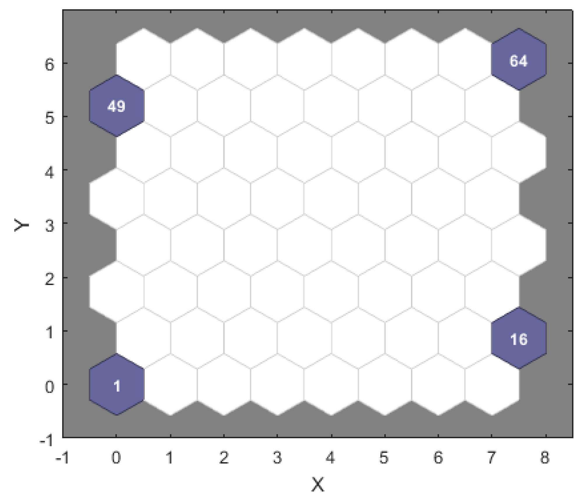
| Neighborhood shape | Hexagon, R = 3 | |||||||
| Neurons | 64 | |||||||
| Training steps | 10, 50, 100, 200, 500,1000 | |||||||
| Number of Training Steps | Micro-Honeycombs | Micro-voids | Micro-depressions | Micro-cracks | Clustering Result |
|---|---|---|---|---|---|
| 10 | 55 | 37 | 37 | 55 | 50% |
| 50 | 43 | 37 | 37 | 55 | 75% |
| 100 | 43 | 1 | 37 | 37 | 75% |
| 200 | 49 | 1 | 16 | 64 | 100% |
| 500 | 49 | 1 | 16 | 64 | 100% |
| 1000 | 49 | 1 | 16 | 64 | 100% |
| Damage Type | Sample Classification Number | Classification Accuracy |
|---|---|---|
| Micro-honeycombs | 36, 41, 42, 43, 44, 49, 50, 51, 52, 57, 58, 59 | 80% |
| Micro-voids | 1, 2, 3, 4, 9, 10, 17, 18, 19, 20, 25, 26, 27, 33, 34, 35 | 93.33% |
| Micro-depressions | 5, 6, 7, 8, 11, 12, 13, 14, 15, 16, 21, 22, 23, 24, 29 | 100% |
| Micro-cracks | 30, 31, 32, 38, 39, 40, 45, 46, 47, 48, 54, 55, 56, 61, 62, 63, 64 | 86.66% |
| Unknown situation | 53, 60 | - |
| 28 | - | |
| 37 | - |
| Damage Type | Sample Number |
|---|---|
| Micro-honeycombs | 1–10 |
| Micro-voids | 11–20 |
| Micro-depressions | 21–30 |
| Micro-cracks | 31–40 |
© 2019 by the authors. Licensee MDPI, Basel, Switzerland. This article is an open access article distributed under the terms and conditions of the Creative Commons Attribution (CC BY) license (http://creativecommons.org/licenses/by/4.0/).
Share and Cite
Li, K.; Wang, J.; Qi, D. An Intelligent Warning Method for Diagnosing Underwater Structural Damage. Algorithms 2019, 12, 183. https://doi.org/10.3390/a12090183
Li K, Wang J, Qi D. An Intelligent Warning Method for Diagnosing Underwater Structural Damage. Algorithms. 2019; 12(9):183. https://doi.org/10.3390/a12090183
Chicago/Turabian StyleLi, Kexin, Jun Wang, and Dawei Qi. 2019. "An Intelligent Warning Method for Diagnosing Underwater Structural Damage" Algorithms 12, no. 9: 183. https://doi.org/10.3390/a12090183
APA StyleLi, K., Wang, J., & Qi, D. (2019). An Intelligent Warning Method for Diagnosing Underwater Structural Damage. Algorithms, 12(9), 183. https://doi.org/10.3390/a12090183