Variational Calculus Approach to Optimal Interception Task of a Ballistic Missile in 1D and 2D Cases

Abstract

The paper presents the application of variational calculus to achieve the optimal design of the open-loop control law in the process of anti-ballistic missile interception task. It presents the analytical results in the form of appropriate Euler–Lagrange equations for three different performance indices, with a simple model of the rocket and the missile, based on the conservation of momentum principle. It also presents the software program enabling rapid simulation of the interception process with selected parameters, parametric analysis, as well as easy potential modification by other researchers, as it is written in open code as m-function of Matlab.

1. Introduction

Interception of ballistic missiles has been a research topic for years. Calculation of interception trajectories is usually performed off-line by using two-point boundary-value problem formulation. The paper [1] employs the proposed guidance law in real-world conditions, where interception trajectories are sought in $R^6$, comprising of: three NED (north-east-down) coordinates, speed, path angle and heading of the interceptor. This usually calls for the use of optimization techniques to obtain the reference trajectories to follow. In [2], there are four different guidance laws considered, showing that the interception of the missile is possible if one has perfect measurements and accurate estimation of the target maneuvers. To obtain the optimal interception point, one can use multiple approaches, ranging from classical variational calculus as in this paper, or others, such as metaheuristics, e.g., a genetic algorithm, see [3], which is used there to establish the optimal interception point, minimizing certain functional. The functional may refer to flight time of the intercepting missile, or distance between the interceptor and the ballistic missile. Guidance of an intercepting rocket is a problem which has multiple solutions. One can distinguish passive and active guidance approaches [4]. Several types of active guidance methods can be distinguished:

• line of sight guidance (also called a two-point guidance), where the intercepting rocket always points to the target,
• deviated pursuit, where the intercepting missile points ahead of the target,
• proportional navigation, where the line of sight angle of the target is estimated,
• optimal guidance by minimizing a certain functional.

Among the last, one can consider many approaches, such as LQR [5] embedded into variational calculus framework, LQI (LQ integrated) control law [6], applied to linearized systems, predictive control and nonlinear predictive control, which fall into the optimization strand [7], or performance-based approaches to PID tuning, [8]. This paper adopts the optimization technique to generate the optimal open-loop control signal to reach the desired point minimizing a certain performance index. A more comprehensive view on a general framework of a ballistic missile defense systems, comprising of a launcher and a radar, please refer to [9]. Another study of tracking a ballistic missile can also be found in [10].

Optimization techniques have been developed for ages—it was in 17th century when such mathematicians as Leibnitz, Bernoulli, Newton of d’Hospital pushed their horizons further. They are required in production processes, business/management, or in military applications, since everybody is interested in gathering as much as possible, at the least expense, in the shortest time, etc. The aim of this paper is to use this approach in the optimal interception problem of a ballistic rocket with a known trajectory, using the intercepting missile.

As has been already remarked, an optimization approach is attractive in many areas, and can include, e.g., quadratic cost function in an unbounded problem, leading to an easy solution. In real world applications, however, constraints are ubiquitous, and need to be taken into consideration during the optimization process. In this work, optimization is based on variational calculus that could be, e.g., presented as the problem of finding, among all the continuous functions $x\left(t\right)$, the one that satisfies terminal conditions [11]:

$$x\left(t_0\right)=x_0,x\left(t_f\right)=x_f,$$

(1)

achieving local extremum of the functional

$$J\left(x\right)={\int }_{t_0}^{t_f}f(f(t,x\left(t\right),\dot{x}\left(t\right))dt.$$

(2)

The latter task has fixed terminal conditions, and the necessary condition of existence of such an extremum is satisfying the Euler–Lagrange (E–L) equation

$$\frac{\partial f}{\partial x}-\frac{d}{dt}\left(\frac{\partial f}{\partial \dot{x}}\right)=0.$$

(3)

From now on, whenever applicable without misunderstandings, the time indexes will be omitted. In the case of a variable initial point lying on the curve $\varphi \left(x\right)$, the function $x\left(t\right)$ is sought that crosses $(t_0,x_0)$ and intersects $\varphi \left(x\right)$ at time $t_f$. This function satisfies, in addition to E–L equation, the following transversality conditions:

$$\begin{array}{c}\hfill f(t_0,x,\dot{x})={\left.\left[({\dot{x}}_0-\dot{\varphi })\frac{\partial f}{\partial \dot{x}}\right]\right|}_{t=t_0},\end{array}$$

(4)

$$\begin{array}{c}\hfill f(t_f,x,\dot{x})={\left.\left[({\dot{x}}_0-\dot{\varphi })\frac{\partial f}{\partial \dot{x}}\right]\right|}_{t=t_f}.\end{array}$$

(5)

If the functional depends on $\underline{x}$, then the necessary conditions are formed as a set of E–L equations. In the considered interception task, $\varphi$ might depict the route traced by the nuclear train from what the missile is launched at $t_0$, or the path of the rocket to be hit at $t_f$.

Finally, when constraints are present and can be put in the form $\underline{g}(t,x,u)=\underline{b}$, where u denotes the control signal, and $\underline{g}$ is some function satisfying continuity conditions, the functional can be put in the form

$$J\left(x\right)={\int }_{t_0}^{t_f}\left(f(t,x,\dot{x},u,\dot{u})+{\underline{\lambda }}^T\left(\underline{b}-\underline{g}(t,x,u)\right)\right)dt.$$

(6)

The variational approach presented above will be adopted for finding optimal control signals of a missile to intercept a ballistic rocket, for which model and parameters will be presented in the next Section. The anti-ballistic missile is abbreviated in the paper as ABM, and is usually a surface-to-air missile designed to counter ballistic missiles [12,13].

As optimal interception tasks have already been solved and considered in the literature, presenting various scenarios and solutions, though as a set of pure results only, and form a continuously-developed research field, this paper presents the software in open text which can be used not only to simulate interception task, taking multiple system parameters into account during analysis, but also to perform parametric analysis on selected performance indices. All the issues will be addressed in the paper, which is the main motivation and contribution of this work.

2. Models of an Intercepting Missile and Ballistic Rocket

2.1. Simplified Intercepting Missile Model (1D)

Prior to giving a model of a rocket the question of model accuracy should be addressed. It would seem advantageous to find the most accurate model, but in such a case, computer calculations would take too much time, and mathematical description would disable any actions. The model should be simplified enough to mirror the dynamics of the missile, but not be oversimplified.

The missile is assumed to move on the basis of propulsion force, where gases leaving the rocket move it in the opposite direction [14,15,16]. In order to enable mathematical description, the momentum conservation rule has been used, which states that the total momentum of the rocket ($p_{\mathrm{rocket}}\left(t\right)+p_{\mathrm{gas}}\left(t\right)$) always adds to zero, where

$$p_{\mathrm{gas}}\left(t\right)=mv\left(t\right),$$

(7)

with m being the mass of the rocket, and $v\left(t\right)$ being its velocity. The effect of the drag force is harder to quantify, nevertheless, since in many important applications drag effects are very small, the drag force is omitted here. Potential drag effects, where the density of air changes with altitude, usually result in equations that are impossible to be integrated analytically (numerical integrations are needed), and leads to, in typical flight conditions of a 12,000 $\mathrm{kg}$ rocket flying at $700\mathrm{m}/\mathrm{s}$, a drag force at the level of $2\%$ of gravity force.

The considered control system should work in the following way: the control signal $w\left(t\right)$ is the momentum of the gas, which when divided by m gives the velocity of the rocket. By integrating this velocity one can obtain information about the position of the rocket that should be compared with the information about the trajectory of the rocket that must be intercepted. The location is measured by a sensor, represented by pure feedback gain, and this signal should be subtracted from the reference signal w to obtain tracking error. The controller itself is not needed, since the open-loop control signal will be obtained as the result of optimization.

Assuming that $m_r$ is the mass of he missile, $k_2$ is the gain in the inner feedback loop of the rocket, $w\left(t\right)$ is the reference signal (optimized input signal to the control system), and $y\left(t\right)$ is its output, one can propose the following model with $k_1=\frac{1}{m_r}$ (see Figure 1):

$$G\left(s\right)=\frac{Y\left(s\right)}{W\left(s\right)}=\frac{\frac{k_1}{s}}{1+\frac{k_1{k}_2}{s}}=\frac{\frac{1}{k_2}}{1+\frac{1}{k_1{k}_2}s}=\frac{k}{1+sT}.$$

(8)

The time constant of the rocket is assumed to be approximately several minutes, and its mass approximately $1000\mathrm{kg}$ [13,17,18].

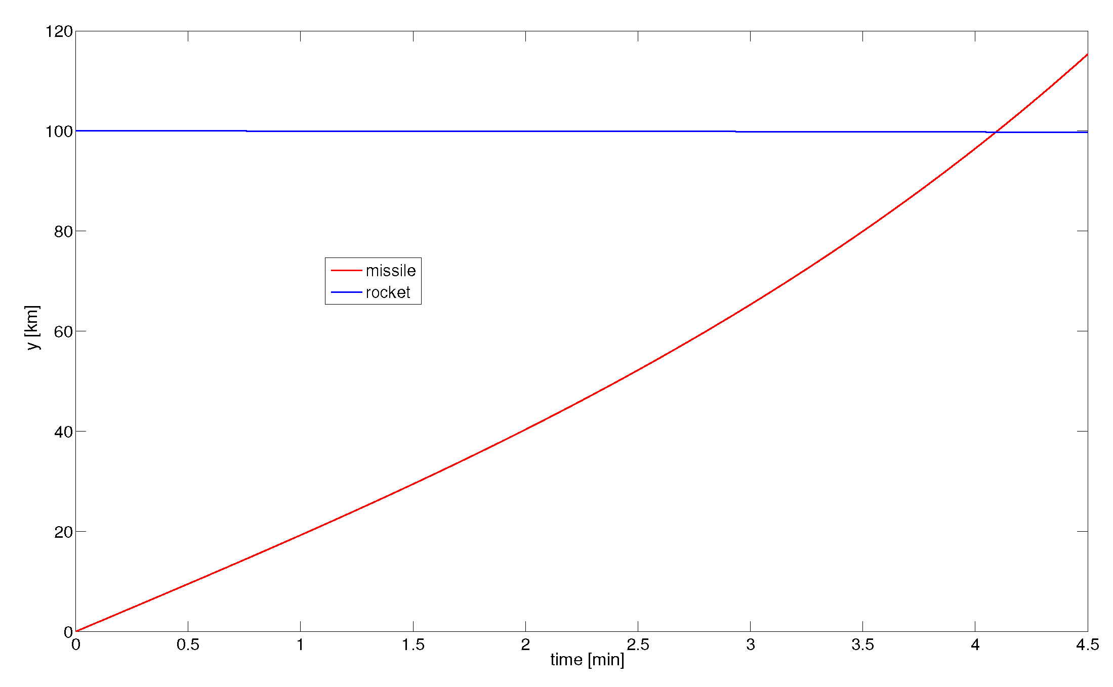
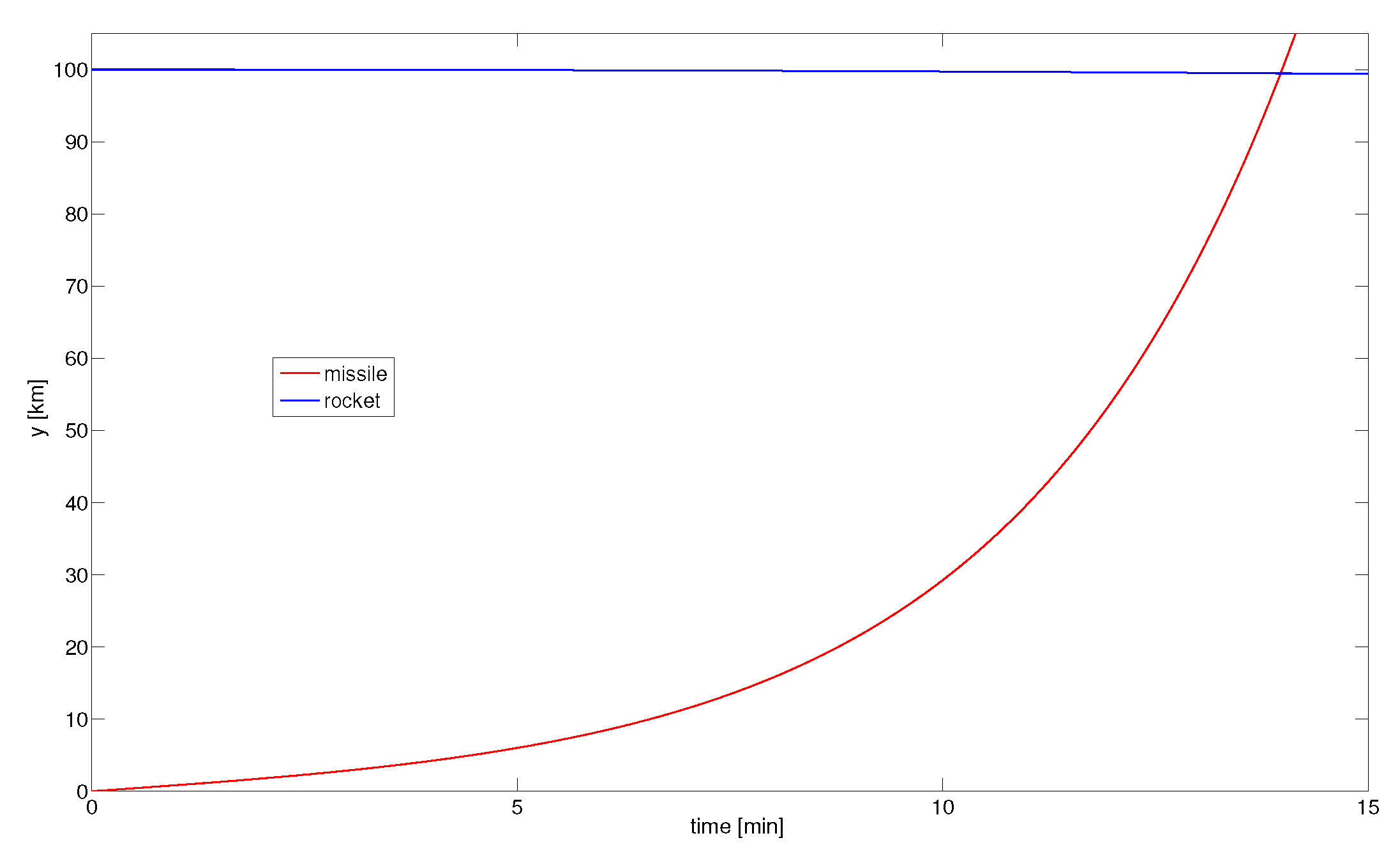
2.2. Simplified Rocket Model (1D)

Typical ballistic rocket is flying approximately horizontally the middle phase of its flight, plotting parabolic ∩-shaped function. The parabola should have a flat graph with some maximum attitude assumed, as in this paper, i.e., $100\mathrm{km}$. Typical parameters of the intercepting missiles are given in the

Table 1. Standard parameters of interception missiles.

Parameter	Value
maximum attitude	80 ÷ 100 km
linear velocity	2000 ÷ 6000 kmph
mass	1000 ÷ 10,000 kg
time of flight	20 ÷ 40 mins
range	100 ÷ 5000 km

and

Table 2. Selected parameters of sample interception missiles.

Parameter	Iskander	Shahab 3	MGM-31B Per/II
country	Russia	Iran	USA
mass	3800 kg	900 kg	7400 kg
max. vel.	6000 kmph	5500 kmph	3000 kmph
range	500 km	2100 km	1800 km

[12].

The trajectory of the rocket might be defined by the following canonical quadratic function

$$\phi =a{(t-p)}^2+q,$$

(9)

where $p\left[\mathrm{h}\right]$ is the time in which the missile reaches its maximum altitude, a is the slope, and $q\left[\mathrm{km}\right]$ is the maximum altitude [14,16].

The missile used to intercept the ballistic rocket does not have any information about the time when the latter has been launched, thus $t=0$ denotes the launch time of the intercepting missile. Assuming, as an example, that $p=0.25\mathrm{h}$ with arbitrary chosen $a=-10$, the default canonical ballistic rocket equation in 1D becomes

$$\phi \left(t\right)=-10{(t-0.25)}^2+100.$$

(10)

Such a 1D case can be interpreted as a situation when the interception takes place directly above the place of installation of intercepting rockets, below expected ballistic missile trajectory.

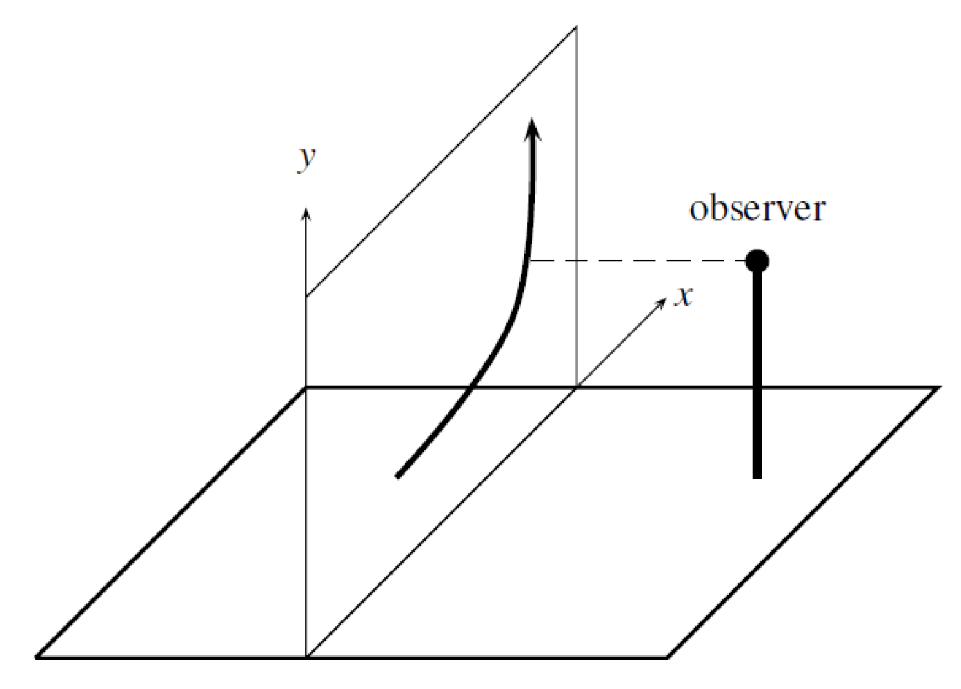
2.3. Intercepting Missile Model (2D)

The 2D task is the actual point of interest, where translation of the missile takes place in a two-dimensional space (distance x vs. altitude y). It is assumed that the observer is in parallel to the hyperplane on which the translation of the missile takes place, as well as the translation of the rocket, and their observation angle is the right angle, as depicted in Figure 2.

By assuming a specified localization of the observer, there is no need to present the translation in 3D space, thus z axis information can be omitted.

Generalizing the previous 1D momentum equation to the 2D case [15],

$$p_{\mathrm{total}}=m(v_x+v_y)=m{v}_x+m{v}_y=p_x+p_y,$$

(11)

where velocity vector $\underline{v}$ is decomposed into x- and y-components.

With the base vectors ${\underline{e}}_1$ and ${\underline{e}}_2$, the momentum $\underline{p}=p_x{\underline{e}}_1+p_y{\underline{e}}_2$.

2.4. Rocket Model (2D)

The ballistic rocket that should be intercepted is assumed to move as in the 1D case on a paraboloid, and its range is assumed to be $2000\mathrm{km}$ by default and maximum height in y coordinate—$100\mathrm{km}$, i.e., it is a medium-range missile according to the American division or Russian classification [12], see

Table 3. Missile types (American).

Range	Missile Type
150 ÷ 300 km	tactical ballistic missile
300 ÷ 1000 km	short-range ballistic missile
1000 ÷ 3500 km	medium-range ballistic missile
3500 ÷ 5500 km	intermediatet-range ballistic missile
over 5500 km	intercontinental ballistic missile

and

Table 4. Missile types (Russian).

Range	Missile Type
below 50 km	tactical missile
50 ÷ 300 km	operationa-tactial missile
300 ÷ 500 km	operational missile
500 ÷ 1000 km	operation-strategic missile
over 1000 km	strategic missile

.

Among American ABMs currently used one can find: MIM-104 Patriot (PAC-1 and PAC-2), U.S. Navy Aegis combat system using RIM-161 Standard Missile 3, or Russian Federation’s missiles, as ABM-1 Galosh, ABM-3 Gazelle, ABM-4 Gorgon, and rockets of SAM system, like S-300P (SA-10) to S-400 (SA-21).

A rocket’s trajectory along the y axis is described as in the 1D case, i.e., by the canonical form of a quadratic equation

$${\phi }_y\left(t\right)=a{(t-p)}^2+q,$$

(12)

with the same description, whereas along the x axis as

$${\phi }_x\left(t\right)=gt,$$

(13)

where g is the velocity of the missile along the x axis. As in a 2D case, the to-be-presented plots depict the interception phase taking place in the middle phase of flight, where missile trajectory is relatively flat.

Just as in the case of a 1D task, in order to generate control action, no information concerning its launch time is available, thus $t=0$ denotes launch of our missile time again, all parameters of flight along the y axis remain the same as in the 1D case. The parameter g is set as default to $400\mathrm{kmph}$.

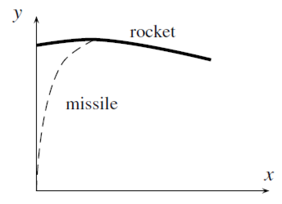
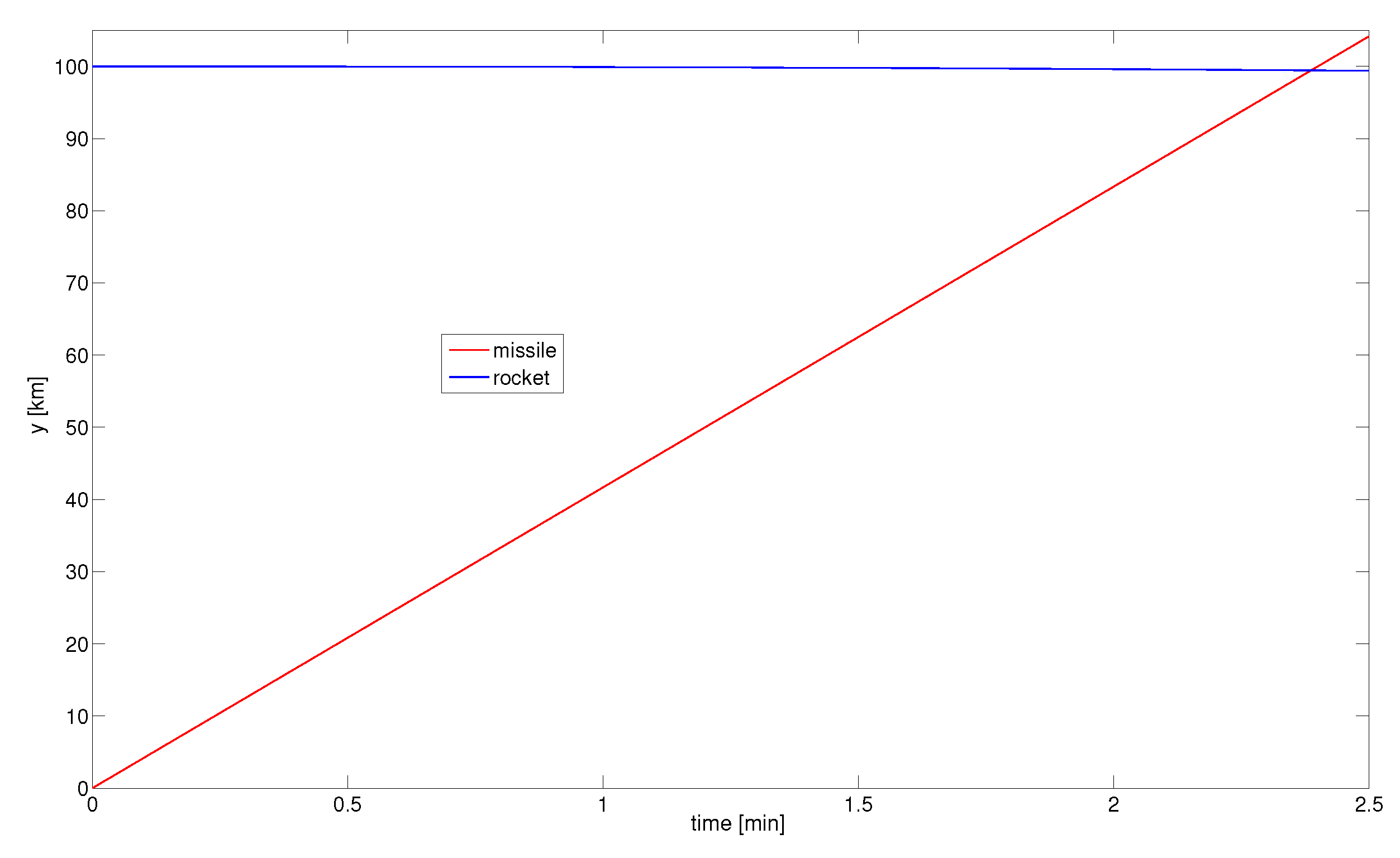
The interception process should take place when the ballistic rocket is in its descending phase of flight, whereas the missile continuously increases its altitude, as presented in Figure 3.

3. Performance Indices

In order to determine transversality conditions, and to mimic different behaviour of the system, three performance indices have been considered.

At all times, it is assumed that the optimal reference (input) w to the system is generated, to exert appropriate changes in x, y, to intercept a rocket. The performance indices presented below, refer to energy consumption or to the time-of-interception, which both have well-defined meanings.

3.1. Index $J_1$

The first performance index refers to minimization of energy of the input signals to the guidance system, since our control is open-loop based, and the problem is of generation of optimal input. In such a case,

$$\begin{array}{c}\hfill J_1={\int }_{t_0}^{t_f}\left(w_x^2\left(t\right)+s{w}_y^2\left(t\right)\right)dt,\end{array}$$

(14)

where s is the weight between the components. The input signal should satisfy dynamic equations of the rocket, and in both dimensions it should be the same, thus:

$$\begin{array}{ccc}\hfill w_x& =& \frac{T}{k}\dot{x}+\frac{1}{k}x,\hfill \end{array}$$

(15)

$$\begin{array}{ccc}\hfill w_y& =& \frac{T}{k}\dot{y}+\frac{1}{k}y,\hfill \end{array}$$

(16)

where $w_x$ denotes the position along the x axis, and $w_y$ along the y axis, T is a time constant, and k is the gain. The function under the integral takes the form:

$$\begin{array}{c}\hfill f(t,x,\dot{x},y,\dot{y})=\frac{T^2}{k^2}{\dot{x}}^2+\frac{2T}{k^2}\dot{x}x+\frac{1}{k^2}{x}^2+s\frac{T^2}{k^2}{\dot{y}}^2+s\frac{2T}{k^2}\dot{y}y+s\frac{1}{k^2}{y}^2.\end{array}$$

(17)

Euler equations derivatives:

$$\begin{array}{ccc}\hfill \frac{\partial f}{\partial x}& =& \frac{2T}{k^2}\dot{x}+\frac{2}{k^2}x,\hfill \end{array}$$

(18)

$$\begin{array}{ccc}\hfill \frac{\partial f}{\partial \dot{x}}& =& \frac{2T^2}{k^2}\dot{x}+\frac{2T}{k^2}x,\hfill \end{array}$$

(19)

$$\begin{array}{ccc}\hfill \frac{d}{dt}\left(\frac{\partial f}{\partial \dot{x}}\right)& =& \frac{2T^2}{k^2}\ddot{x}+\frac{2T}{k^2}\dot{x},\hfill \end{array}$$

(20)

giving the E–L equation

$$T^2\ddot{x}-x=0,$$

(21)

which solution becomes $x\left(t\right)=C_1{exp}^{-\frac{t}{T}}+C_2{exp}^{\frac{t}{T}}$.

By performing similar calculations in the y axis, one obtains $y\left(t\right)=C_3{exp}^{-\frac{t}{T}}+C_4{exp}^{\frac{t}{T}}$.

Since we have five unknowns ($C_1$, $C_2$, $C_3$, $C_4$, $t_f$) the following boundary conditions must be used:

$$\begin{array}{ccc}\hfill x\left(0\right)& =& 0,\hfill \end{array}$$

(22)

$$\begin{array}{ccc}\hfill x\left(t_k\right)& =& {\phi }_x\left(t_k\right),\hfill \end{array}$$

(23)

$$\begin{array}{ccc}\hfill y\left(0\right)& =& 0,\hfill \end{array}$$

(24)

$$\begin{array}{ccc}\hfill y\left(t_k\right)& =& {\phi }_y\left(t_k\right),\hfill \end{array}$$

(25)

$$\begin{array}{ccc}\hfill {\left.\left[(\dot{x}-{\dot{\varphi }}_x)\frac{\partial f}{\partial \dot{x}}\right]\right|}_{t=t_k}+{\left.\left[(\dot{y}-{\dot{\varphi }}_y)\frac{\partial f}{\partial \dot{y}}\right]\right|}_{t=t_k}& =& f\left(t_f\right).\hfill \end{array}$$

(26)

Finally, a single equation is obtained

$$\begin{array}{c}\hfill C_2^2-gT{C}_2{exp}^{\frac{t_f}{T}}+C_4^{2}s-2a{g}^{2}T{C}_{4}s{t}_f{exp}^{\frac{t_f}{T}}+2a{g}^{2}T{C}_{4}ps{exp}^{\frac{t_f}{T}}=0.\end{array}$$

(27)

3.2. Index $J_2$

In the second performance index, only energy along the y axis is considered, since along the x axis the trajectory moves according to the linear equation of motion $x=gt$, thus

$$\begin{array}{c}\hfill J_2={\int }_{t_0}^{t_f}{w}_y^2\left(t\right)dt,\end{array}$$

(28)

where

$$f(t,y,\dot{y})=\frac{T^2}{k^2}{\dot{y}}^2+\frac{2T}{k^2}\dot{y}y+\frac{1}{k^2}{y}^2.$$

(29)

By performing similar calculations as in the case of $J_1$ one obtains the E–L equation

$$\begin{array}{c}\hfill T^2\ddot{y}-y=0,\end{array}$$

(30)

and thus $y\left(t\right)=C_1{exp}^{-\frac{t}{T}}+C_2{exp}^{\frac{t}{T}}$.

The border conditions become:

$$\begin{array}{ccc}\hfill y\left(0\right)& =& 0,\hfill \end{array}$$

(31)

$$\begin{array}{ccc}\hfill y\left(t_f\right)& =& {\phi }_y\left(t_f\right),\hfill \end{array}$$

(32)

$$\begin{array}{ccc}\hfill {\left.\left[(\dot{y}-{\dot{\varphi }}_y)\frac{\partial f}{\partial \dot{y}}\right]\right|}_{t=t_f}& =& f\left(t_f\right).\hfill \end{array}$$

(33)

Finally, a single equation is obtained

$$\begin{array}{c}\hfill 2aT{t}_f\left({exp}^{\frac{2t_f}{T}}-1\right)+2aTp\left(1-{exp}^{\frac{2t_f}{T}}\right)=a{(t_f-p)}^2+q.\end{array}$$

(34)

3.3. Index $J_3$

This index is connected to minimum-time control that requires the velocity constraint $\dot{y}=v_{\max }$ to be introduced, otherwise the input command becomes infinite. The performance index is of the form

$$J_3={\int }_{t_0}^{t_f}dt.$$

(35)

There are no constraints imposed on the translation in x axis, since the movement in x axis is proportional to time (${\phi }_x\left(t\right)=gt$), thus minimum time implies minimal value of ${\phi }_x$. Taking this constraint into consideration, the performance index takes the form

$$J_3={\int }_{t_0}^{t_f}\left(1+\lambda (v_{\max }-\dot{y})\right)dt.$$

(36)

Euler equations derivatives for y:

$$\begin{array}{ccc}\hfill \frac{\partial f}{\partial y}& =& 0,\hfill \end{array}$$

(37)

$$\begin{array}{ccc}\hfill \frac{\partial f}{\partial \dot{y}}& =& -\lambda ,\hfill \end{array}$$

(38)

$$\begin{array}{ccc}\hfill \frac{d}{dt}\left(\frac{\partial f}{\partial \dot{y}}\right)& =& -\dot{\lambda },\hfill \end{array}$$

(39)

and for $\lambda$:

$$\begin{array}{ccc}\hfill \frac{\partial f}{\partial \lambda }& =& v_{\max }-\dot{y},\hfill \end{array}$$

(40)

$$\begin{array}{ccc}\hfill \frac{\partial f}{\partial \dot{\lambda }}& =& 0,\hfill \end{array}$$

(41)

$$\begin{array}{ccc}\hfill \frac{d}{dt}\left(\frac{\partial f}{\partial \dot{\lambda }}\right)& =& 0\hfill \end{array}$$

(42)

yield in the following set of E–L equations:

$$\begin{array}{ccc}\hfill \dot{\lambda }& =& 0,\hfill \end{array}$$

(43)

$$\begin{array}{ccc}\hfill \dot{y}& =& v_{\max },\hfill \end{array}$$

(44)

with the solutions:

$$\begin{array}{ccc}\hfill \lambda & =& C_1,\hfill \end{array}$$

(45)

$$\begin{array}{ccc}\hfill y& =& v_{\max }t+C_2.\hfill \end{array}$$

(46)

Border conditions become:

$$\begin{array}{ccc}\hfill y\left(0\right)& =& 0,\hfill \end{array}$$

(47)

$$\begin{array}{ccc}\hfill y\left(t_f\right)& =& {\phi }_y\left(t_f\right),\hfill \end{array}$$

(48)

and, as a result,

$$a{t}_f^2-(2ap+v_{\max })t_f+a{p}^2+q=0.$$

(49)

From the latter equation, one can obtain the interception time. In the x axis, it is assumed that the equation of motion becomes

$$x\left(t\right)=C_3{exp}^{-\frac{t}{T}}+C_4{exp}^{\frac{t}{T}}$$

(50)

with border conditions:

$$\begin{array}{ccc}\hfill x\left(0\right)& =& 0,\hfill \end{array}$$

(51)

$$\begin{array}{ccc}\hfill x\left(t_f\right)& =& g{t}_f,\hfill \end{array}$$

(52)

where $t_f$ is already calculated for y.

4. Implementation Issues, Results

4.1. Simulation Parameters

In all the considered interception problems, a single equation binding interception time has been obtained that needed to be solved, using numerical methods with sampling time $T_S=0.3\mathrm{s}$, resulting from observation of time constants of the obtained plots and on the basis of multiple simulations, and observations of performance indices behaviour.

The following parameters have been set as default values:

• $T=\frac{3.25}{60}\mathrm{h}$,
• $k=0.25$,
• $p=0.25\mathrm{h}$,
• $q=100\mathrm{km}$,
• $a=-10$,
• $g=400\mathrm{kmph}$,
• $h=40\mathrm{kmph}$,
• $v_{\max }=2500\mathrm{kmph}$,
• $s=0.00045\mathrm{h}$.

It is to be stressed that parameter s has been chosen in such a way so as to obtain interception time in minutes, to avoid false results.

4.2. Simulation Results

Below, the optimal curves for performance indices considered are included:

• index $J_1$ ($J_1^{*}=1401$):

  $$\begin{array}{ccc}\hfill x^{*}\left(t\right)& =& -8.4274{exp}^{-\frac{t}{3.25}}+8.4274{exp}^{\frac{t}{3.25}},\hfill \\ \hfill y^{*}\left(t\right)& =& -30.8138{exp}^{-\frac{t}{3.25}}+30.8138{exp}^{\frac{t}{3.25}},\hfill \\ \hfill w_x^{*}& =& 67.40{exp}^{\frac{t}{3.25}},\hfill \\ \hfill w_y^{*}& =& 246.50{exp}^{\frac{t}{3.25}},\hfill \\ \hfill t_f& =& 4.0889\min ;\hfill \end{array}$$
• index $J_2$ ($J_2^{*}=17,240$):

  $$\begin{array}{ccc}\hfill x^{*}\left(t\right)& =& 400t(\mathrm{known}\mathrm{in}\mathrm{advance}),\hfill \\ \hfill y^{*}\left(t\right)& =& -1.3513{exp}^{-\frac{t}{3.25}}+1.3513{exp}^{\frac{t}{3.25}},\hfill \\ \hfill w_y^{*}& =& 10.80{exp}^{\frac{t}{3.25}},\hfill \\ \hfill t_f& =& 13.9888\min ;\hfill \end{array}$$
• index $J_3$ ($J_3^{*}=0.039$):

  $$\begin{array}{ccc}\hfill x^{*}\left(t\right)& =& -9.9156{exp}^{-\frac{t}{3.25}}+9.9156{exp}^{\frac{t}{3.25}},\hfill \\ \hfill y^{*}\left(t\right)& =& 2500t,\hfill \\ \hfill w_x^{*}& =& 79.30{exp}^{\frac{t}{3.25}},\hfill \\ \hfill w_y^{*}& =& 1000t+542,\hfill \\ \hfill t_f& =& 2.3894\min ;\hfill \end{array}$$

In Figure 4, Figure 5 and Figure 6, the visualisation of the obtained results is presented in y axis, to show the interception takes place at the calculated time instants, whereas in Figure 7, Figure 8 and Figure 9, the reference inputs are shown, respectfully.

5. Software Program to Calculate Optimal Interception Time

The software program with the GUI in Matlab has been created that solves using Symbolic Toolbox the equations defining interception time instants $t_f$, calculates integration constants, and visualises the results.

Its main window is presented in Figure 10, where it is possible to define the task giving p, q, T, $V_{\max }$, choosing the appropriate performance index to minimize ($J_1$, $J_2$, $J_3$) and dimensionality of the problem (1D, 2D). After pressing Simulation button, the calculations are executed, with the final plot drawn at the end, see Figure 11.

Optionally, it is also possible to perform parametric analysis. where in different windows one can choose simulations for three different values of parameters from the list: p, q, T, $V_{\mathrm{x}}$, for which appropriate plots of x, y, $w_x$, $w_y$ are automatically drawn, with performance indices and interception time instants printed.

The software program will be made available in the open code, as m-files, in the MMD Database (see [19]), to enable further development of the program by interested researchers, and on the web page of Applied Control Techniques research group (http://act.put.poznan.pl). It can also be found at the link in the Supplementary section.

In order to make use of the derived equations and optimal trajectories, one can perform a sample parametric analysis. For example, Figure 12 presents results from 2D case with $T_x=1\min$, $T_y=2\min$, and $J_2$ index. In all the cases, $a=-10$, $k=0.25$, $g=400\mathrm{kmph}$, $s=0.45$.

6. Summary

The paper presents the application of variational calculus to the optimal interception task, and is accompanied by the software program enabling conducting multiple simulations and analyses. The program is easily modified, e.g., by including new performance indices, becoming a good simulation platform for possible research. In the due course of the research, a 3D task should be solved, accompanied by the problem of optimal launch time of the interception rocket from a mobile, e.g., train platform, launcher, utilising transversality conditions. The other direction of possible research would be to apply Pontryagin’s Minimum Principle to streamline the derivation phase of the formulas in the case of a more complicated model of the missile.

References

1. Yakimenko, O.A.; Lukacs, J.A. Trajectory-Shaping Guidance for Interception of Ballistic Missiles during the Boost Phase. J. Guid. Control. Dyn. 2008, 31, 1524–1531. [Google Scholar] [CrossRef]
2. Shinar, J.; Zarkh, M. Interception of Maneuvering tactical ballistic missiles in the atmoshphere. In ICAS Proceedings; American INST of Aeronautics and Astronautics: Reston, VA, USA, 1994; pp. 1354–1363. [Google Scholar]
3. Yournas, I.; Aqeel, A. A Genetic algorithm for mid-air target interception. Int. J. Comput. Appl. 2011, 14, 38–42. [Google Scholar]
4. Yeboles, D.M. Analysis and Optimization of Trajectories for Ballistic Missles Interception. Ph.D. Thesis, Universidad Politechnica de Madrid, Madrid, Spain, 2015. [Google Scholar]
5. Owczarkowski, A.; Horla, D.; Zietkiewicz, J. Introduction of Feedback Linearization to Robust LQR and LQI Control—Analysis of Results from an Unmanned Bicycle Robot with Reaction Wheel. Asian J. Control. 2019, 21, 1028–1040. [Google Scholar] [CrossRef]
6. Owczarkowski, A.; Horla, D. Robust LQR and LQI control with actuator failure of a 2DOF unmanned bicycle robot stabilized by an interial wheel. Int. J. Appl. Math. Comput. Sci. 2016, 26, 325–334. [Google Scholar] [CrossRef]
7. Zietkiewicz, J. Nonlinear Predictive Control with Constraint Propagation Strategy. In Proceedings of the 18th International Conference on Mechatronics, Brno, Czech Republic, 5–7 December 2018; pp. 222–228. [Google Scholar]
8. Giernacki, W.; Sadalla, T. Comparison of Tracking Performance and Robustness of Simplified Models of Multirotor UAV’s Propulsion Unit with CDM and PID Controllers. J. Control. Eng. Appl. Inform. 2017, 19, 31–40. [Google Scholar]
9. Na, H.; Lee, J.-I. Optimal Arrangement of Missile Defense Systems Considering Kill-Probability. In IEEE Transactions on Aerospace and Electronic Systems (Early Access); IEEE: Piscataway, NJ, USA, 2019. [Google Scholar]
10. Easthope, P.F. Probability of track impact in defended area: Use of Green’s theorem in the plane. Studia z Automatyki i Informatyki 2018, 43, 65–72. [Google Scholar]
11. Gelfand, I.; Fomin, S. Calculus of Variations; Prentice Hall: Upper Saddle River, NJ, USA, 1963. [Google Scholar]
12. Ballistic Missile. Available online: https://en.wikipedia.org/wiki/Ballistic_missile (accessed on 15 April 2019).
13. Pietrasienski, J.; Warchulski, M.; Warchulski, J. Simulation Research on TBM’s Shooting down by HIMAD SA-5 GAMMON AA system. Mechanik 2012, 85, 769–774. [Google Scholar]
14. Rocket and Space Technology. Basics of Space Flight: Rocket Propulsion. Available online: https://www.braeunig.us/space/propuls.htm (accessed on 20 March 2019).
15. Davis, D. Conservation of Momentum. Rocket Propulsion. Course 1351: General Physics I. Available online: https://www.ux1.eiu.edu/~cfadd/1350/09Mom/Rock.html (accessed on 20 April 2019).
16. HyperPhysics. Rocket Principles. Available online: http://hyperphysics.phy-astr.gsu.edu/hbase/rocket.html (accessed on 15 May 2019).
17. 9K720 Iskander. Available online: https://en.wikipedia.org/wiki/9K720_Iskander (accessed on 2 April 2019).
18. Mesko. The 120 mm Armor Piercing Fin Stabilized Discarding Sabot Tracer Target Practice (APFSDS-T-TP) for Rh 120 L44 Tank Gun. Available online: www.mesko.com.pl (accessed on 10 May 2019).
19. Giernacki, W.; Horla, D.; Sadalla, T. Mathematical models database (MMD ver. 1.0) non-commercial proposal for researchers. In Proceedings of the 21st International Conference on Methods and Models in Automation and Robotics, Miedzyzdroje, Poland, 29 August–1 September 2016; pp. 555–558. [Google Scholar]
Figure 1. Model of the rocket control system.
Algorithms 12 00148 g001
Figure 2. Observer position.
Algorithms 12 00148 g002
Figure 3. Interception process.
Algorithms 12 00148 g003
Figure 4. Solution minimizing J 1 .
Algorithms 12 00148 g004
Figure 5. Solution minimizing J 2 .
Algorithms 12 00148 g005
Figure 6. Solution minimizing J 3 .
Algorithms 12 00148 g006
Figure 7. Reference signal minimizing J 1 .
Algorithms 12 00148 g007
Figure 8. Reference signal minimizing J 2 .
Algorithms 12 00148 g008
Figure 9. Reference signal minimizing J 3 .
Algorithms 12 00148 g009
Figure 10. Main menu of the software program.
Algorithms 12 00148 g010
Figure 11. Visualisation of the interception process for default parameters.
Algorithms 12 00148 g011
Figure 12. Interception time t f as a function of p and q for minimized J 2 index (2D task).
Algorithms 12 00148 g012