An Optimized Differential Step-Size LMS Algorithm

Abstract

Adaptive algorithms with differential step-sizes (related to the filter coefficients) are well known in the literature, most frequently as “proportionate” algorithms. Usually, they are derived on a heuristic basis. In this paper, we introduce an algorithm resulting from an optimization criterion. Thereby, we obtain a benchmark algorithm and also another version with lower computational complexity, which is rigorously valid for less correlated input signals. Simulation results confirm the theory and outline the performance of the algorithms. Unfortunately, the good performance is obtained by an important increase in computational complexity. Nevertheless, the proposed algorithms could represent useful benchmarks in the field.

1. Introduction

System identification is a widespread application, where an adaptive filter is used to identify the impulse response of an unknown system [1]. Using the same input signal, the main idea is to determine the coefficients of this filter so that its output generates a signal which is as close as possible to the output signal of the unknown system that must be identified. In many applications, the impulse response of the unknown system is characterized by a small percentage of coefficients with high magnitude, while the rest of them are almost zero. Consequently, the adaptive filter can exploit this sparseness feature in order to improve its overall performance (especially in terms of convergence rate and tracking). The basic idea is to “proportionate” the algorithm behavior, i.e., to update each coefficient of the filter independently of the others, by adjusting the adaptation step-size in proportion to the magnitude of the estimated filter coefficient. In this manner, the adaptation gain is “proportionately” redistributed among all the coefficients, emphasizing the large ones (in magnitude) in order to speed up their convergence. In other words, larger coefficients receive larger step-sizes, thus increasing the convergence rate of those coefficients. This has the effect that active coefficients are adjusted faster than the non-active ones (i.e., small or zero coefficients). On the other hand, the proportionate algorithms could be sensitive to the sparseness degree of the system, i.e., the convergence rate could be reduced when the impulse responses are not very sparse.

A typical application of these algorithms is the echo cancellation problem, with emphasis on the identification of sparse echo paths. Among the most popular such algorithms are proportionate normalized least-mean-square (PNLMS) [2], PNLMS++ [3], and improved PNLMS (IPNLMS) [4] algorithms. Furthermore, many algorithms have been designed in order to exploit the sparseness character of the unknown system [5,6,7], while their main focus is to improve both the convergence rate and tracking ability [8,9,10]. However, most of these algorithms have been designed in a heuristic manner. For example, in the case of the celebrated PNLMS algorithm [2], the equations used to calculate the step-size control factors are not based on any optimization criteria but are designed in an ad hoc way. For this reason, after an initial fast convergence phase, the convergence rate of the PNLMS algorithm significantly slows down. Nevertheless, following the PNLMS idea, other more sophisticated algorithms working on the same principle have been proposed with the ultimate purpose to fully exploit sparsity of impulse responses. Among them, the IPNLMS algorithm [4] represents a benchmark solution, which is more robust to the sparseness degree of the impulse response.

A connection could be established between proportionate algorithms and variable step-size adaptive filters. In terms of their purpose, both categories adjust the step-size in order to enhance the overall performance. While proportionate filters aim to improve the convergence rate by increasing the adaptation step-size of the larger coefficients, variable step-size algorithms target the well-known compromise between the convergence rate and misadjustment [1]. In both cases, the adaptation control rules should rely on some specific optimization criteria.

Based on the initial work reported in [11,12], in this paper, we propose a least-mean-square (LMS) algorithm controlled by a diagonal matrix, $\mathbf{Y}$, instead of a usual scalar step-size. The elements of the matrix are adjusted at each iteration by considering the mean-squared deviation (MSD) minimization. Hence, following a stochastic model [13], we obtain an optimized differential step-size LMS (ODSS-LMS) algorithm, tailored by a state variable model. The theory has been driven on the model of an unknown system characterized by a time-varying behavior. The algorithm developed in [12], namely the optimized LMS algorithm with individual control factors (OLMS-ICF), represents only a particular case of the ODSS-LMS algorithm.

The motivation behind our approach can be summarized as follows. In many related works concerning optimized step-size algorithms, e.g., [14,15,16,17,18], the reference signal is considered the output of a time-invariant system corrupted by additive noise. However, in realistic scenarios, the system to be identified could be variable in time. For example, in acoustic echo cancellation, it can be assumed that the impulse response of the echo path is modeled by a time-varying system following a first-order Markov model [13]. In addition, it makes more sense to minimize the system misalignment (in terms of the MSD of the coefficients), instead of the classical error-based cost function. The reason is that, in real-world system identification problems, the goal of the adaptive filter is not to make the error signal goes to zero. The objective, instead, is to recover the additive noise (which corrupts the system’s output) from the error signal of the adaptive filter, after this one converges to the true solution. For example, in echo cancellation, this “corrupting noise” comes from the near-end and could also contain the voice of the near-end talker. Consequently, it should be delivered (with little or no distortion) to the far-end, through the error signal.

This paper is structured as follows. In Section 2, we describe the system model. Furthermore, the autocorrelation matrix of the coefficients error is introduced in Section 3. We develop the ODSS-LMS algorithm in Section 4, as well as a simplified version for a white Gaussian input. Simulations of the proposed algorithms are shown in Section 5. Finally, conclusions are discussed in Section 6.

2. System Model

We begin with the traditional steepest descent update equation [11]:

$$\begin{array}{cc}\hfill \widehat{\mathbf{w}}\left(n\right)& =\widehat{\mathbf{w}}(n-1)+\mu \mathrm{E}\left[\mathbf{x}\left(n\right)\alpha \left(n\right)\right].\hfill \end{array}$$

(1)

In Equation (1), we denote $\widehat{\mathbf{w}}\left(n\right)={\left[\begin{array}{cccc}{\widehat{w}}_0\left(n\right)& {\widehat{w}}_1\left(n\right)& \cdots & {\widehat{w}}_{L-1}\left(n\right)\end{array}\right]}^T$ as the adaptive filter (of length L), where the superscript ${}^T$ is the transpose operator, $\mu$ is the fixed step-size, $\mathbf{x}\left(n\right)={\left[\begin{array}{cccc}x\left(n\right)& x(n-1)& \cdots & x(n-L+1)\end{array}\right]}^T$ is a vector that contains the L most recent real-valued samples of the (zero-mean) input signal at the discrete time index n, $\alpha \left(n\right)$ is the a priori error signal, and $\mathrm{E}(·)$ is the statistical expectation. The goal of the adaptive filter is to estimate the impulse response of the unknown system denoted as $\mathbf{w}\left(n\right)={\left[\begin{array}{cccc}{w}_0\left(n\right)& w_1\left(n\right)& \cdots & w_{L-1}\left(n\right)\end{array}\right]}^T$. Using the previous notation, the a priori error is expressed as $\alpha \left(n\right)=d\left(n\right)-{\mathbf{x}}^T\left(n\right)\widehat{\mathbf{w}}(n-1)$, where the desired signal, $d\left(n\right)={\mathbf{x}}^T\left(n\right)\mathbf{w}\left(n\right)+v\left(n\right)$, consists of the output of the unknown system corrupted by the measurement noise, $v\left(n\right)$, which is assumed to be a zero-mean Gaussian noise signal.

Then, by applying the stochastic gradient principle and substituting the fixed step-size with a diagonal matrix, $\mathbf{Y}\left(n\right)$, the coefficients of the estimated impulse response can be updated as follows:

$$\begin{array}{cc}\hfill \widehat{\mathbf{w}}\left(n\right)& =\widehat{\mathbf{w}}(n-1)+\mathbf{Y}\left(n\right)\mathbf{x}\left(n\right)\alpha \left(n\right).\hfill \end{array}$$

(2)

Considering a stochastic system model described by $\mathbf{w}\left(n\right)=\mathbf{w}(n-1)+{\mathit{\delta }}_{\mathbf{w}}\left(n\right)$, where ${\mathit{\delta }}_{\mathbf{w}}\left(n\right)$ is a zero-mean Gaussian random vector, the goal consists of finding the diagonal matrix, $\mathbf{Y}\left(n\right)$, that minimizes at each iteration the MSD, $m\left(n\right)=\mathrm{E}\left[{\mathbf{c}}^T\left(n\right)\mathbf{c}\left(n\right)\right]$, where $\mathbf{c}\left(n\right)=\widehat{\mathbf{w}}\left(n\right)-\mathbf{w}\left(n\right)$ denotes the a posteriori misalignment. Thereby, the a posteriori error of the adaptive filter is

$$\begin{array}{cc}\hfill e\left(n\right)& =d\left(n\right)-{\mathbf{x}}^T\left(n\right)\widehat{\mathbf{w}}\left(n\right).\hfill \end{array}$$

(3)

Substituting the desired signal and the a posteriori misalignment in Equation (3), the a posteriori error becomes $e\left(n\right)=v\left(n\right)-{\mathbf{x}}^T\left(n\right)\mathbf{c}\left(n\right)$. Proceeding in the same manner with the a priori error, we obtain $\alpha \left(n\right)={\mathbf{x}}^T\left(n\right)\left[{\mathit{\delta }}_{\mathbf{w}}\left(n\right)-\mathbf{c}(n-1)\right]+v\left(n\right)$. Therefore, we can introduce (2) in the a posteriori misalignment to obtain the recursive relation:

$$\begin{array}{c}\hfill \mathbf{c}\left(n\right)=\mathbf{c}(n-1)+\mathbf{w}(n-1)-\mathbf{w}\left(n\right)+\mathbf{Y}\left(n\right)\mathbf{x}\left(n\right)\alpha \left(n\right).\end{array}$$

(4)

Furthermore, we can process Equation (4) as follows:

$$\begin{array}{cc}\mathbf{c}\left(n\right)\hfill & =\mathbf{c}(n-1)-{\mathit{\delta }}_{\mathbf{w}}\left(n\right)+\mathbf{Y}\left(n\right)\mathbf{x}\left(n\right)\alpha \left(n\right)\hfill \\ & =\mathbf{c}(n-1)-{\mathit{\delta }}_{\mathbf{w}}\left(n\right)+\mathbf{Y}\left(n\right)\mathbf{x}\left(n\right)\{{\mathbf{x}}^T\left(n\right)\left[{\mathit{\delta }}_{\mathbf{w}}\left(n\right)-\mathbf{c}(n-1)\right]+v\left(n\right)\}\hfill \\ & =[{\mathbf{I}}_L-\mathbf{Y}\left(n\right)\mathbf{x}\left(n\right){\mathbf{x}}^T\left(n\right)][\mathbf{c}(n-1)-{\mathit{\delta }}_{\mathbf{w}}\left(n\right)]+\mathbf{Y}\left(n\right)\mathbf{x}\left(n\right)v\left(n\right),\hfill \end{array}$$

(5)

where ${\mathbf{I}}_L$ is the identity matrix of size $L\times L$.

3. Autocorrelation Matrix of the Coefficients Error

In this framework, we assume that the input signal is wide-sense stationary. Therefore, its autocorrelation matrix is given by $\mathbf{R}=\mathrm{E}\left[\mathbf{x}\left(n\right){\mathbf{x}}^T\left(n\right)\right]$. The autocorrelation matrix of the coefficients error is

$$\begin{array}{cc}\hfill {\mathbf{R}}_{\mathbf{c}}\left(n\right)& \triangleq \mathrm{E}\left[\mathbf{c}\left(n\right){\mathbf{c}}^T\left(n\right)\right].\hfill \end{array}$$

(6)

In addition, we denote $\mathbf{\Gamma }\left(n\right)\triangleq {\mathbf{R}}_{\mathbf{c}}\left(n\right)+{\sigma }_w^2{\mathbf{I}}_L$ and $\gamma \left(n\right)\triangleq \mathrm{diag}[\mathbf{\Gamma }(n\left)\right]$, where ${\sigma }_w^2$ is the variance of the system noise and $\mathrm{diag}(·)$ defines a vector retaining only the main diagonal elements of $\mathbf{\Gamma }\left(n\right)$. Going forward, Equation (5) is developed by applying the ${\ell }_2$ norm and the statistical expectation, so that we can introduce the notation:

$$\begin{array}{c}\hfill m\left(n\right)=\mathrm{E}\left[{∥\mathbf{c}\left(n\right)∥}_2^2\right]=\mathrm{tr}\left[{\mathbf{R}}_{\mathbf{c}}\left(n\right)\right],\end{array}$$

(7)

where $\mathrm{tr}(·)$ denotes the trace of a square matrix. Substituting (5) into (6), the autocorrelation matrix of the coefficients error results in

$$\begin{array}{cc}{\mathbf{R}}_{\mathbf{c}}\left(n\right)\hfill & =\mathrm{E}\{[{\mathbf{I}}_L-\mathbf{Y}\left(n\right)\mathbf{x}\left(n\right){\mathbf{x}}^T\left(n\right)][\mathbf{c}(n-1)-{\mathit{\delta }}_{\mathbf{w}}\left(n\right)]\hfill \\ & \times [{\mathbf{c}}^T(n-1)-{\mathit{\delta }}_{\mathbf{w}}^T\left(n\right)][{\mathbf{I}}_L-\mathbf{x}\left(n\right){\mathbf{x}}^T\left(n\right)\mathbf{Y}\left(n\right)]\hfill \\ & +\mathbf{Y}\left(n\right)\mathbf{x}\left(n\right){\mathbf{x}}^T\left(n\right)\mathbf{Y}\left(n\right)v^2\left(n\right)\}.\hfill \end{array}$$

(8)

At this point, we consider that ${\mathit{\delta }}_{\mathbf{w}}\left(n\right)$ is uncorrelated with the a posteriori misalignment at the discrete time index $n-1$ and with the input signal at the discrete time index n. In addition, we assume that $\mathbf{c}(n-1)$ and $\mathbf{x}\left(n\right)$ are uncorrelated. The zero-mean measurement noise, $v\left(n\right)$, is independent of the input signal, $\mathbf{x}\left(n\right)$, and of the system noise, ${\mathit{\delta }}_{\mathbf{w}}\left(n\right)$. The variance of the additive noise is ${\sigma }_v^2=E\left[v^2\left(n\right)\right]$. With these assumptions, the statistical expectation of the product term in (8) can be written as

$$\begin{array}{c}\mathrm{E}\left\{[{\mathbf{I}}_L-\mathbf{Y}\left(n\right)\mathbf{x}\left(n\right){\mathbf{x}}^T\left(n\right)][\mathbf{c}(n-1)-{\mathit{\delta }}_{\mathbf{w}}\left(n\right)][{\mathbf{c}}^T(n-1)-{\mathit{\delta }}_{\mathbf{w}}^T\left(n\right)][{\mathbf{I}}_L-\mathbf{x}\left(n\right){\mathbf{x}}^T\left(n\right)\mathbf{Y}\left(n\right)]\right\}\hfill \\ ={\mathbf{R}}_{\mathbf{c}}(n-1)+{\mathbf{I}}_L{\sigma }_w^2-[{\mathbf{R}}_{\mathbf{c}}(n-1)+{\mathbf{I}}_L{\sigma }_w^2]\mathbf{R}\mathbf{Y}\left(n\right)-\mathbf{Y}\left(n\right)\mathbf{R}[{\mathbf{R}}_{\mathbf{c}}(n-1)+{\mathbf{I}}_L{\sigma }_w^2]+\mathbf{Y}\left(n\right)\mathbf{Q}\left(n\right)\mathbf{Y}\left(n\right),\hfill \end{array}$$

(9)

where

$$\begin{array}{cc}\mathbf{Q}\left(n\right)\hfill & \triangleq \mathrm{E}\left\{\left[\mathbf{x}\left(n\right){\mathbf{x}}^T\left(n\right)\right][\mathbf{c}(n-1)-{\mathit{\delta }}_{\mathbf{w}}\left(n\right)][{\mathbf{c}}^T(n-1)-{\mathit{\delta }}_{\mathbf{w}}^T\left(n\right)]\left[\mathbf{x}\left(n\right){\mathbf{x}}^T\left(n\right)\right]\right\}\hfill \\ & =\mathrm{E}\left[\mathbf{x}\left(n\right){\mathbf{x}}^T\left(n\right)\mathbf{p}\left(n\right){\mathbf{p}}^T\left(n\right)\mathbf{x}\left(n\right){\mathbf{x}}^T\left(n\right)\right]\hfill \\ & =\mathrm{E}\left\{{\left[{\mathbf{p}}^T\left(n\right)\mathbf{x}\left(n\right)\right]}^2\mathbf{x}\left(n\right){\mathbf{x}}^T\left(n\right)\right\}\hfill \\ & =\mathrm{E}\left[\sum _{i,j=0}^{L-1}{p}_i\left(n\right)p_j\left(n\right)x(n-i)x(n-j)\widehat{\mathbf{R}}\left(n\right)\right]\hfill \end{array}$$

(10)

and

$$\begin{array}{cc}\hfill \widehat{\mathbf{R}}\left(n\right)& =\mathbf{x}\left(n\right){\mathbf{x}}^T\left(n\right),\hfill \end{array}$$

(11)

$$\begin{array}{cc}\hfill \mathbf{p}\left(n\right)& ={\mathit{\delta }}_{\mathbf{w}}\left(n\right)-\mathbf{c}(n-1)={[p_0\left(n\right)p_1\left(n\right)\cdots p_{L-1}\left(n\right)]}^T.\hfill \end{array}$$

(12)

Including Equation (11) in (10), we can express the elements of the matrix $\mathbf{Q}\left(n\right)$ as

$$\begin{array}{cc}\hfill {\left[\mathbf{Q}\left(n\right)\right]}_{r,l}& =\sum _{i,j=0}^{L-1}\mathrm{E}\left[p_i\left(n\right)p_j\left(n\right)\right]\mathrm{E}\left[x(n-i)x(n-j)x(n-r)x(n-l)\right],\hfill \end{array}$$

(13)

for $r,l=0,1,\dots ,L-1$. By applying the Gaussian moment factoring theorem [19], three terms can be defined as

$$\begin{array}{cc}{\left[{\mathbf{Q}}_1\left(n\right)\right]}_{r,l}\hfill & =\sum _{i,j=0}^{L-1}\mathrm{E}\left[p_i\left(n\right)p_j\left(n\right)\right]x(i-j)x(r-l)\hfill \\ & =x(r-l)\sum _{i,j=0}^{L-1}{[\mathbf{\Gamma }(n-1)]}_{i,j}x(i-j)\hfill \\ & =\mathrm{tr}[\mathbf{\Gamma }(n-1)\mathbf{R}]{\left[\mathbf{R}\right]}_{r,l},\hfill \end{array}$$

(14)

$$\begin{array}{cc}{\left[{\mathbf{Q}}_2\left(n\right)\right]}_{r,l}\hfill & =\sum _{i,j=0}^{L-1}\mathrm{E}\left[p_i\left(n\right)p_j\left(n\right)\right]x(i-r)x(j-l)\hfill \\ & =\sum _{i=0}^{L-1}{\mathbf{R}}_{r,i}\sum _{j=0}^{L-1}{[\mathbf{\Gamma }(n-1)]}_{i,j}{\mathbf{R}}_{j,l}\hfill \\ & ={[\mathbf{R}\mathbf{\Gamma }(n-1)\mathbf{R}]}_{r,l},\hfill \end{array}$$

(15)

and

$$\begin{array}{cc}{\left[{\mathbf{Q}}_3\left(n\right)\right]}_{r,l}\hfill & =\sum _{i,j=0}^{L-1}\mathrm{E}\left[p_i\left(n\right)p_j\left(n\right)\right]x(i-l)x(j-r)\hfill \\ & ={\left[{\mathbf{Q}}_2\left(n\right)\right]}_{r,l},\hfill \end{array}$$

(16)

with

$$\begin{array}{cc}\mathbf{Q}\left(n\right)\hfill & ={\mathbf{Q}}_1\left(n\right)+{\mathbf{Q}}_2\left(n\right)+{\mathbf{Q}}_3\left(n\right)\hfill \\ & =2\mathbf{R}\mathbf{\Gamma }(n-1)\mathbf{R}+\mathbf{R}\mathrm{tr}[\mathbf{\Gamma }(n-1\left)\mathbf{R}\right].\hfill \end{array}$$

(17)

Finally, the statistical expectation of the last term in Equation (8) is

$$\begin{array}{c}\hfill E\left[\mathbf{Y}\left(n\right)\mathbf{x}\left(n\right){\mathbf{x}}^T\left(n\right)\mathbf{Y}\left(n\right)v^2\left(n\right)\right]=\mathbf{Y}\left(n\right)\mathbf{R}\mathbf{Y}\left(n\right){\sigma }_v^2.\end{array}$$

(18)

Thus, we can summarize the autocorrelation matrix of the coefficients error as

$$\begin{array}{cc}{\mathbf{R}}_{\mathbf{c}}\left(n\right)\hfill & =\mathbf{\Gamma }(n-1)-\mathbf{\Gamma }(n-1)\mathbf{R}\mathbf{Y}\left(n\right)-\mathbf{Y}\left(n\right)\mathbf{R}\mathbf{\Gamma }(n-1)\hfill \\ & +\mathbf{Y}\left(n\right)\{2\mathbf{R}\mathbf{\Gamma }(n-1)\mathbf{R}+\mathbf{R}\mathrm{tr}[\mathbf{\Gamma }(n-1)\mathbf{R}\left]\right\}\mathbf{Y}\left(n\right)\hfill \\ & +\mathbf{Y}\left(n\right)\mathbf{R}\mathbf{Y}\left(n\right){\sigma }_v^2.\hfill \end{array}$$

(19)

4. ODSS-LMS Algorithm

Let us define $\mathbf{Y}\left(n\right)=\mathrm{mdiag}\left[\mathbf{y}\right(n\left)\right]$, where $\mathrm{mdiag}(·)$ denotes a diagonal matrix, having on its main diagonal the elements of the vector $\mathbf{y}\left(n\right)$. If the input argument is a matrix $\mathbf{A}$, then $\mathbf{B}=\mathrm{mdiag}\left(\mathbf{A}\right)$ returns a diagonal matrix $\mathbf{B}$, retaining only the elements of the main diagonal of $\mathbf{A}$.

4.1. Minimum MSD Value

Replacing $\mathbf{\Gamma }(n-1)$ and using (19), the MSD can be rewritten as

$$\begin{array}{cc}m\left(n\right)\hfill & =\mathrm{tr}\left\{[{\mathbf{R}}_{\mathbf{c}}(n-1)+{\sigma }_w^2{\mathbf{I}}_L]\{{\mathbf{I}}_L-\mathbf{R}\mathbf{Y}\left(n\right)-\mathbf{Y}\left(n\right)\mathbf{R}+{\sigma }_x^2\mathbf{R}\mathrm{tr}\left[{\mathbf{Y}}^2\left(n\right)\right]+2\mathbf{R}{\mathbf{Y}}^2\left(n\right)\mathbf{R}\}\right\}\hfill \\ & +\mathrm{tr}\left[{\sigma }_v^2\mathbf{R}{\mathbf{Y}}^T\left(n\right)\mathbf{Y}\left(n\right)\right],\hfill \end{array}$$

(20)

where ${\sigma }_x^2$ is the variance of the input signal, $x\left(n\right)$. The last term in (20) can be easily computed as

$$\begin{array}{c}\hfill \mathrm{tr}\left[{\sigma }_v^2\mathbf{R}{\mathbf{Y}}^T\left(n\right)\mathbf{Y}\left(n\right)\right]={\sigma }_x^2{\sigma }_v^2{\mathbf{y}}^T\left(n\right)\mathbf{y}\left(n\right).\end{array}$$

(21)

Therefore, the product term of (20) results in

$$\begin{array}{cc}\hfill & \mathrm{tr}\left\{{\mathbf{R}}_{\mathbf{c}}(n-1)\{{\mathbf{I}}_L-\mathbf{R}\mathbf{Y}\left(n\right)-\mathbf{Y}\left(n\right)\mathbf{R}+{\sigma }_x^2\mathbf{R}\mathrm{tr}\left[{\mathbf{Y}}^2\left(n\right)\right]+2\mathbf{R}{\mathbf{Y}}^2\left(n\right)\mathbf{R}\}\right\}\hfill \\ & =m(n-1)-2{\mathbf{y}}^T\left(n\right)\mathrm{diag}\left[\mathbf{R}{\mathbf{R}}_{\mathbf{c}}(n-1)\right]+{\sigma }_x^2\mathrm{tr}\left[{\mathbf{R}}_{\mathbf{c}}(n-1)\mathbf{R}\right]{\mathbf{y}}^T\left(n\right)\mathbf{y}\left(n\right)\hfill \\ & +2{\mathbf{y}}^T\left(n\right)\mathrm{mdiag}\left[\mathbf{R}{\mathbf{R}}_{\mathbf{c}}(n-1)\mathbf{R}\right]\mathbf{y}\left(n\right)\hfill \end{array}$$

(22)

and

$$\begin{array}{cc}\hfill & \mathrm{tr}\left\{{\sigma }_w^2\{{\mathbf{I}}_L-\mathbf{R}\mathbf{Y}\left(n\right)-\mathbf{Y}\left(n\right)\mathbf{R}+{\sigma }_x^2\mathbf{R}\mathrm{tr}\left[{\mathbf{Y}}^2\left(n\right)\right]+2\mathbf{R}{\mathbf{Y}}^2\left(n\right)\mathbf{R}\}\right\}\hfill \\ & ={\sigma }_w^2\{L-2{\mathbf{y}}^T\left(n\right)\mathbf{r}+L{\sigma }_x^4{\mathbf{y}}^T\left(n\right)\mathbf{y}\left(n\right)+2{\mathbf{y}}^T\left(n\right)\mathrm{mdiag}\left[{\mathbf{R}}^2\right]\mathbf{y}\left(n\right)\},\hfill \end{array}$$

(23)

with $\mathbf{r}\triangleq \mathrm{diag}\left(\mathbf{R}\right)$. Based on (20), (21), and (23), the MSD becomes

$$\begin{array}{cc}m\left(n\right)\hfill & =m(n-1)-2{\mathbf{y}}^T\left(n\right)\mathrm{diag}\left[\mathbf{R}{\mathbf{R}}_{\mathbf{c}}(n-1)\right]+{\sigma }_x^2\mathrm{tr}\left[{\mathbf{R}}_{\mathbf{c}}(n-1)\mathbf{R}\right]{\mathbf{y}}^T\left(n\right)\mathbf{y}\left(n\right)\hfill \\ & +2{\mathbf{y}}^T\left(n\right)\mathrm{mdiag}\left[\mathbf{R}{\mathbf{R}}_{\mathbf{c}}(n-1)\mathbf{R}\right]\mathbf{y}\left(n\right)\hfill \\ & +{\sigma }_w^2\{L-2{\mathbf{y}}^T\left(n\right)\mathbf{r}+L{\sigma }_x^4{\mathbf{y}}^T\left(n\right)\mathbf{y}\left(n\right)+2{\mathbf{y}}^T\left(n\right)\mathrm{mdiag}\left[{\mathbf{R}}^2\right]\mathbf{y}\left(n\right)\}\hfill \\ & +{\sigma }_x^2{\sigma }_v^2{\mathbf{y}}^T\left(n\right)\mathbf{y}\left(n\right).\hfill \end{array}$$

(24)

4.2. Optimum Step-Size Derivation

Taking the gradient of MSD with respect to $\mathbf{y}\left(n\right)$, it results in

$$\begin{array}{cc}{\nabla }_{\mathbf{y}\left(n\right)}\left[m\left(n\right)\right]\hfill & =-2\mathrm{diag}\left[\mathbf{R}{\mathbf{R}}_{\mathbf{c}}(n-1)\right]+2{\sigma }_x^2\mathrm{tr}\left[{\mathbf{R}}_{\mathbf{c}}(n-1)\mathbf{R}\right]\mathbf{y}\left(n\right)+4\mathrm{mdiag}\left[\mathbf{R}{\mathbf{R}}_{\mathbf{c}}(n-1)\mathbf{R}\right]\mathbf{y}\left(n\right)\hfill \\ & +{\sigma }_w^2[-2\mathbf{r}+2L{\sigma }_x^4\mathbf{y}\left(n\right)+4\mathrm{mdiag}\left({\mathbf{R}}^2\right)\mathbf{y}]+2{\sigma }_x^2{\sigma }_v^2\mathbf{y}\left(n\right).\hfill \end{array}$$

(25)

Solving the quadratic form of (25), we obtain the general optimal solution:

$$\begin{array}{c}\hfill {\mathbf{y}}_{\mathrm{o}}\left(n\right)={\left\{{\sigma }_x^2{\mathbf{I}}_L\{\mathrm{tr}[\mathbf{\Gamma }(n-1)\mathbf{R}]+{\sigma }_v^2\}+2\mathrm{mdiag}[\mathbf{R}\mathbf{\Gamma }(n-1)\mathbf{R}]\right\}}^{-1}\mathrm{diag}[\mathbf{R}\mathbf{\Gamma }(n-1)].\end{array}$$

(26)

In brief, (19), (24), and (26) represent the main equations of the optimized differential least-mean-square “general” (ODSS-LMS-G) algorithm.

4.3. Simplified Version

At this stage, we can define the main equations for the optimized differential least-mean-square “white” (ODSS-LMS-W) algorithm, in the scenario of a white Gaussian noise signal as input. This algorithm is similar to the OLMS-ICF algorithm presented in [12], which was developed based on the same simplified assumption.

Considering that $\mathbf{R}={\sigma }_x^2{\mathbf{I}}_L$, we can rewrite (19), (24), and (26) as

$$\begin{array}{cc}{\mathbf{R}}_{\mathbf{c}}\left(n\right)\hfill & =\mathbf{\Gamma }(n-1)-{\sigma }_x^2\mathbf{\Gamma }(n-1)\mathbf{Y}\left(n\right)-{\sigma }_x^2\mathbf{Y}\left(n\right)\mathbf{\Gamma }(n-1)\hfill \\ & +{\sigma }_x^4\mathbf{Y}\left(n\right)\{2\mathbf{\Gamma }(n-1)+{\mathbf{I}}_L\mathrm{tr}[\mathbf{\Gamma }(n-1)]\}\mathbf{Y}\left(n\right)+{\sigma }_x^2{\sigma }_v^2{\mathbf{Y}}^2\left(n\right),\hfill \end{array}$$

(27)

$$\begin{array}{cc}m\left(n\right)\hfill & =[m(n-1)+L{\sigma }_w^2][1+{\sigma }_x^4{\mathbf{y}}^T\left(n\right)\mathbf{y}\left(n\right)]-2{\sigma }_x^2{\gamma }^T(n-1)\mathbf{y}\left(n\right)\hfill \\ & +2{\sigma }_x^4{\mathbf{y}}^T\left(n\right)\mathrm{mdiag}\left[\gamma (n-1)\right]\mathbf{y}\left(n\right)+{\sigma }_v^2{\sigma }_x^2{\mathbf{y}}^T\left(n\right)\mathbf{y}\left(n\right),\hfill \end{array}$$

(28)

and

$$\begin{array}{c}\hfill {\mathbf{y}}_{\mathrm{o}}\left(n\right)={\left\{{\sigma }_x^2{\mathbf{I}}_L[m(n-1)+{\sigma }_w^2(L+2)]+2{\sigma }_x^2\mathrm{mdiag}\left[{\mathbf{R}}_{\mathbf{c}}(n-1)\right]+{\sigma }_v^2{\mathbf{I}}_L\right\}}^{-1}\gamma (n-1).\end{array}$$

(29)

Based on (27), we can define the recursive equation of $\gamma \left(n\right)$ as

$$\begin{array}{cc}\gamma \left(n\right)\hfill & =\gamma (n-1)+{\sigma }_w^2{\mathbf{1}}_{L\times 1}+2{\sigma }_x^2[{\sigma }_x^2{\mathbf{y}}_{\mathrm{o}}\left(n\right)-{\mathbf{1}}_{L\times 1}]\odot \gamma (n-1)\odot {\mathbf{y}}_{\mathrm{o}}\left(n\right)\hfill \\ & +{\sigma }_x^2\{{\sigma }_x^2\mathrm{tr}[\mathbf{\Gamma }(n-1)]+{\sigma }_v^2\}{\mathbf{y}}_{\mathrm{o}}\left(n\right)\odot {\mathbf{y}}_{\mathrm{o}}\left(n\right),\hfill \end{array}$$

(30)

where ${\mathbf{1}}_{L\times 1}$ denotes a vector with all its elements equal to one and ⊙ represents the Hadamard product. In order to verify the stability condition, let us define

$$\begin{array}{c}\hfill \mathbf{M}\left(n\right)\triangleq {\sigma }_x^2{\mathbf{I}}_L[m(n-1)+{\sigma }_w^2(L+2)]+2{\sigma }_x^2\mathrm{mdiag}\left[{\mathbf{R}}_{\mathbf{c}}(n-1)\right]+{\sigma }_v^2{\mathbf{I}}_L,\end{array}$$

(31)

which leads to ${\mathbf{y}}_{\mathrm{o}}\left(n\right)={\mathbf{M}}^{-1}\left(n\right)\gamma (n-1)$.

If the system is assumed to be time-invariant, i.e., ${\sigma }_w^2=0$, then

$$\begin{array}{cc}m\left(n\right)\hfill & =m(n-1)+{\mathbf{y}}^T\left(n\right)[{\sigma }_x^{4}m(n-1){\mathbf{I}}_L+2{\sigma }_x^4{\mathbf{R}}_{\mathbf{c}}(n-1)+{\mathbf{I}}_L{\sigma }_x^2{\sigma }_v^2]\mathbf{y}\left(n\right)-2{\sigma }_x^2{\gamma }^T(n-1)\mathbf{y}\left(n\right)\hfill \\ & =m(n-1)+{\sigma }_x^2{\mathbf{y}}^T\left(n\right)\mathbf{M}\left(n\right)\mathbf{y}\left(n\right)-2{\sigma }_x^2{\gamma }^T(n-1)\mathbf{y}\left(n\right)\hfill \\ & =m(n-1)-{\sigma }_x^2{\gamma }^T(n-1){\mathbf{M}}^{-1}\left(n\right)\gamma (n-1).\hfill \end{array}$$

(32)

Since $\mathbf{M}\left(n\right)$ is a diagonal positive definite matrix, $m\left(n\right)<m(n-1)$, therefore,

$$\begin{array}{cc}\hfill m\left(n\right)& =\sum _{l=0}^{L-1}{\gamma }_l(n-1)[1-{\sigma }_x^2{\mu }_l(n-1){\gamma }_l(n-1)],\hfill \end{array}$$

(33)

where ${\gamma }_l\left(n\right)$ denotes the lth element of the vector $\gamma \left(n\right)$ and

$$\begin{array}{c}\hfill {\mu }_l(n-1)\triangleq \frac{1}{m(n-1){\sigma }_x^2+2{\sigma }_x^2{\gamma }_l(n-1)+{\sigma }_v^2}.\end{array}$$

(34)

Based on (33) and (34), we can outline that

$$\begin{array}{c}\hfill \frac{{\sigma }_x^2{\gamma }_l(n-1)}{2{\sigma }_x^2{\gamma }_l(n-1)+{\sigma }_v^2+{\sigma }_x^2{\sum }_{i=0}^{L-1}{\gamma }_i(n-1)}<1,\end{array}$$

(35)

which guarantees the convergence. At the same time, the stability condition is verified, i.e., $0<m\left(n\right)<m(n-1)$.

4.4. Practical Considerations

The ODSS-LMS-G and ODSS-LMS-W algorithms are depicted in Algorithms 1 and 2, respectively. From a practical point of view, the variance ${\sigma }_x^2$ of the input signal could be estimated with a 1-pole exponential filter, or using ${\sigma }_x^2=(1/L){\mathbf{x}}^T\left(n\right)\mathbf{x}\left(n\right)$. In practice, the autocorrelation matrix of the input signal is not known and it can be estimated with a weighting window as ${\mathbf{R}}_{\mathbf{x}}\left(n\right)=\lambda {\mathbf{R}}_{\mathbf{x}}(n-1)+(1-\lambda )\mathbf{x}\left(n\right){\mathbf{x}}^T\left(n\right)$, where $\lambda =1-1/\left(PL\right)$, with $P>1$. The noise power ${\sigma }_v^2$ could be estimated in different ways as in [20,21]. The influence of the system noise variance ${\sigma }_w^2$ is analyzed in Section 5. Moreover, in order to obtain accurate estimates for some parameters, we suggest using an initialization algorithm such as the normalized LMS (NLMS) [11]. With the purpose to estimate the matrix ${\mathbf{R}}_{\mathbf{c}}\left(n\right)$ in the initial stage of the algorithm, we suppose that $\mathbf{c}\left(n\right)\approx \widehat{\mathbf{w}}\left(n\right)-\widehat{\mathbf{w}}(n-1)$, so that we can approximate it with the update term $\mathbf{u}\left(n\right)$ defined in Algorithms 1 and 2.

In terms of computational complexity, the matrix operations lead to a high computational complexity. Therewith, the matrix inversion operation is involved and contributes to the complexity increase. Taking into account once the terms that appear several times in multiple equations (i.e., $\mathbf{\Gamma }(n-1){\mathbf{R}}_{\mathbf{x}}\left(n\right)$, ${\mathbf{R}}_{\mathbf{x}}\left(n\right)\mathbf{\Gamma }(n-1)$), the computational complexity is summarized as follows. For the ODSS-LMS-G algorithm, the computation of the $\mathbf{M}\left(n\right)$ matrix requires $2L^3+2L+1$ multiplications and $2L^3-2L^2+2L$ additions, while its inversion consists of L divisions of the form $1/x$. Then, computation of the differential step-size ${\mathbf{y}}_{\mathrm{o}}\left(n\right)$ consists of $L^3+L$ multiplications and $L^3-L^2$ additions. The update term $\mathbf{u}\left(n\right)$ contributes with $2L$ multiplications. Thereto, because the $\mathbf{Y}\left(n\right)$ matrix is diagonal, the computation of the ${\mathbf{R}}_{\mathbf{c}}\left(n\right)$ matrix requires $8L$ multiplications and $5L$ additions. In addition, the computation of $\mathbf{\Gamma }\left(n\right)$ matrix requires L additions and the estimation of the ${\mathbf{R}}_{\mathbf{x}}\left(n\right)$ matrix imposes $2L^2+2L-1$ multiplications and $L^2$ additions. In case of the ODSS-LMS-W algorithm, several matrix operations disappear and the computational complexity decreases. Thus, the computation of the $\mathbf{M}\left(n\right)$ matrix requires only $2L+1$ multiplications and $2L+1$ additions. While $\mathbf{M}\left(n\right)$ matrix is diagonal, the computational complexity of its inversion involves L divisions. Therefore, the differential step-size ${\mathbf{y}}_{\mathrm{o}}\left(n\right)$ requires only L multiplications. In addition, the computation of the vector $\gamma \left(n\right)$ contributes with $5L+2$ multiplications and $5L$ additions. Furthermore, the MSD is obtained for L additions, while the update term $\mathbf{u}\left(n\right)$ adds $2L$ multiplications. Some equations are required in both algorithms. The coefficients update equation requires L additions and the a priori error computations consist of L multiplications and L additions. Last but not least, the initialization process of both algorithms involves $3L^2+2L+2$ multiplications, $L^2+L+3$ additions, and one division. In brief, without the complexity of the initialization process, the ODSS-LMS-G algorithm involves $3L^3+2L^2+16L$ multiplications, $3L^3-2L^2+9L$ additions, and L divisions, while ODSS-LMS-W consists of $10L+3$ multiplications, $10L+1$ additions, and L divisions. Note that the computational complexity analysis is based on the standard way of inverting and multiplying matrices, so that the computational complexity of the ODSS-LMS-G algorithm is $O\left(L^3\right)$. One of the first approaches regarding the reduction of matrix multiplication computational complexity is the Strassen algorithm [22], which is slightly better than the standard matrix multiplication algorithm, with a computational complexity of $O\left(L^{2.807}\right)$. Going forward, the Coppersmith–Winograd algorithm [23] could be used to reduce the matrix multiplication computational complexity to $O\left(L^{2.375}\right)$.

Algorithm 1: ODSS-LMS-G algorithm.

Initialization:

• $\widehat{\mathbf{w}}\left(0\right)={\mathbf{0}}_{L\times 1}$

• ${\mathbf{R}}_{\mathbf{c}}\left(0\right)=c{\mathbf{I}}_L$, where c is a small positive constant

• ${\mathbf{R}}_{\mathbf{x}}\left(0\right)={\mathbf{0}}_{L\times L}$

• $\mathbf{\Gamma }\left(0\right)={\mathbf{R}}_{\mathbf{c}}\left(0\right)+{\sigma }_w^2{\mathbf{I}}_L$

Parameters ${\sigma }_x^2,{\sigma }_v^2,{\sigma }_w^2$, known or estimated

$\lambda =1-\frac{1}{PL}$, with $P\ge 1$

For time index $n=1,2,\dots$:

• $\alpha \left(n\right)=d\left(n\right)-{\mathbf{x}}^T\left(n\right)\widehat{\mathbf{w}}(n-1)$

• ${\mathbf{R}}_{\mathbf{x}}\left(n\right)=\lambda {\mathbf{R}}_{\mathbf{x}}(n-1)+(1-\lambda )\mathbf{x}\left(n\right){\mathbf{x}}^T\left(n\right)$

If time index $n<KL$, with $K\ge 1$:

• $\mu \left(n\right)=\frac{\mu }{{\mathbf{x}}^T\left(n\right)\mathbf{x}\left(n\right)+\delta }$ (i.e., step-size of the NLMS algorithm)

• $\mathbf{u}\left(n\right)=\mu \left(n\right)\mathbf{x}\left(n\right)\alpha \left(n\right)$

• ${\mathbf{R}}_{\mathbf{c}}\left(n\right)=\lambda {\mathbf{R}}_{\mathbf{c}}(n-1)+(1-\lambda )\mathbf{u}\left(n\right){\mathbf{u}}^T\left(n\right)$

else:

• $\begin{array}{ll}\mathbf{M}\left(n\right)=\hfill & {\sigma }_x^2{\mathbf{I}}_L\{\mathrm{tr}[\mathbf{\Gamma }(n-1){\mathbf{R}}_{\mathbf{x}}\left(n\right)]+{\sigma }_v^2\}\hfill \\ & +2\mathrm{mdiag}[{\mathbf{R}}_{\mathbf{x}}\left(n\right)\mathbf{\Gamma }(n-1){\mathbf{R}}_{\mathbf{x}}\left(n\right)]\hfill \end{array}$

• ${\mathbf{y}}_{\mathrm{o}}\left(n\right)={\mathbf{M}}^{-1}\left(n\right)\mathrm{diag}[{\mathbf{R}}_{\mathbf{x}}\left(n\right)\mathbf{\Gamma }(n-1)]$

• $\mathbf{u}\left(n\right)={\mathbf{y}}_{\mathrm{o}}\left(n\right)\odot \mathbf{x}\left(n\right)\alpha \left(n\right)$

• $\mathbf{Y}\left(n\right)=\mathrm{mdiag}\left[{\mathbf{y}}_{\mathrm{o}}\left(n\right)\right]$

• $\begin{array}{ll}{\mathbf{R}}_{\mathbf{c}}\left(n\right)\hfill & =\mathbf{\Gamma }(n-1)-\mathbf{\Gamma }(n-1){\mathbf{R}}_{\mathbf{x}}\left(n\right)\mathbf{Y}\left(n\right)\hfill \\ & -\mathbf{Y}\left(n\right){\mathbf{R}}_{\mathbf{x}}\left(n\right)\mathbf{\Gamma }(n-1)+\mathbf{Y}\left(n\right)\{2{\mathbf{R}}_{\mathbf{x}}\left(n\right)\mathbf{\Gamma }(n-1){\mathbf{R}}_{\mathbf{x}}\left(n\right)\hfill \\ & +{\mathbf{R}}_{\mathbf{x}}\left(n\right)\mathrm{tr}[\mathbf{\Gamma }(n-1){\mathbf{R}}_{\mathbf{x}}\left(n\right)]\}\mathbf{Y}\left(n\right)+\mathbf{Y}\left(n\right){\mathbf{R}}_{\mathbf{x}}\left(n\right)\mathbf{Y}\left(n\right){\sigma }_v^2\hfill \end{array}$

• $\widehat{\mathbf{w}}\left(n\right)=\widehat{\mathbf{w}}(n-1)+\mathbf{u}\left(n\right)$

• $\mathbf{\Gamma }\left(n\right)={\mathbf{R}}_{\mathbf{c}}\left(n\right)+{\sigma }_w^2{\mathbf{I}}_L$

Finally, the overall computational complexity of the NLMS [1], IPNLMS [4], and JO-NLMS [24] algorithms is summarized for comparison. The NLMS algorithm consists of $2L+2$ multiplications, $2L+3$ additions, and 1 division, while the IPNLMS algorithm involves $5L+2$ multiplications, $5L$ additions, and two divisions. The JO-NLMS algorithm has a computational complexity similar to that of the NLMS algorithm, which is based on $2L+3$ multiplications, $2L+4$ additions, and one division. Notice that the computational complexity of these algorithms has been reported by considering ${\sigma }_x^2$, ${\sigma }_v^2$, and ${\sigma }_w^2$ parameters known, while their estimation depends on the implementation (e.g., in literature, different estimation methods are available). Of course, these algorithms do not involve matrix operations and the computational complexity is $O\left(L\right)$. At this point, it can be highlighted that the computational complexity of the ODSS-LMS-W algorithm is comparable with the complexity of the NLMS, IPNLMS, or JO-NLMS algorithm.

Even if the proposed algorithms present a high computational complexity, they are more affined to “benchmark” type algorithms and their performance is outlined in Section 5.

Algorithm 2: ODSS-LMS-W algorithm.

Initialization:    • $\widehat{\mathbf{w}}\left(0\right)={\mathbf{0}}_{L\times 1}$     • $m\left(0\right)=ϵ>0$     • $\gamma \left(0\right)=c{\mathbf{1}}_{L\times 1}$, where c is a small positive constant    • ${\mathbf{R}}_{\mathbf{c}}\left(0\right)=c{\mathbf{I}}_L$     • $\mathbf{\Gamma }\left(0\right)={\mathbf{R}}_{\mathbf{c}}\left(0\right)+{\sigma }_w^2{\mathbf{I}}_L$     Parameters ${\sigma }_x^2,{\sigma }_v^2,{\sigma }_w^2$, known or estimated     $\lambda =1-\frac{1}{PL}$, with $P\ge 1$          For time index $n=1,2,\dots$:    • $\alpha \left(n\right)=d\left(n\right)-{\mathbf{x}}^T\left(n\right)\widehat{\mathbf{w}}(n-1)$           If time index $n<KL$, with $K\ge 1$:        • $\mu \left(n\right)=\frac{\mu }{{\mathbf{x}}^T\left(n\right)\mathbf{x}\left(n\right)+\delta }$ (i.e., step-size of the NLMS algorithm)        • $\mathbf{u}\left(n\right)=\mu \left(n\right)\mathbf{x}\left(n\right)\alpha \left(n\right)$        • ${\mathbf{R}}_{\mathbf{c}}\left(n\right)=\lambda {\mathbf{R}}_{\mathbf{c}}(n-1)+(1-\lambda )\mathbf{u}\left(n\right){\mathbf{u}}^T\left(n\right)$        • $\mathbf{\Gamma }\left(n\right)={\mathbf{R}}_{\mathbf{c}}\left(n\right)+{\sigma }_w^2{\mathbf{I}}_L$     else:        • $\begin{array}{ll}\mathbf{M}\left(n\right)\hfill & ={\sigma }_x^2{\mathbf{I}}_L[m(n-1)+{\sigma }_w^2(L+2)]\hfill \\ & +2{\sigma }_x^2\mathrm{mdiag}\left[\gamma (n-1)\right]+{\sigma }_v^2{\mathbf{I}}_L\hfill \end{array}$        • ${\mathbf{y}}_{\mathrm{o}}\left(n\right)={\mathbf{M}}^{-1}\left(n\right)\gamma (n-1)$        • $\begin{array}{ll}\gamma \left(n\right)\hfill & =\gamma (n-1)+{\sigma }_w^2{\mathbf{1}}_{L\times 1}\hfill \\ & +2{\sigma }_x^2[{\sigma }_x^2{\mathbf{y}}_{\mathrm{o}}\left(n\right)-{\mathbf{1}}_{L\times 1}]\odot \gamma (n-1)\odot {\mathbf{y}}_{\mathrm{o}}\left(n\right)\hfill \\ & +{\sigma }_x^2\{{\sigma }_x^2\mathrm{tr}[\mathbf{\Gamma }(n-1)]+{\sigma }_v^2\}{\mathbf{y}}_{\mathrm{o}}\left(n\right)\odot {\mathbf{y}}_{\mathrm{o}}\left(n\right)\hfill \end{array}$       • $\mathbf{\Gamma }\left(n\right)=\mathrm{mdiag}\left[\gamma \right(n\left)\right]$        • $m\left(n\right)=\mathrm{tr}[\mathbf{\Gamma }\left(n\right)]-L{\sigma }_w^2$        • $\mathbf{u}\left(n\right)={\mathbf{y}}_{\mathrm{o}}\left(n\right)\odot \mathbf{x}\left(n\right)\alpha \left(n\right)$           • $\widehat{\mathbf{w}}\left(n\right)=\widehat{\mathbf{w}}(n-1)+\mathbf{u}\left(n\right)$

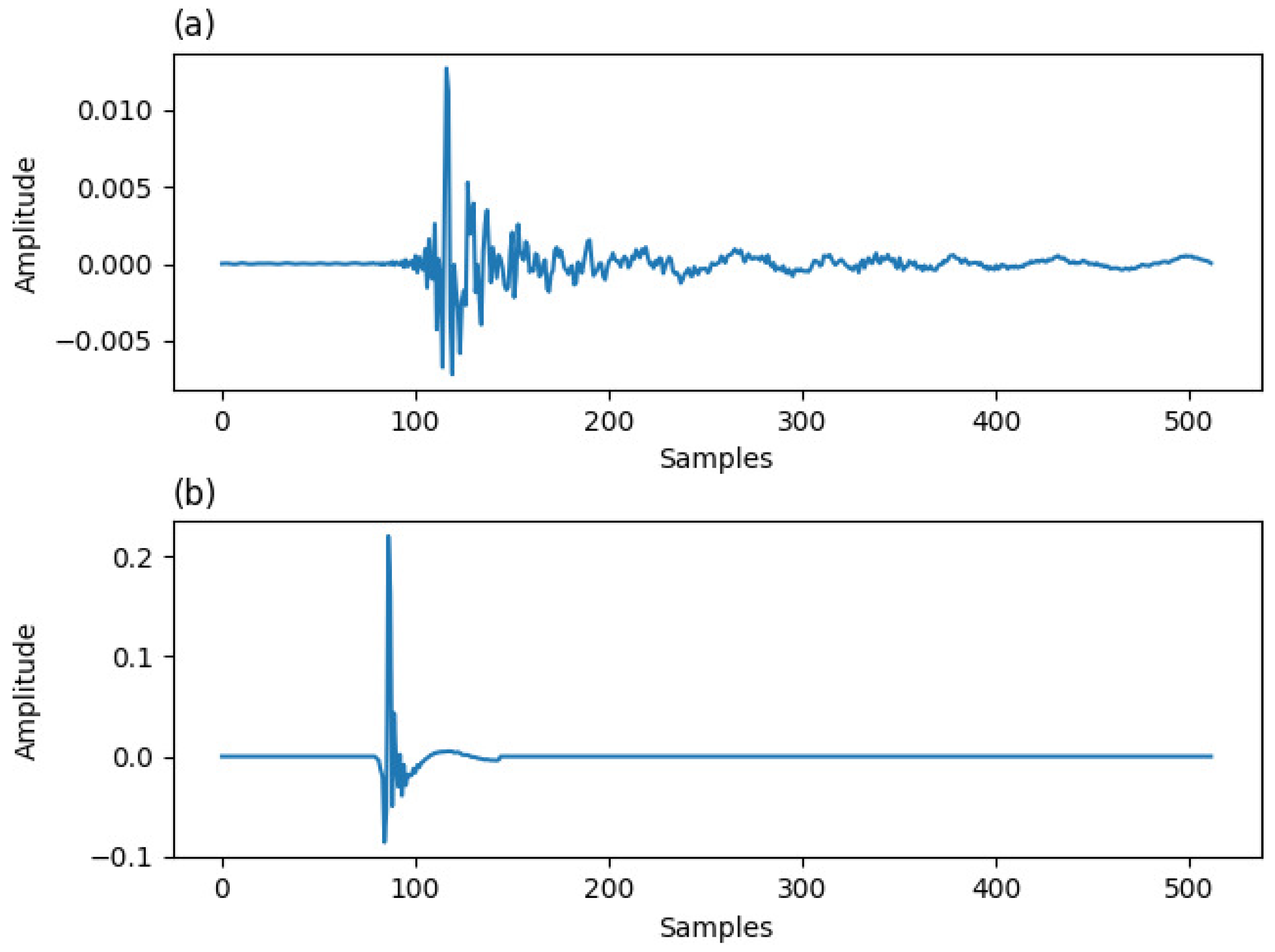
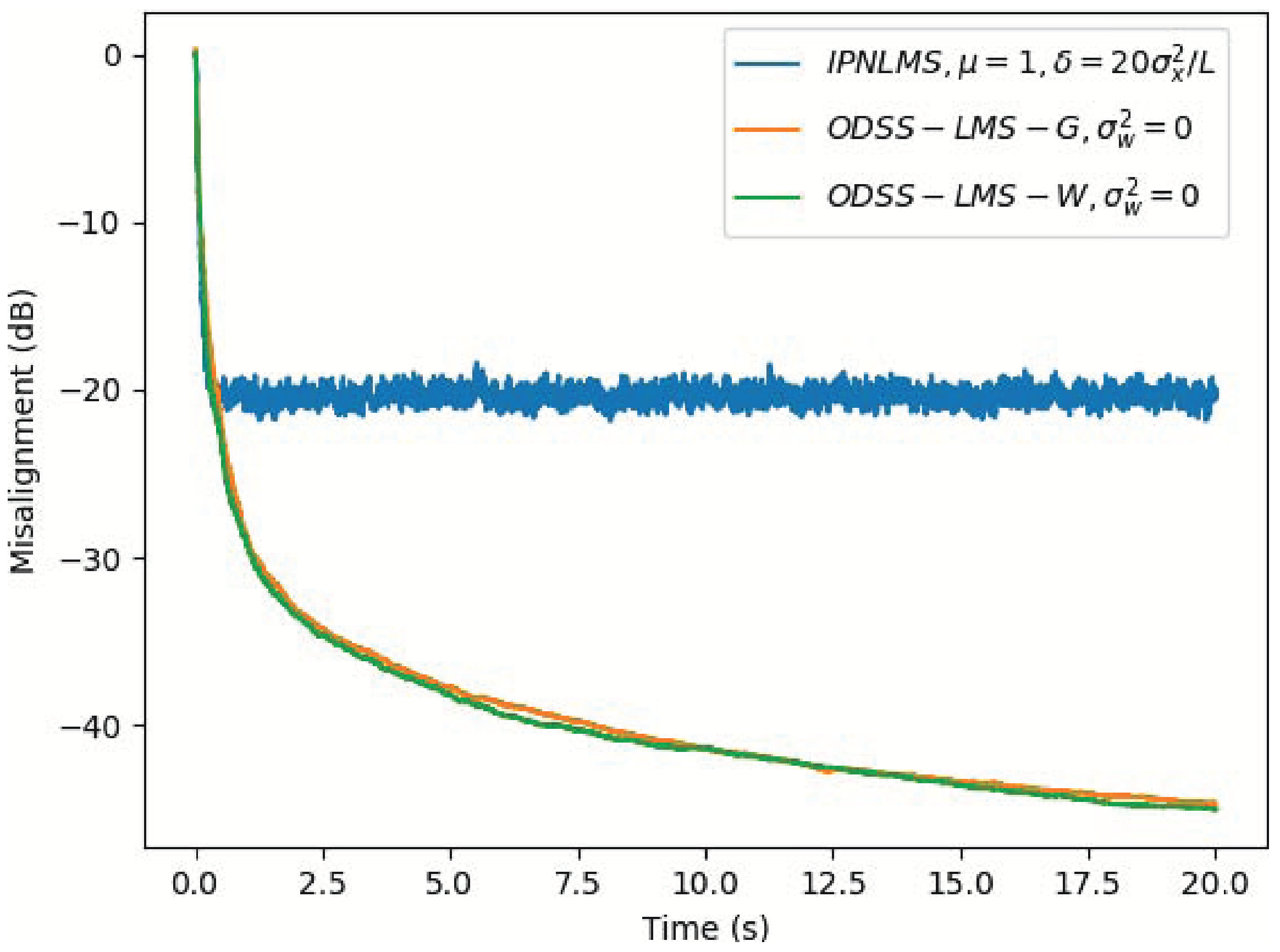
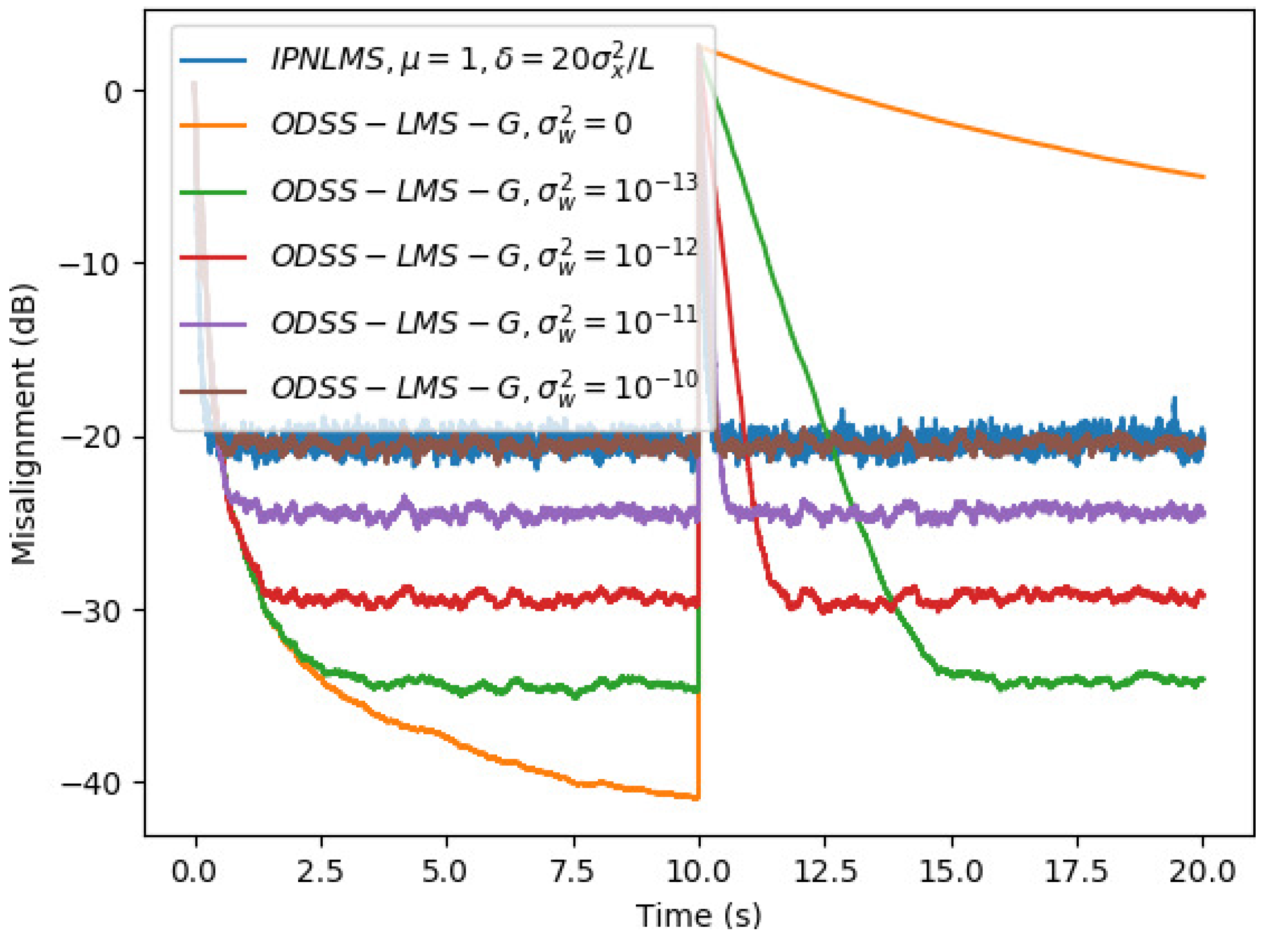
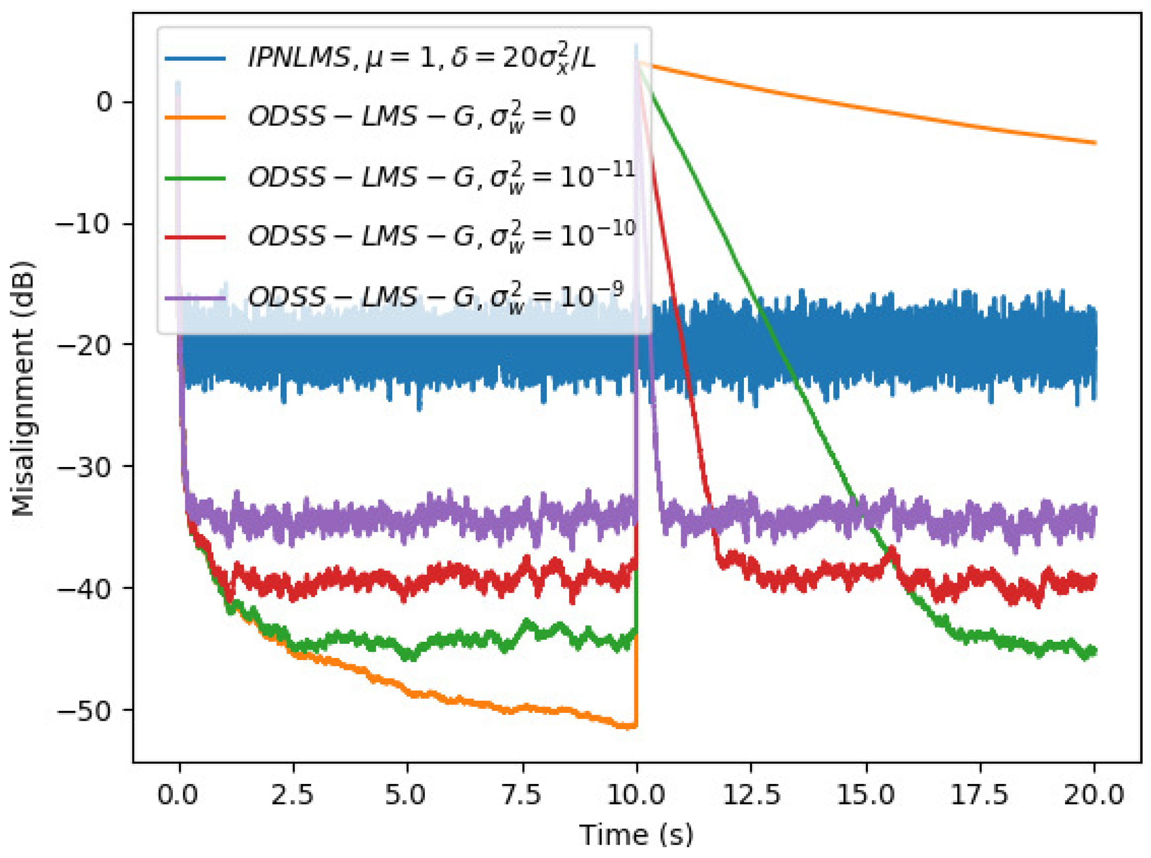
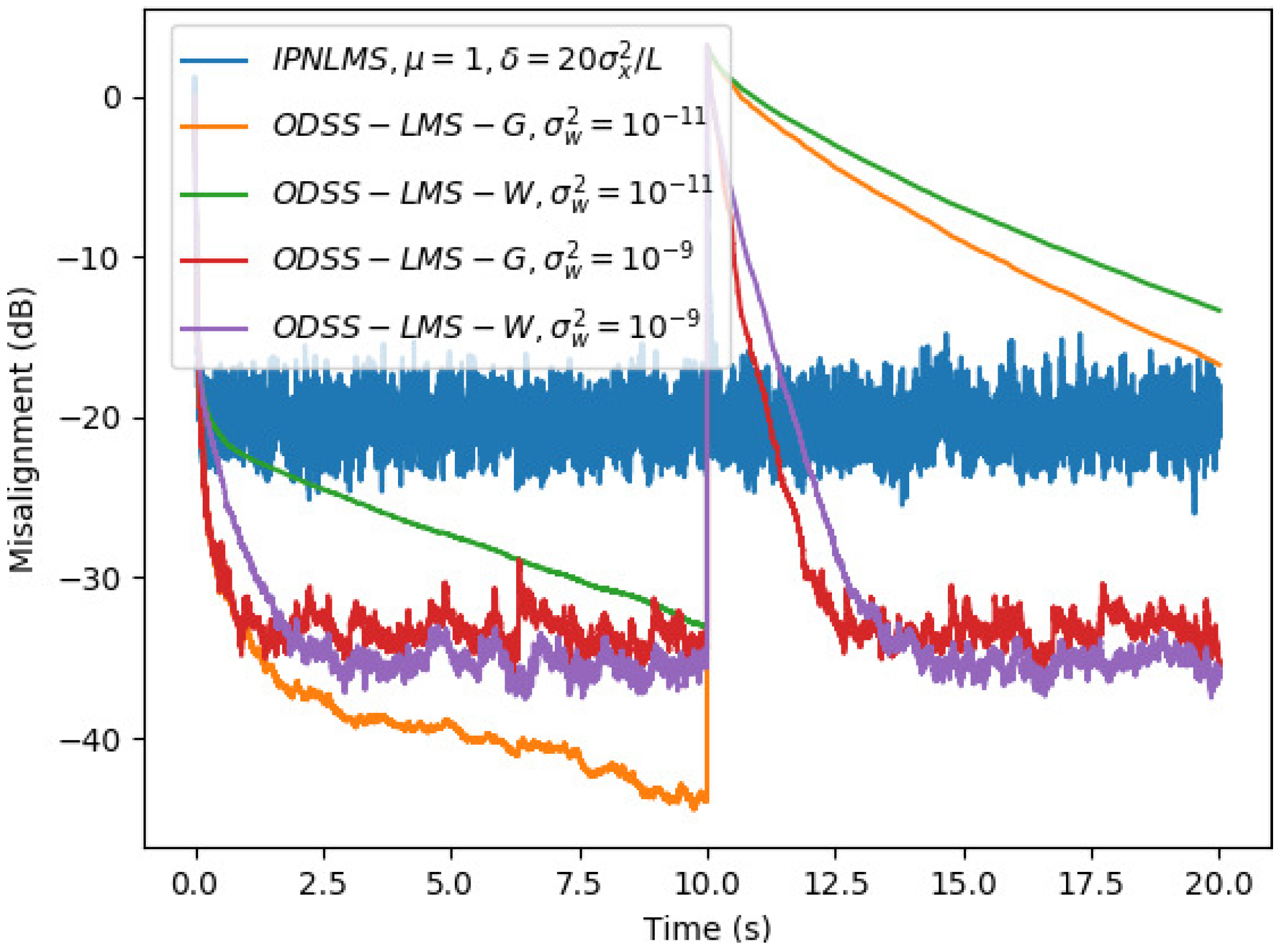
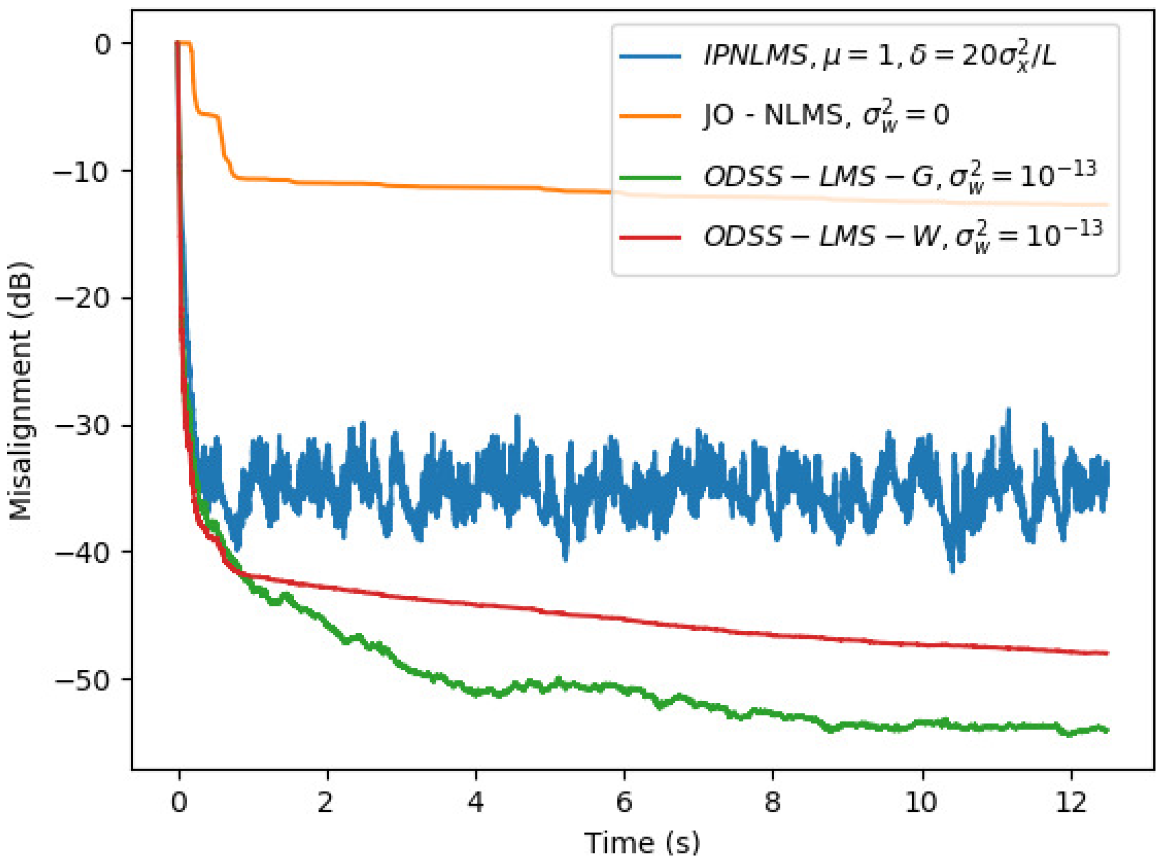
5. Simulation Results

The experiments are performed in the context of echo cancellation configuration using an acoustic impulse response and a sparse echo path from ITU-T G168 Recommendation [25] (padded with zeros). The echo paths have 512 coefficients and the same number is used for the adaptive filter, i.e., $L=512$. The sparseness measure based on the ${\ell }_1$ and ${\ell }_2$ norms [26] of the acoustic echo path is ${\xi }_{12}=0.6130$, while for the network echo path it is ${\xi }_{12}=0.8969$. The impulse responses used in our simulations are shown in Figure 1. In these scenarios, the sampling rate is 8 kHz. In this context, the unknown system is the echo path and the adaptive filter should estimate it. The output signal is corrupted by an independent white Gaussian noise with the signal-to-noise ratio (SNR) set to $\mathrm{SNR}={\sigma }_y^2/{\sigma }_v^2=20\mathrm{dB}$, where ${\sigma }_y^2=\mathrm{E}\left[y^2\left(n\right)\right]$. We assume that the power of this noise, ${\sigma }_v^2$, is known. The input signal, $x\left(n\right)$, is either a white Gaussian noise, an AR(1) process generated by filtering a white Gaussian noise through a first-order system $1/(1-\beta z^{-1})$, with $\beta =0.8,0.9$, or a speech sequence. The performance measure is the normalized misalignment in dB, defined as $20{\log }_{10}[{∥\mathbf{w}\left(n\right)-\widehat{\mathbf{w}}\left(n\right)∥}_2/{∥\mathbf{w}\left(n\right)∥}_2]$. The proposed algorithms are compared with the IPNLMS algorithm [4] (since, in general, it outperforms the NLMS algorithm) and also with the JO-NLMS algorithm [24] (using constant values of the parameter ${\sigma }_w^2$).

Figure 1. Echo paths used in simulations. (a) acoustic echo path and (b) network echo path (which is adapted from G168 Recommendation [25].)

In the first experiment, the acoustic echo path is involved. The system is considered time-invariant with ${\sigma }_w^2=0$. The ODSS-LMS-W and ODSS-LMS-G algorithms are compared with the IPNLMS algorithm in Figure 2, where the input signal is a white Gaussian noise. Thus, we confirm that relations (19), (24), and (26) are equivalent to (27), (28), and (29), respectively, in case of white Gaussian noise as an input signal. For the same convergence rate as the IPNLMS algorithm, the normalized misalignment of the proposed algorithms is definitely much lower.

Figure 2. Normalized misalignment of the IPNLMS, ODSS-LMS-G, and ODSS-LMS-W algorithms, where ${\sigma }_w^2=0$, the input signal is a white Gaussian noise, $L=512$, and SNR = 20 dB. The unknown system is the acoustic echo path.

In the context of acoustic echo cancellation, the tracking capability of the algorithm is an important aspect. Unfortunately, the acoustic path can rapidly change during the communication. Therefore, in Figure 3, the ODSS-LMS-G algorithm is analyzed for different values of ${\sigma }_w^2$ in a scenario where the input signal is a white Gaussian noise. The echo path change has been simulated by shifting the impulse response to the right (by 10 samples) in the middle of the experiment. In this scenario, the importance of the variance ${\sigma }_w^2$ is highlighted. The misalignment is much lower for low values of ${\sigma }_w^2$ and is dimmed for high values of this parameter (e.g., ${\sigma }_w^2={10}^{-10}$). Moreover, the variance of system noise indicates the need of a compromise between low misalignment and tracking capability (e.g., for ${\sigma }_w^2=0$, the ODSS-LMS-G algorithm tracks the optimal solution in a slow manner).

Figure 3. Normalized misalignment of the IPNLMS and ODSS-LMS-G algorithms for different values of ${\sigma }_w^2$. Echo path changes at time 10 s. The input signal is a white Gaussian noise, $L=512$, and SNR = 20 dB. The unknown system is the acoustic echo path.

Furthermore, we analyze the behavior of the ODSS-LMS-G algorithm for the identification of the sparse network echo path. Figure 4 outlines that the convergence rate is much faster than in the acoustic echo cancellation scenario, and the normalized misalignment decreases with at least 12 dB for all values of ${\sigma }_w^2$ as well.

Figure 4. Normalized misalignment of the IPNLMS and ODSS-LMS-G algorithms for different values of ${\sigma }_w^2$. Echo path changes at time 10 s. The input signal is a white Gaussian noise, $L=512$, and SNR = 20 dB. The unknown system is the network echo path.

Beyond this, the simulations are performed considering a stationary correlated input signal. In the context of acoustic echo cancellation configuration, Figure 5 shows the performance of the IPNLMS, JO-NLMS, ODSS-LMS-G, and ODSS-LMS-W algorithms in a scenario where the input signal is an AR(1) process, with $\beta =0.9$. It can be observed that, for high values of ${\sigma }_w^2$, it takes control in Equations (19), (24), (26) and (27)–(29) through $\mathbf{\Gamma }\left(n\right)$, and both ODSS-LMS algorithms behave similarly.

Figure 5. Normalized misalignment of the IPNLMS, JO-NLMS, ODSS-LMS-G, and ODSS-LMS-W algorithms for different values of ${\sigma }_w^2$. The input signal is an AR(1) process, with $\beta =0.9$, $L=512$, and SNR = 20 dB. The unknown system is the acoustic echo path.

Next, the ODSS-LMS-G and ODSS-LMS-W algorithms are analyzed for different values of ${\sigma }_w^2$ in a tracking scenario, where the input signal is an AR(1) process, with $\beta =0.8$. In Figure 6, the unknown system is represented by the sparse network path. The echo path changes in the same manner as in Figure 3. Up to a certain point, the ODSS-LMS-G algorithm deals better with correlated signal as input. We can remark on the lower normalized misalignment in case of ODSS-LMS-G algorithm for low values of ${\sigma }_w^2$, while the tracking capability is affected due to the lack of the initial estimation process. Even so, the tracking could be improved if the variance of the system noise is increased.

Figure 6. Normalized misalignment of the IPNLMS, ODSS-LMS-G, and ODSS-LMS-W algorithms for different values of ${\sigma }_w^2$. Echo path changes at time 10 s. The input signal is an AR(1) process, with $\beta =0.8$, $L=512$, and SNR = 20 dB. The unknown system is the network echo path.

In Figure 7, we compare the IPNLMS, ODSS-LMS-G, and ODSS-LMS-W algorithms for different values of ${\sigma }_w^2$ in an acoustic echo cancellation scenario, where the input signal is an AR(1) process with $\beta =0.9$. As in the scenario from Figure 6, the effect of ${\sigma }_w^2$ is attenuated with its increase. Therefore, the need of a variable ${\sigma }_w^2$ parameter arises. Low values of ${\sigma }_w^2$ will lead to a good compromise between fast initial convergence and low misalignment, while high values will keep alive the tracking capability. This issue will be addressed in future works, by targeting a variable parameter to this purpose.

Figure 7. Normalized misalignment of the IPNLMS, ODSS-LMS-G, and ODSS-LMS-W algorithms for different values of ${\sigma }_w^2$. Echo path changes at time 10 s. The input signal is an AR(1) process, with $\beta =0.9$, $L=512$, and SNR = 20 dB. The unknown system is the acoustic echo path.

Finally, in Figure 8, we compare the ODSS-LMS algorithms in a network echo cancellation scenario, where the input signal is a speech sequence. Again, we remark on the good performance of the ODSS-LMS-G algorithm with a highly correlated (and nonstationary) input signal.

Figure 8. Normalized misalignment of the IPNLMS, JO-NLMS, ODSS-LMS-G, and ODSS-LMS-W algorithms. The input signal is a speech sequence, $L=512$, and SNR = 20 dB. The unknown system is the network echo path.

6. Conclusions

Starting from the LMS algorithm, we developed an optimized differential step-size algorithm in order to update the adaptive filter coefficients. Our approach is developed in the context of a state-variable model and follows an optimization criterion based on the minimization of MSD. We derived a general algorithm valid for any input signal, ODSS-LMS-G, together with a simplified version for white Gaussian input signal, ODSS-LMS-W. The ODSS-LMS-G algorithm presents a high complexity (e.g., $O\left(L^3\right)$) due to matrix manipulations, while the complexity of the ODSS-LMS-W algorithm is $O\left(L\right)$. Nevertheless, they can be considered as benchmark versions for performance analysis. Their performance is highlighted in Section 5, emphasizing the features of the optimized step-size. An important parameter of the algorithm is ${\sigma }_w^2$, which should be tuned to address the compromise between low misalignment and fast tracking. In this context, it would be useful to find a variable parameter. Experiments demonstrate that the ODSS-LMS-G algorithm can be a benchmark in system identification, while the ODSS-LMS-W algorithm could be a possible candidate for field-programmable gate array (FPGA) applications, if the input signal is less correlated.

References

- Widrow, B. Least-Mean-Square Adaptive Filters; Haykin, S.S., Widrow, B., Eds.; Wiley: Hoboken, NJ, USA, 2003. [Google Scholar]
- Duttweiler, D.L. Proportionate normalized least-mean-squares adaptation in echo cancelers. IEEE Trans. Speech Audio Process. 2000, 8, 508–518. [Google Scholar] [CrossRef]
- Gay, S.L. An efficient, fast converging adaptive filter for network echo cancellation. In Proceedings of the Conference Record of Thirty-Second Asilomar Conference on Signals, Systems and Computers (Cat. No.98CH36284), Pacific Grove, CA, USA, 1–4 November 1998; pp. 394–398. [Google Scholar]
- Benesty, J.; Gay, S.L. An improved PNLMS algorithm. In Proceedings of the 2002 IEEE International Conference on Acoustics, Speech, and Signal Processing, Orlando, FL, USA, 13–17 May 2002. [Google Scholar]
- Deng, H.; Doroslovački, M. Proportionate adaptive algorithms for network echo cancellation. IEEE Trans. Signal Process. 2006, 54, 1794–1803. [Google Scholar] [CrossRef]
- Das Chagas de Souza, F.; Tobias, O.J.; Seara, R.; Morgan, D.R. A PNLMS algorithm with individual activation factors. IEEE Trans. Signal Process. 2010, 58, 2036–2047. [Google Scholar] [CrossRef]
- Liu, J.; Grant, S.L. Proportionate adaptive filtering for block-sparse system identification. IEEE/ACM Trans. Audio Speech Lang. Process. 2016, 24, 623–630. [Google Scholar] [CrossRef]
- Gu, Y.; Jin, J.; Mei, S. ℓ0 norm constraint LMS algorithm for sparse system identification. IEEE Signal Process. Lett. 2009, 16, 774–777. [Google Scholar]
- Loganathan, P.; Khong, A.W.H.; Naylor, P.A. A class of sparseness-controlled algorithms for echo cancellation. IEEE Trans. Audio Speech Lang. Process. 2009, 17, 1591–1601. [Google Scholar] [CrossRef]
- Li, Y.; Wang, Y.; Sun, L. A proportionate normalized maximum correntropy criterion algorithm with correntropy induced metric constraint for identifying sparse systems. Symmetry 2018, 10, 683. [Google Scholar] [CrossRef]
- Rusu, A.G.; Ciochină, S.; Paleologu, C. On the step-size optimization of the LMS algorithm. In Proceedings of the 42nd International Conference on Telecommunications and Signal Processing, Budapest, Hungary, 1–3 July 2019; pp. 168–173. [Google Scholar]
- Ciochină, S.; Paleologu, C.; Benesty, J.; Grant, S.L.; Anghel, A. A family of optimized LMS-based algorithms for system identification. In Proceedings of the 2016 24th European Signal Processing Conference (EUSIPCO), Budapest, Hungary, 29 August–2 September 2016; pp. 1803–1807. [Google Scholar]
- Enzner, G.; Buchner, H.; Favrot, A.; Kuech, F. Acoustic echo control. In Academic Press Library in Signal Processing; Academic Press: Cambridge, MA, USA, 2014; Volume 4, pp. 807–877. [Google Scholar]
- Shin, H.-C.; Sayed, A.H.; Song, W.-J. Variable step-size NLMS and affine projection algorithms. IEEE Signal Process. Lett. 2004, 11, 132–135. [Google Scholar]
- Benesty, J.; Rey, H.; Rey Vega, L.; Tressens, S. A nonparametric VSS-NLMS algorithm. IEEE Signal Process. Lett. 2006, 13, 581–584. [Google Scholar] [CrossRef]
- Park, P.; Chang, M.; Kong, N. Scheduled-stepsize NLMS algorithm. IEEE Signal Process. Lett. 2009, 16, 1055–1058. [Google Scholar] [CrossRef]
- Huang, H.-C.; Lee, J. A new variable step-size NLMS algorithm and its performance analysis. IEEE Trans. Signal Process. 2012, 60, 2055–2060. [Google Scholar] [CrossRef]
- Song, I.; Park, P. A normalized least-mean-square algorithm based on variable-step-size recursion with innovative input data. IEEE Signal Process. Lett. 2012, 19, 817–820. [Google Scholar] [CrossRef]
- Isserlis, L. On a formula for the product-moment coefficient of any order of a normal frequency distribution in any number of variables. Biometrika 1918, 12, 134–139. [Google Scholar] [CrossRef]
- Iqbal, M.A.; Grant, S.L. Novel variable step size NLMS algorithms for echo cancellation. In Proceedings of the 2008 IEEE International Conference on Acoustics, Speech and Signal Processing, Las Vegas, NV, USA, 31 March–4 April 2008; pp. 241–244. [Google Scholar]
- Paleologu, C.; Ciochină, S.; Benesty, J. Variable step-size NLMS algorithm for under-modeling acoustic echo cancellation. IEEE Signal Process. Lett. 2008, 15, 5–8. [Google Scholar] [CrossRef]
- Strassen, V. Gaussian Elimination is not Optimal. Numer. Math. 1969, 13, 354–356. [Google Scholar] [CrossRef]
- Coppersmith, D.; Winograd, S. Matrix multiplication via arithmetic progressions. J. Symb. Comput. 1990, 9, 251–280. [Google Scholar] [CrossRef]
- Ciochină, S.; Paleologu, C.; Benesty, J. An optimized NLMS algorithm for system identification. Signal Process. 2016, 118, 115–121. [Google Scholar] [CrossRef]
- ITU. Digital Network Echo Cancellers, ITU-T Recommendation G 168; ITU: Geneva, Switzerland, 2002. [Google Scholar]
- Hoyer, P.O. Non-negative matrix factorization with sparseness constraints. J. Mach. Learn. Res. 2001, 49, 1208–1215. [Google Scholar]
© 2019 by the authors. Licensee MDPI, Basel, Switzerland. This article is an open access article distributed under the terms and conditions of the Creative Commons Attribution (CC BY) license (http://creativecommons.org/licenses/by/4.0/).