A Quantum-Behaved Neurodynamic Approach for Nonconvex Optimization with Constraints

Abstract

This paper presents a quantum-behaved neurodynamic swarm optimization approach to solve the nonconvex optimization problems with inequality constraints. Firstly, the general constrained optimization problem is addressed and a high-performance feedback neural network for solving convex nonlinear programming problems is introduced. The convergence of the proposed neural network is also proved. Then, combined with the quantum-behaved particle swarm method, a quantum-behaved neurodynamic swarm optimization (QNSO) approach is presented. Finally, the performance of the proposed QNSO algorithm is evaluated through two function tests and three applications including the hollow transmission shaft, heat exchangers and crank–rocker mechanism. Numerical simulations are also provided to verify the advantages of our method.

1. Introduction

Constrained optimization problems arise in many scientific and engineering applications including robot control [1], regression analysis [2], economic forecasting [3], filter design [4] and so on. In many real-time applications, the optimization problems are often subject to complex and time-varying nature, which makes it difficult to compute global optimal solutions in real time using traditional numerical optimization techniques [4,5], such as Lagrange methods, descent methods and penalty function methods. A promising approach for handling these optimization problems is to employ neurodynamic optimization which is available for hardware implementation and possesses parallel and distributed computing ability. However, as pointed out in [6], the dynamic behaviors of a neural network could change drastically and become unpredictable, when applying neurodynamic optimization to deal with general nonconvex optimization problems. To compute global optimal solutions in such optimization problems, one solution is resorting to strategies in the meta-heuristics research field.

Recently, neurodynamic optimization based on recurrent neural networks has attracted much focus in solving various linear and nonlinear optimization problems. The essence of such neurodynamic optimization approaches is fundamentally different from those of iterative numerical algorithms such as the sequential programming method and interior point algorithms. The gradient method has been widely used in optimization problems [7,8]. Recurrent neural networks are also based on the gradient method and many other methods have been used to improve recurrent neural networks such as dual neural network [9,10], projection neural network [11], delayed neural network [12], weight-constrained neural networks [3,13] and so on. Some researchers focused on improving the performance of neural networks. Leung et al. [14] addressed a high-performance feedback neural network for solving convex nonlinear programming problems. Nazemi [15] explored a high performance neural network model to solve chance constrained optimization problem. Some researchers give different forms of neural networks for specific problems. Mansoori et al. presented a kind of recurrent neural network to solve quadratic programming problems and nonlinear programming problems with fuzzy parameters in [16,17]. Xia and Kamel presented a cooperative projection neural network to solve the least absolute deviation problems with general linear constraints [18]. Che and Wang presented a two-timescale duplex neurodynamic system for constrained biconvex optimization in [19]. For some special nonconvex and nonsmooth problems, some achievements have been made in neurodynamic optimization. Based on projection method and differential inclusions, Yang et al. [20] proposed a generalized neural network. In [21], a one-layer recurrent projection neural network was utilized for solving pseudoconvex optimization problems with general convex constraints. Li et al. [22] provided a one-layer recurrent neural network based on an exact penalty function method for solving nonconvex optimization problems subject to general inequality constraints. Bian et al. [23] proposed a one-layer recurrent neural network for solving a class of nonsmooth, pseudoconvex optimization problems with general convex constraints.

Despite great progresses of neurodynamic optimization approaches in solving optimization problems with convex or some pseudoconvex functions with constraints, it is difficult to find global optimal solutions for the optimization problems with more nonconvex functions. In addition, many neural networks seems inadequate when dealing with constrained optimization problems containing multiple local minima. As one of population-based evolutionary computation approaches, the well-known particle swarm optimization (PSO) introduced by by Kennedy and Eberhart [24] is a popular meta-heuristic method for global optimization with multimodal objective functions. In the PSO algorithm, a simple velocity and displacement model to adjust the position according to the group optimal value and its own optimal value. It has strong global search ability and robustness. However, the PSO algorithm has at least three shortcomings. Firstly, it has been proved by Frans in [25] that, when the number of iterations tends to infinity, the traditional PSO algorithm can not converge to the global optimal solution with probability $100\%$. Secondly, in the PSO algorithm, the velocity of particles has an upper limit to ensure that particles can aggregate and avoid divergence, which limits the search space of particles and thus makes the algorithm ineffective to jump out of local optimal solutions. Thirdly, as the evolution equation of the PSO algorithm is based on a set of simple state equations of velocity and position, which makes the randomness and swarm intelligence relatively low. Due to its simple calculation, easy implementation, and few control parameters, many improved PSO algorithms have been to overcome the drawbacks (e.g., see [26,27,28]). Yan et al. [6] presented a collective neurodynamic optimization approach by combining the traditional PSO algorithm and a projection neural network to solve nonconvex optimization problems with box constraints. Later, Yan et al. [29] apply an adaptive PSO algorithm together with a one-layer recurrent neural network to solve nonconvex general constrained optimization problems.

Among the improved PSO algorithms, the quantum-behaved particle swarm optimization (QPSO) algorithm introduced in [30] is also one promising alternate, which describes particle behavior with probability. Compared with the traditional PSO algorithm, the QPSO algorithm has certain advantages in global optimization and speed of convergence. The convergence proof of QPSO is also given in [27]. Applying the QPSO algorithm for global search intermittently by incorporating a novel feedback neural network for local search in a hybrid mode can be a good choice.

In this paper, we propose a quantum-behaved neurodynamic swarm optimization (QNSO) approach combined with an efficient neural network and the QPSO algorithm to solve the nonconvex optimization problems with constraints. We improve an efficient feedback neural network proposed in [14] and prove the global convergence of the neural network for a class of nonconvex optimization problems. Inspired by [6,14,29], we employ the feedback neural network and present a quantum-behaved neurodynamic swarm approach for solving the nonconvex optimization problems with inequality constraints efficiently. The proposed QNSO approach combining the QPSO algorithm [30] and the feedback neural network is applied to deal with constrained optimization problems with multiple global minima. Compared with the methods in [6,29], it shows a better convergence performance. Both numerical examples and practical applications are provided to demonstrate the effectiveness of the QNSO approach.

This paper is organized as follows. In Section 2, a constrained optimization problem is described and some theoretical analysis of an improved neural network is given. In Section 3, combined with the QPSO algorithm and the proposed neural network, the QNSO approach is developed for solving the constrained optimization problems. In Section 4, we perform experiments on two multimodal functions to demonstrate the performance of the QNSO algorithm. In Section 5, we apply the QNSO method to the optimization problems of the hollow transmission shaft, heat exchangers and crank–rocker mechanism. Finally, Section 6 concludes the paper.

2. Problem Statement and Model Description

Consider the following constrained optimization problem given by

$$\begin{array}{c}\begin{array}{cc}\hfill min& f\left(x\right),\hfill \\ \hfill \mathrm{subject}\mathrm{to}& g_i\left(x\right)\le 0,i=1,2,\cdots ,m,\hfill \end{array}\end{array}$$

(1)

where $x\in {\mathbb{R}}^n$ is the decision vector, $f:{\mathbb{R}}^n\to \mathbb{R}$ is a continuously differentiable function, $g_i:{\mathbb{R}}^n\to \mathbb{R}$ ($i=1,2,\cdots ,m$) are continuously differentiable functions, denoting the inequality constraints. $f\left(x\right)$ and $g_i\left(x\right)$ are not necessarily convex. The feasible region $\mathrm{\Omega }=\{x\in {\mathbb{R}}^n:g_i\left(x\right)\le 0,i=1,2,\cdots ,m\}$ is assumed to be a nonempty set.

Denote $g\left(x\right)={(g_1\left(x\right),g_2\left(x\right),\dots ,g_m\left(x\right))}^{\top }$. Then, the problem (1) can be written as

$$\begin{array}{c}\begin{array}{cc}\hfill \min & f\left(x\right),\hfill \\ \hfill \mathrm{subject}\mathrm{to}& g\left(x\right)\le 0.\hfill \end{array}\end{array}$$

(2)

Let $M_1$ be a lower bound of the optimal value of $f\left(x^{\ast }\right)$ in the problem (1), i.e., $M_1\le f\left(x^{\ast }\right)$, where $x^{\ast }$ is an optimal solution of (1). Denote $d(x,M_1)=f\left(x\right)-M_1$ and $F(x,M_1)=0.5d(x,M_1)(d(x,M_1)+|d(x,M_1)\left|\right)$. Consider an energy function

$$E\left(x\right)=F(x,M_1)+\gamma \left(g{\left(x\right)}^{\top }\mathrm{sgn}(g\left(x\right)+|g\left(x\right)\left|\right)\right),$$

(3)

where $\gamma >0$ is a penalty parameter, and $\mathrm{sgn}(·)$ is the sign function.

Then, inspired by [14,22], we construct the following feedback neural network for minimizing $E\left(x\right)$

$$\begin{array}{cc}\hfill \dot{x}=& -\nabla E\left(x\right)\hfill \\ \hfill =& -\nabla F(x,M_1)-\gamma \left(\nabla g{\left(x\right)}^{\top }\mathrm{sgn}(g\left(x\right)+|g\left(x\right)\left|\right)\right).\hfill \end{array}$$

(4)

Remark 1.

In [14], Leung et al. proposed the energy function $G(x,M_1)=F(x,M_1)+\frac{1}{2}g{\left(x\right)}^{\top }(g\left(x\right)-|g\left(x\right)\left|\right)+\frac{1}{2}{\Vert Ax-b\Vert }^2$ for the convex nonlinear programming problem

$$\begin{array}{cc}min& f\left(x\right),\\ subject\mathrm{to}& g\left(x\right)\ge 0,\\ & Ax=b.\end{array}$$

In fact, for some equality constraint $h\left(x\right)=0$, one can transform the equality constraint into inequality constraints $-h\left(x\right)\le 0$ and $h\left(x\right)\le 0$. The energy function $E\left(x\right)$ in (3) contains a penalty parameter γ. Such a penalty γ can strengthen the constraints and make the results converge into the constraints more efficiently in optimization problems with inequality constraints. In addition, as we will show later, the penalty parameter γ makes the neural network feasible to fit in the network model for solving some nonconvex problems in [22].

To derive the convergence results of the feedback neural network (4), we first introduce the following definitions.

Definition 1.

[22] Suppose that f is a differentiable function and defined on an open convex set $M\subset {\mathbb{R}}^n$. Then, f is quasiconvex if $a,b\in M,f\left(a\right)\ge f\left(b\right)\Rightarrow \nabla f{\left(a\right)}^{\top }(b-a)\le 0$.

Definition 2.

[22] Suppose that f is a differentiable function and defined on an open convex set $M\subset {\mathbb{R}}^n$. Then, f is pseudoconvex if $a,b\in M,f\left(a\right)>f\left(b\right)\Rightarrow \nabla f{\left(a\right)}^{\top }(b-a)<0$.

Theorem 1.

If $f\left(x\right)$ in (2) is a pseudoconvex function, then $F(x,M_1)$ in (3) is also a pseudoconvex function.

Proof of Theorem 1.

Let us rewrite $F(x,M_1)=0.5d(x,M_1)(d(x,M_1)+|d(x,M_1)\left|\right)$ as

$$F(x,M_1)=\left\{\begin{array}{cc}d{(x,M_1)}^2,\hfill & \hfill d(x,M_1)\ge 0,\\ 0,\hfill & \hfill d(x,M_1)<0.\end{array}\right.$$

By definition of $d(x,M_1)$, i.e., $d(x,M_1)=f\left(x\right)-M_1$, we have

$$\nabla F(x,M_1)=\left\{\begin{array}{cc}2d(x,M_1)\nabla f\left(x\right),\hfill & \hfill d(x,M_1)\ge 0,\\ 0,\hfill & \hfill d(x,M_1)<0,\end{array}\right.$$

(5)

and

$$F(x_1,M_1)-F(x_2,M_1)=\left\{\begin{array}{cc}d{(x_1,M_1)}^2-d{(x_2,M_1)}^2,\hfill & \hfill d(x_1,M_1)\ge 0,d(x_2,M_1)\ge 0,\\ d{(x_1,M_1)}^2,\hfill & \hfill d(x_1,M_1)\ge 0,d(x_2,M_1)<0,\\ -d{(x_2,M_1)}^2,\hfill & \hfill d(x_1,M_1)<0,d(x_2,M_1)\ge 0,\\ 0,\hfill & \hfill d(x_1,M_1)<0,d(x_2,M_1)<0.\end{array}\right.$$

Note that $F(x_1,M_1)-F(x_2,M_1)>0$ holds when

$$F(x_1,M_1)-F(x_2,M_1)=\left\{\begin{array}{cc}d{(x_1,M_1)}^2-d{(x_2,M_1)}^2>0,\hfill & \hfill d(x_1,M_1)\ge 0,d(x_2,M_1)\ge 0,\\ d{(x_1,M_1)}^2>0,\hfill & \hfill d(x_1,M_1)\ge 0,d(x_2,M_1)<0.\end{array}\right.$$

Using the definition of $d(x,M_1)$ again, it follows that $F(x_1,M_1)-F(x_2,M_1)>0$ implies that both $d(x_1,M_1)>0$ and $f\left(x_1\right)>f\left(x_2\right)$ holds. Therefore, using the fact that $f\left(x\right)$ is a pseudoconvex function, $F(x_1,M_1)-F(x_2,M_1)>0$ also implies $\nabla f\left(x_1\right)(x_2-x_1)<0$. In addition, since $F(x_1,M_1)-F(x_2,M_1)>0$ implies $d(x_1,M_1)>0$, it follows from (5) that

$$\nabla F{(x_1,M_1)}^{\top }(x_2-x_1)=2d(x_1,M_1)\nabla f\left(x_1\right)(x_2-x_1)<0$$

if $F(x_1,M_1)-F(x_2,M_1)>0$. The proof is completed. □

Remark 2.

From the proof of Theorem 1, it should be noted that the function F is constructed as a semi-positive definition function and the term $\left|d\right(x,M_1\left)\right|$ can be seen as an adaptive adjustment function when computing the gradient of $E\left(x\right)$. That is, when $f\left(x\right)$ approaches $f\left(x^{\ast }\right)$, $d(x,M_1)$ becomes smaller and $\nabla f\left(x\right)$ plays a minor role in computing the gradient of $E\left(x\right)$; when $f\left(x\right)$ is far away from $f\left(x^{\ast }\right)$, $d(x,M_1)$ becomes larger and $\nabla f\left(x\right)$ plays an important role in computing the gradient of $E\left(x\right)$.

To establish a relationship between the feedback neural network (4) and the neural network in [22], we consider the following notion and lemmas.

Definition 3.

[29] (Clarke’s generalized gradient) The generalized gradient of f at x, denoted by $\partial f\left(x\right)$, is the convex hull of the set of limits of the form $lim\nabla f(x+l_i)$, where $l_i\to 0$ as $i\to \infty$.

Lemma 1.

[22] [Proposition 6] Let $g\left(x\right)$ be continuously differentiable. Then, $max\{0,g(x\left)\right\}$ is a regular function, its Clarke’s generalized gradient is

$$\partial max\{0,g(x\left)\right\}=\left\{\begin{array}{cc}\nabla g\left(x\right),\hfill & \hfill g\left(x\right)>0,\\ {\alpha }_g\nabla g\left(x\right),\hfill & \hfill g\left(x\right)=0,\\ 0,\hfill & \hfill g\left(x\right)<0,\end{array}\right.$$

where ${\alpha }_g\in [0,1]$.

Lemma 2.

[22] [Theorem 4] For the problem (1), if one of the following two conditions holds,

(a) 

$f\left(x\right)$ and $g_i\left(x\right)$, $i=1,2,\cdots ,m$ are convex functions;

(b) 

$f\left(x\right)$ is a pseudoconvex function and $g_i\left(x\right)$, $i=1,2,\cdots ,m$ are quasiconvex functions,

then, for a sufficiently small penalty factor $\sigma >0$, any state of the following recurrent neural network

$$\begin{array}{c}\dot{x}\in -\nabla f\left(x\right)-\frac{1}{\sigma }\partial \sum _{i=1}^{m}max\{0,g_i\left(x\right)\}\hfill \end{array}$$

(6)

converges to an optimal solution of problem (1).

Definition 4.

(KKT Point) For the problem (1), suppose that $f\left(x\right)$ : ${\mathbb{R}}^n\to \mathbb{R}$ is differentiable and $g_i\left(x\right)$ : ${\mathbb{R}}^n\to \mathbb{R},i=1,2,\cdots ,m$ are differentiable functions. If $(\overline{x},\overline{\mu })\in {\mathbb{R}}^n\times {\mathbb{R}}^m$ satisfies the following conditions:

$$\nabla f\left(\overline{x}\right)+{\overline{\mu }}^{\top }\nabla g\left(\overline{x}\right)=0,\overline{\mu }\ge 0,g\left(\overline{x}\right)\le 0,{\overline{\mu }}^{\top }g\left(\overline{x}\right)=0,$$

then $\overline{x}$ is said to be a KKT point of problem (1). The KKT conditions provide first-order necessary conditions for nonlinear programming problem and can be considered as local optimization points for programming problem.

Under some acceptable assumptions (see [22] for details), the following properties hold.

Proposition 1.

[22] [Theorem 1] When the penalty parameter σ is sufficiently small, then any state of (6) is guaranteed to be convergent to the feasible region in finite time and stay there thereafter.

Proposition 2.

[22] [Corollary 1] When the penalty parameter σ is sufficiently small, any state of the neural network (6) will converge to an equilibrium point $\overline{x}$ and any equilibrium point $\overline{x}$ of the neural network (6) corresponds to a KKT twofold $(\overline{x},\overline{\mu })$ of the problem (1).

Next, we claim that for the problem (1), the neural network (4) is a special form of neural network (6). Firstly, note that, to solve the the problem $minF(x,M_1)$ with the constraint $g\left(x\right)\le 0$, it is equivalent to solving the problem $minf\left(x\right)$ with the constraint $g\left(x\right)\le 0.$ Secondly, take ${\alpha }_g=0$ in Lemma 1, the neural network (4) can be written as

$$\begin{array}{ccc}\dot{x}\hfill & =\hfill & -\nabla F(x,M_1)-\gamma (\nabla g{\left(x\right)}^{\top }\mathrm{sgn}(g\left(x\right)+|g\left(x\right)\left|\right))\hfill \\ & =\hfill & -\nabla F(x,M_1)-\gamma \partial {\displaystyle \sum _{i=1}^m}max\{0,g_i\left(x\right)\}.\hfill \end{array}$$

(7)

Define $\sigma :=\frac{1}{\gamma }$ in (7). It follows that

$$\begin{array}{c}\dot{x}=-\nabla F(x,M_1)-\frac{1}{\sigma }\partial {\displaystyle \sum _{i=1}^m}max\{0,g_i\left(x\right)\},\hfill \end{array}$$

which is a special case of the neural network (6) in Lemma 2 if $F(x,M_1)$ has the same property of the function f in Lemma 2.

The following result shows the convergence property of the proposed neural network.

Theorem 2.

The neural network (4) converges to an optimal solution of problem (1) if there exists a large enough penalty parameter $\gamma >0$ and one of the following two conditions holds

(a) 

$f\left(x\right)$ and $g_i\left(x\right)$, $i=1,2,\cdots ,m$ are convex functions;

(b) 

$f\left(x\right)$ is a pseudoconvex function and $g_i\left(x\right)$, $i=1,2,\cdots ,m$ are quasiconvex functions.

Proof of Theorem 2.

Firstly, if condition (a) holds, it follows from [14] [Theorem 1] that $F(x,M_1)$ in (3) is also a convex function. Then, condition (a) in Lemma 2 holds. Secondly, if condition (b) holds, it follows from Theorem 1 that $F(x,M_1)$ in (3) is also a pseudoconvex function. Then, condition (b) in Lemma 2 holds. In addition, it follows from the above discussion that the neural network (4) fits in the form of neural network (6). Therefore, by Lemma 2, the proof is completed. □

Remark 3.

Theorem 2 shows that the proposed neural network (4) will converge to an optimal solution for some nonconvex optimization problems and (4) satisfies the properties in Propositions 1 and 2, that is, the neural network (4) can converge to the feasible region of the optimization problem in finite time and find a KKT point which is a local optimal point of the problem (1).

3. Quantum-Behaved Neurodynamic Swarm Approach

To solve the nonconvex programming problems with box constraints, a collective neurodynamic approach is proposed in [6], which can be seen as a combination of neurodynamic optimization and particle swarm optimization. In order to improve the convergence speed of the optimization algorithm, we explore a quantum-behaved neurodynamic approach combining the QPSO algorithm with the feedback neural network model (7) for nonconvex programming problems with general constraints. In the QPSO algorithm, each particle represents a position, which represents a potential optimal solution of optimization problem. Imitating the swarm intelligence behavior of animals, the renewal of particles is related to their optimal position and global optimal position. Unlike the basic PSO algorithm, the updating equation of particle position follows the quantum-behaved model. The QPSO algorithm has the aggregation of particles with the iteration, increases the intelligence of particle behavior, and makes the possible search range of particles wider. Therefore, the ability of global optimization increases.

Given q particles, define the position of the ith particle as $X_i=(X_{i1},X_{i2},$$\cdots ,X_{in})$, the individual best position of the ith particle as $P_i=(P_{i1},P_{i2},\cdots ,P_{in})$ and the best position of the swarm as $P_g=(G_1,G_2,\cdots ,G_n)$. The particle renewal equation of the QPSO algorithm is given by

$$\begin{array}{c}\begin{array}{c}\hfill X_{ij}(k+1)=p_{ij}\left(k\right)\pm \beta |C_j\left(k\right)-X_{ij}\left(k\right)|ln\frac{1}{{\eta }_{ij}\left(k\right)},\end{array}\end{array}$$

(8)

where

$$\begin{array}{c}\begin{array}{cc}\hfill p_{ij}\left(k\right)& ={\alpha }_j\left(k\right)P_{ij}\left(k\right)+[1-{\alpha }_j\left(k\right)]G_j\left(k\right)\hfill \\ \hfill C\left(k\right)& =(C_1\left(k\right),C_2\left(k\right),\cdots ,C_n\left(k\right))=\frac{1}{q}\sum _{i=1}^q{P}_i\left(k\right)\hfill \\ & =\frac{1}{q}\left(\sum _{i=1}^q{P}_{i1}\left(k\right),\sum _{i=1}^q{P}_{i2}\left(k\right),\cdots ,\sum _{i=1}^q{P}_{in}\left(k\right)\right)\hfill \end{array}\end{array}$$

and ${\alpha }_j\left(k\right),{\eta }_{ij}\left(k\right)$ are random numbers between $(0,1)$, $j\in \{1,2,\cdots ,n\}$, $i\in \{1,2,\cdots ,q\}$, $\beta$ is an adjustable parameter, $p_{ij}\left(k\right)$ is the center of attraction potential field of $X_{ij}(k+1)$. $C\left(k\right)$ is the average optimal position of particle. The iteration stops when the maximum number of iterations is reached or the given conditions is achieved.

Note that, despite of its excellent global optimization ability, the QPSO algorithm lacks the ability for constraint processing and deep local searching. Inspired by neurodynamic optimization, during the local search process, we apply the feedback neural network to optimize each particle and improve the search efficiency. Next, we explore the QNSO approach to deal with constrained optimization problems, where the QPSO algorithm is applied to adjust the initial conditions of the feedback neural network at each local search phrase.

The steps of the QNSO algorithm are summarized as follows:

Step 1:

Initialize the position of particles.

Step 2:

Initialize the individual best position $P_i$ of the ith particle, $i=1,2,\cdots ,q$ and the global best position $P_g$ of the particle swarm.

Step 3:

Each particle reaches a local optimal solution based on the feedback neural network (7).

Step 4:

Update the individual best position $P_i$ of the ith particle, $i=1,2,\cdots ,q$ and the global best position $P_g$ of the particle swarm.

Step 5:

Update the position of each particles based on (8).

Step 6:

Repeat Step 3 to Step 5 before reaching the given conditions.

Following the description in Section 2, we simply consider the energy function in (3) as the fitness value of the QPSO algorithm. Then, the individual best position $P_i$ of the ith particle is updated according to

$$P_i\left(k\right)=\left\{\begin{array}{cc}{X}_i\left(k\right),\hfill & \mathrm{when}E\left(X_i\left(k\right)\right)<E\left(P_i(k-1)\right),\hfill \\ P_i(k-1),\hfill & \mathrm{when}E\left(X_i\left(k\right)\right)\ge E\left(P_i(k-1)\right),\hfill \end{array}\right.$$

(9)

where $k-1$ and k represent the $k-1$th iteration and kth iteration, respectively. The global best position $P_g$ of the particle swarm is updated by

$$\begin{array}{c}{P}_g\left(k\right)=\underset{1\le i\le q}{min}\left\{E\left(P_i\left(k\right)\right)\right\}.\end{array}$$

(10)

Remark 4.

The fitness value of the QNSO algorithm could be different from the energy function of the neural network. A large γ may bring a better performance as it effectively restricts particles to diverge beyond the feasible region.

QNSO can always find the accurate local minimum of each particle within one iteration. Compared with general global optimization algorithms (such as PSO), when the number of local minimum is small, QNSO is extremely insensitive to heuristic parameters; when the number of local minimum is large, the QNSO algorithm needs sufficient divergence ability of heuristic parameters to jump out of local minimum. In other words, appropriately larger $\beta$ in QPSO can be more suitable for the QNSO algorithm.

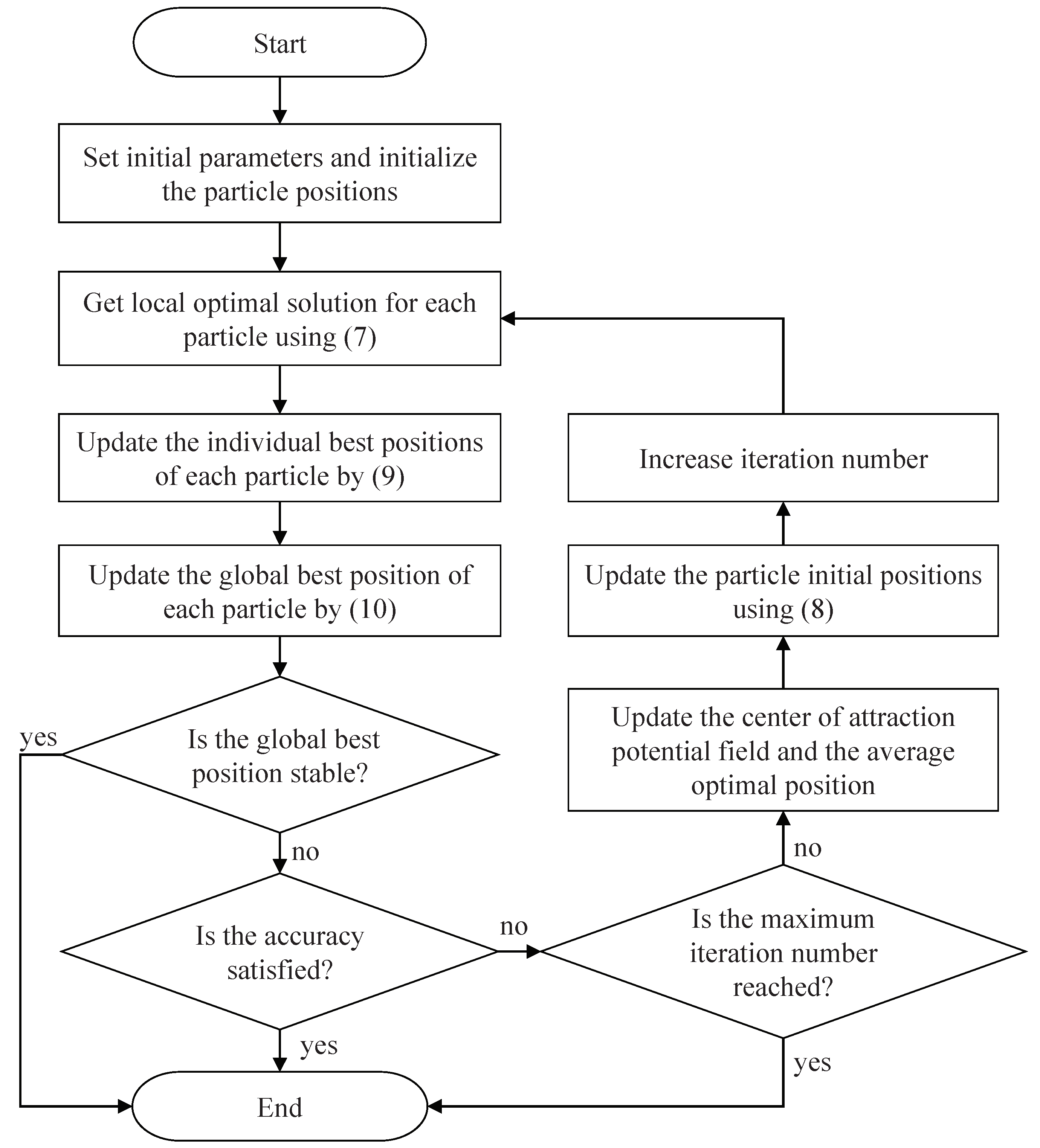
Detailed steps of the QNSO algorithm are given in Algorithm 1. During local search process, the feedback neural network in the algorithm is applied to solve the local optimization problem with constraints. The QPSO algorithm is applied to perform global search process. Therefore, the advantages of the QPSO algorithm and the feedback neural network can complement each other. The flow chart of QNSO is shown in Figure 1.

Figure 1. Flow chart of the QNSO algorithm.

Algorithm 1 QNSO Algorithm.

1: Set the swarm size q, parameter $\beta$, tolerance error precision $\epsilon$, the maximum number $K_{max}$ of iterations, the expected cost function value $E_e$, the lower bound of cost function $M_1$ and the initial step $k=0$. 2: Initialize the position $X_i\in {\mathbb{R}}^n$ of particles, $i=1,2,\cdots ,q,$ using uniform random distribution, and get the initial individual best positions and global best position. 3: Carry out the following feedback neural network to obtain a local optimal solution for each particle: $$\begin{array}{c}ϵ\dot{x}=-\nabla F(x,M_1)-\gamma \partial {\displaystyle \sum _{i=1}^q}\left(max\{0,g_i\left(x\right)\}\right),\hfill \end{array}$$ where $ϵ>0$ is a scaling parameter which is introduced to accelerate the convergence rate of the neural network. 4: Update the individual best position $P_i$ of the ith particle, $i=1,2,\cdots ,q$ and the global best position $P_g$ of the particle swarm using $$P_i\left(k\right)=\left\{\begin{array}{cc}{X}_i\left(k\right),\hfill & \mathrm{when}E\left(X_i\left(k\right)\right)<E\left(P_i(k-1)\right),\hfill \\ P_i(k-1),\hfill & \mathrm{when}E\left(X_i\left(k\right)\right)\ge E\left(P_i(k-1)\right),\hfill \end{array}\right.$$ and $$\begin{array}{c}{P}_g\left(k\right):=(G_1,G_2,\cdots ,G_n)=\underset{1\le i\le q}{min}\left\{E\left(P_i\left(k\right)\right)\right\}.\end{array}$$ 5: Update the position $X_i(k+1)$ of each particle, that is, the initial conditions of the feedback neural network, using the following the renewal equations: $$\begin{array}{c}\begin{array}{cc}\hfill p_{ij}\left(k\right)& ={\alpha }_j\left(k\right)P_{ij}\left(k\right)+[1-{\alpha }_j]G_j\left(k\right),\hfill \\ \hfill C\left(k\right)& =\frac{1}{q}\sum _{i=1}^q{P}_i\left(k\right),\hfill \\ \hfill X_{ij}(k+1)& =p_{ij}\left(k\right)\pm \beta |C_j\left(k\right)-X_{ij}\left(k\right)|ln\frac{1}{{\eta }_{ij}\left(k\right)},\hfill \end{array}\end{array}$$ where $i=1,2,\cdots ,q,$$j=1,2,\cdots ,n$ and ${\alpha }_j\left(k\right)\sim U(0,1),$${\eta }_{ij}\left(k\right)\sim U(0,1)$.   6: The iteration stops if one of the following conditions is satisfied: (a) The algorithm reaches the maximum iteration value $K_{max}$.   (b) $|E\left(P_g\right)-E_e|<\epsilon$.   (c) $P_g$ stops updating for five consecutive iterations. Otherwise, set $k:=k+1$ and go to step 3.

4. Function Tests

In this section, we consider two multimodal benchmark problems, i.e., the constrained six-hump camel back function [6] and the constrained Rastrigrin function, to illustrate the proposed optimization approach. The first example is provided to verify the convergence performance of the proposed QNSO algorithm, while the second example is provided to demonstrate the constraint processing ability of the algorithm.

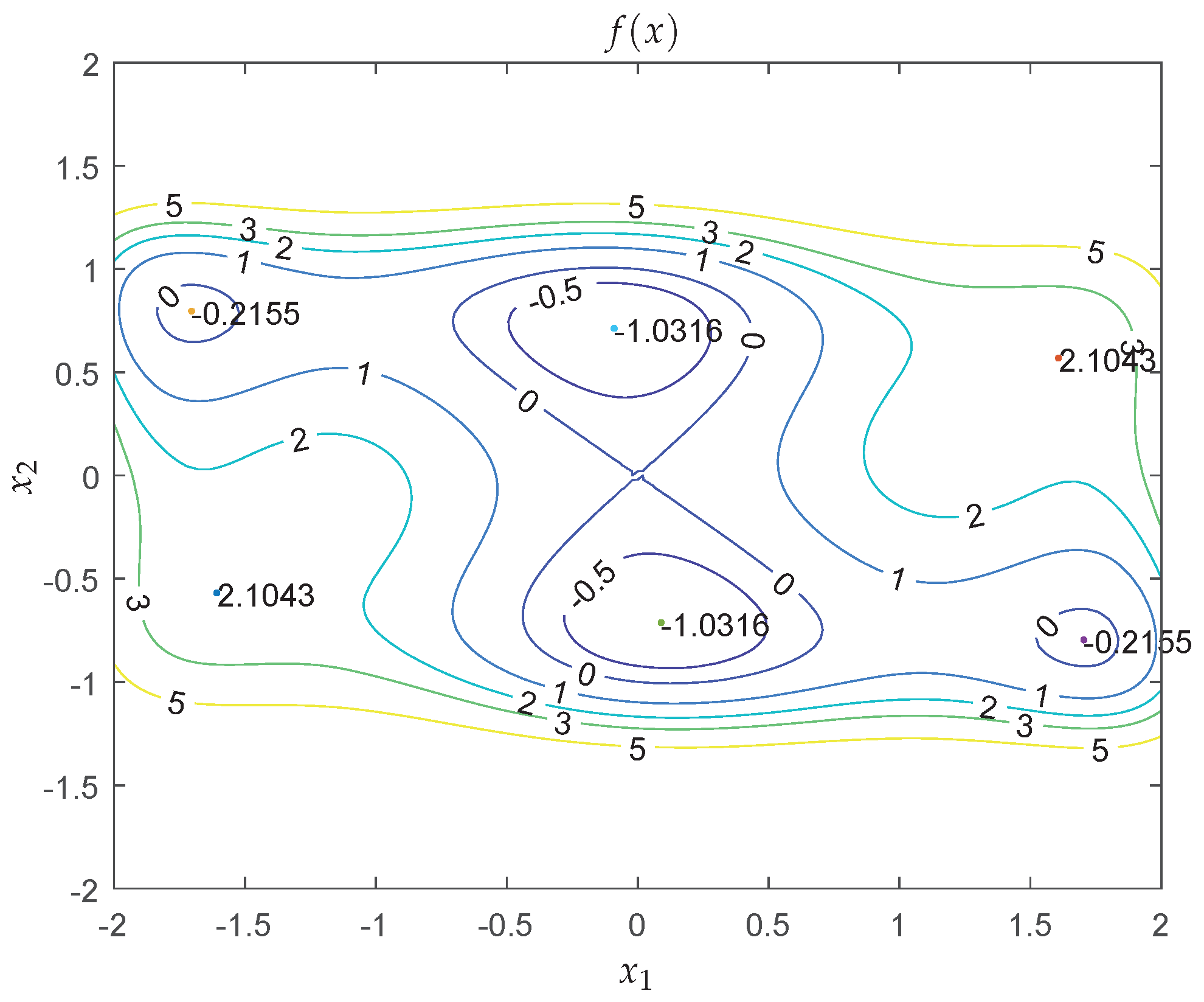
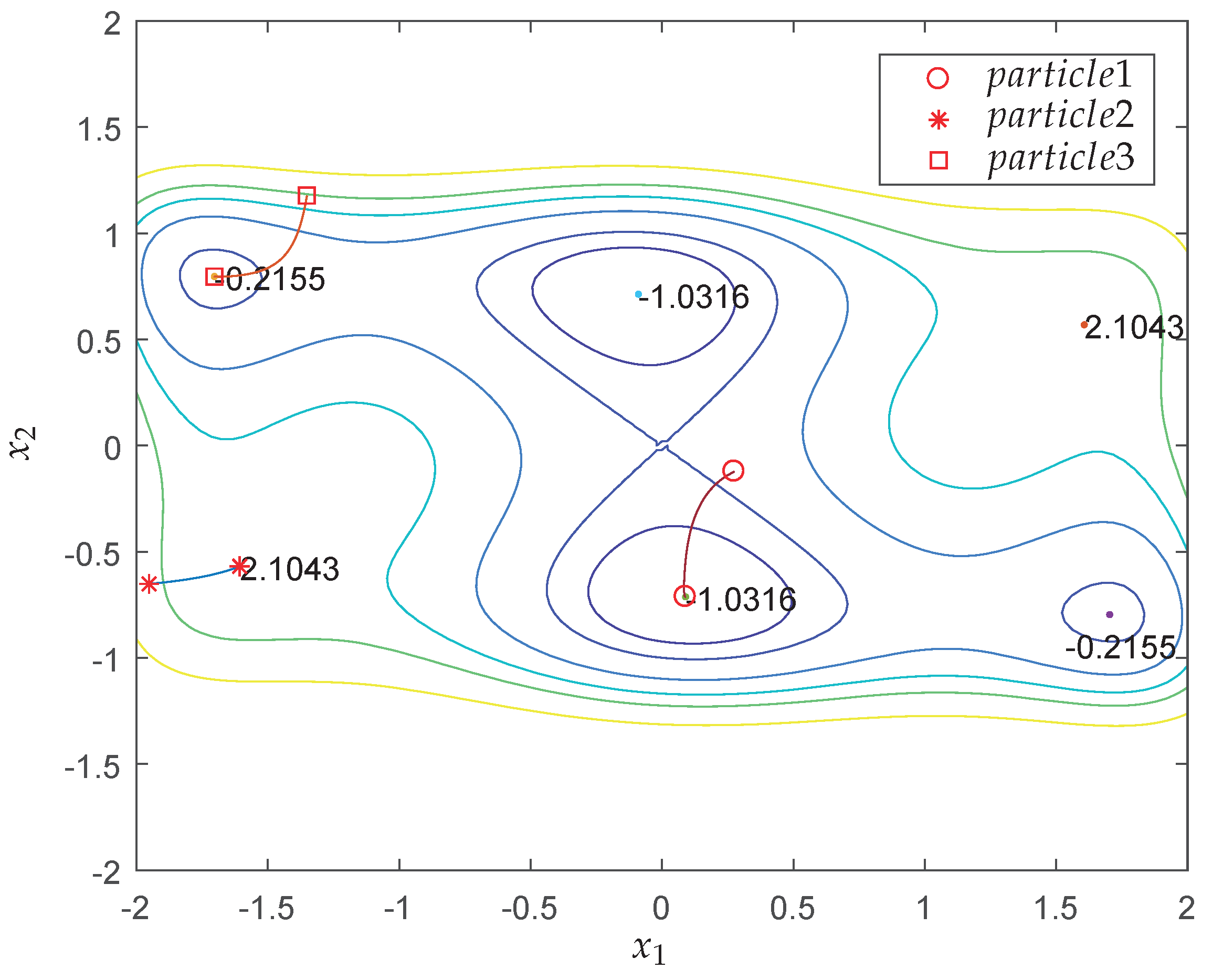
Example 1.

Consider the six-hump camel back function [6]

$$\begin{array}{cc}min& f(x_1,x_2)=(4-2.1x_1^2+\frac{x_1^4}{3})x_1^2+x_1{x}_2+4(x_2^2-1)x_2^2,\hfill \\ \mathrm{subject}\mathrm{to}& -2\le x_i\le 2,i=1,2.\hfill \end{array}$$

Figure 2 shows the contour map of the six-hump camel back function with box constraints. It is seen that there are multiple local minima in the area. In fact, the optimization problem has six minima

$$\left\{\begin{array}{c}f(-1.6071,-0.5687)=2.1043,\hfill \\ f(1.6071,0.5687)=2.1043,\hfill \\ f(-1.7036,0.7961)=-0.2155,\hfill \\ f(1.7036,-0.7961)=-0.2155,\hfill \\ f(0.0898,-0.7127)=-1.0316,\hfill \\ f(-0.0898,0.7127)=-1.0316.\hfill \end{array}\right.$$

Figure 2. Contour map of f in Example 1, where different color lines represent contours corresponding to different values of f.

Two of them are the global minima, located at $x^{\ast }=(-0.0898,0.7127)$ and $x^{\ast }=(0.0898,$$-0.7127)$, respectively. To carry out the QNSO algorithm, set swarm size $q=3$, parameter $\beta =\frac{1}{2}$, tolerance error precision $\epsilon ={10}^{-6}$, the maximum iteration number $K_{max}=10$, $M_1=-20,$ and $\gamma =1000$. Before performing the simulation, initialize the position $X_{ij}\in [-2,2]$ of particles, $i=1,2,3,$$j=1,2$, using uniform random distribution. After 50 experiments, we obtain the two global minima at every experiment. Except two experiments, the global minima are found at the first step iteration for most cases, which shows that the QNSO algorithm has a high efficiency and good accuracy to find the optimal solution for the problem in this example.

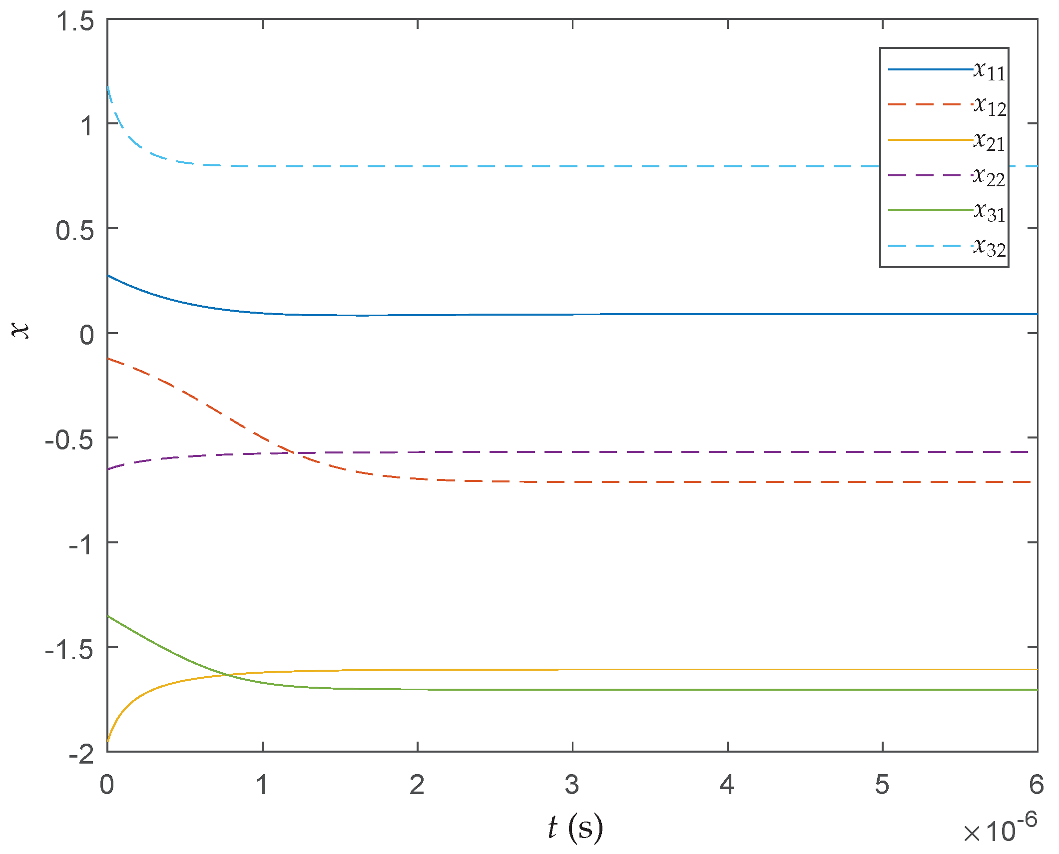
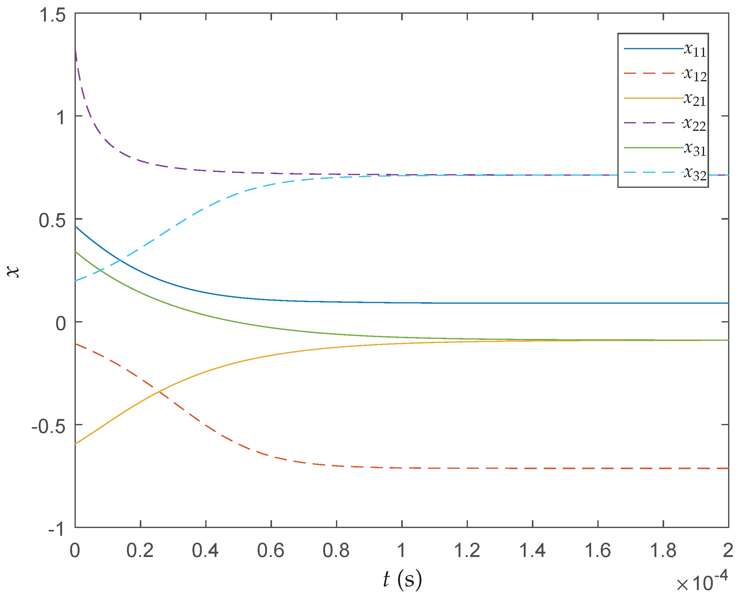
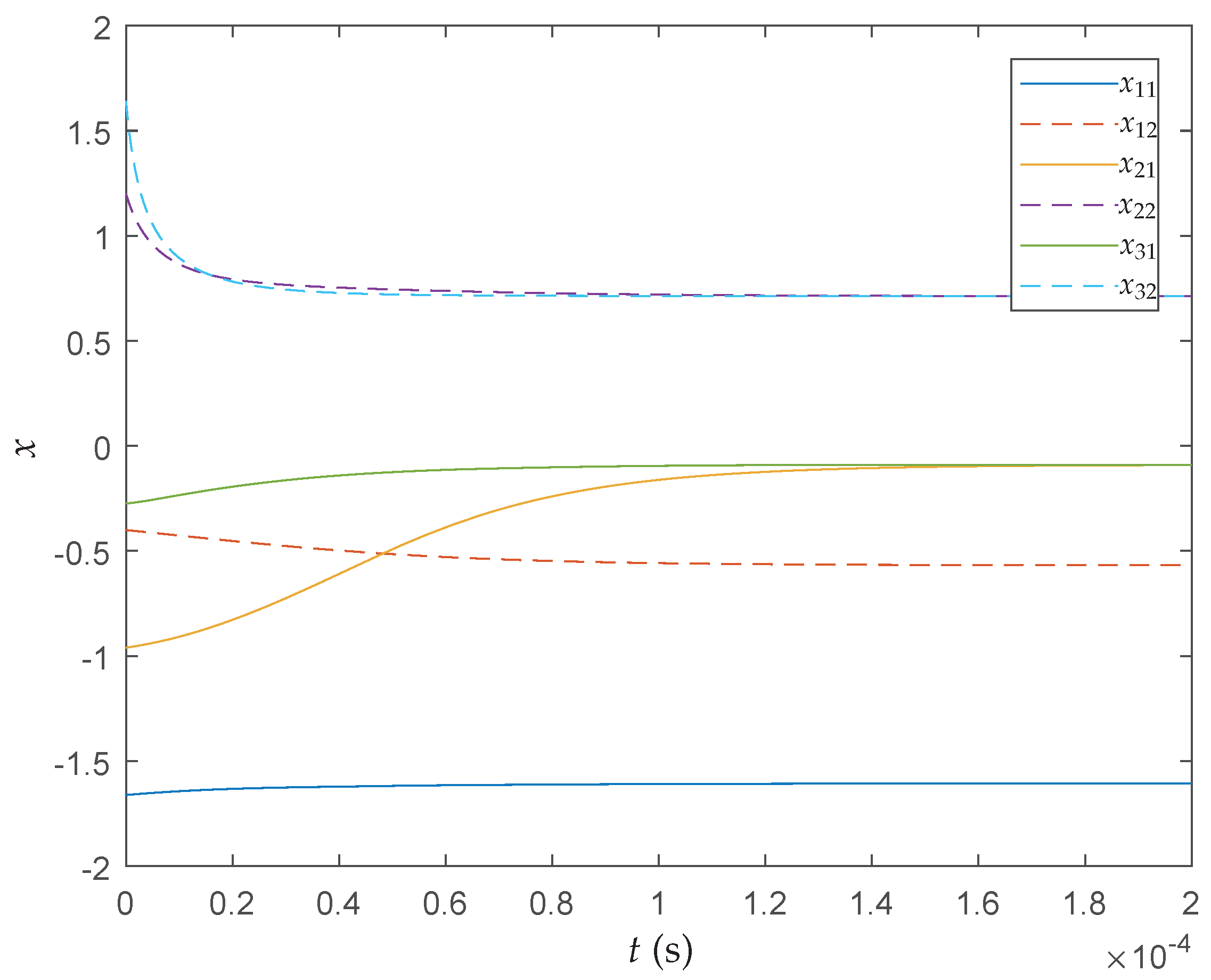
In order to verify the convergence efficiency of the proposed method, we compare the optimization results of the QNSO algorithm with the results derived by the approaches in [6,29]. For the neural networks in all the three methods, we take the scaling parameter $ϵ={10}^{-3}$. Figure 3, Figure 4 and Figure 5 show the convergence of the trajectory of the proposed neural network (7), the projection neural network in [6], and the recurrent neural network in [29] at the first iteration, respectively. As shown in the figures, each particle converges to its local optimum shortly. It can be seen that, among the three methods, the proposed neural network has the fastest convergence speed.

Figure 3. Convergence of the proposed neural network.

Figure 4. Convergence of the neural network in [6].

Figure 5. Convergence of the neural network in [29].

Figure 6 shows the behavior of particles in the search process by the proposed QNSO algorithm. The initial positions of particles are randomly selected. After one iteration, two particles reach the global minima along the direction perpendicular to the contour.

Figure 6. Moving trails of the three particles using the QNSO algorithm, where different color lines represent contours corresponding to different values of f and the corresponding values are shown in Figure 2.

Example 2.

Consider the optimization problem of the constrained Rastrigrin function described by

$$\begin{array}{cc}min\hfill & f\left(x\right)={\displaystyle \sum _{i=1}^n}(x_i^2-10cos\left(2\pi x_i\right)+10),\hfill \\ \mathrm{subject}\mathrm{to}\hfill & -6\le x_i\le 6,\hfill \\ & {\displaystyle \sum _{i=1}^n}{x}_i^2\ge 4.5,\hfill \end{array}$$

(11)

which has hundreds of local minima and many global minima for $n\ge 4$. Note that the origin, which is the global minimum point for unconstrained Rastrigrin function, is not within the feasible range. The complexity of this problem depends on the size of n and the number of minima increases exponentially with the increase of n.

To carry out the QNSO algorithm, set the initial parameters of QNSO algorithm: $M_1=0,\gamma =1000$, $\beta$ decreased from $0.9$ to $0.3$ on the course of the search, swarm size $q=20$, tolerance error precision $\epsilon ={10}^{-5}$, the maximum iteration number $K_{max}=500$. To establish a reference for comparison with the QNSO algorithm in this paper, we performed experiments with Rastrigrin function in $2,$ 4 and 10 dimensions, respectively. Some other optimization methods were also examined for performance comparisons, including the latest standard particle swarm optimization (SPSO) [31], the adaptive particle swarm optimization (APSO) [32], the random drift particle swarm optimization (RDPSO) [33], the firefly algorithm (FA) [34], the repair genetic algorithm (RGA) [35], the QPSO [30], and the method in [29]. We set swarm size $q=20$, tolerance error precision $\epsilon ={10}^{-5}$, the maximum iteration number $K_{max}=500$ for all the tested methods. Standard normal distribution was used in RGA as mutation operator. The parameters for QPSO were the same as those in this paper. Other parameters for SPSO, APSO, FA, RDPSO and RGA were the same as those recommended in [31,32,33,34,35] and these methods used the same fitness value (3) with a large $\gamma ={10}^6$ to keep optimizations within the feasible range.

Table 1, Table 2 and Table 3 show the computational results, where the best result, the average result, the worst result, the standard deviation (Std.) result of $f\left(P_g\right)$, and the average number of iterations (No. of Iterations) over 50 experiments are provided. The optimum results are coarsened with boldface in these tables. Obviously, when the particles and the iterations are limited, the general optimization algorithm has obvious deficiencies with the increase of the complexity of the problem, but the method in [29] and QNSO can obtain accurate optimal solutions with good robustness. QNSO requires the least iterations with a stable optimization efficiency as shown in Table 1 and Table 2.

Table 1. Comparing computational efficiency ($n=2$).

Methods	Best	Average	Worst	Std.	No. of Iterations
SPSO [31]	4.9751	4.9925	5.0594	0.0190	500
APSO [32]	4.9758	4.9978	5.0738	0.0211	500
FA [34]	4.9748	4.9748	4.9750	$3.6985\times {10}^{-5}$	481.5
RGA [35]	4.9748	5.0164	6.5421	0.7317	414.9
RDPSO [33]	4.9748	4.9774	4.9956	$5.7606\times {10}^{-3}$	450.56
QPSO [30]	4.9748	4.9749	4.9760	$2.6078\times {10}^{-4}$	327.92
[29]	4.9748	4.9748	4.9748	$4.39\times {10}^{-8}$	2.4
QNSO	4.9748	4.9748	4.9748	$\mathbf{3.151}\times {\mathbf{10}}^{-\mathbf{9}}$	1.3

Table 2. Comparing computational efficiency ($n=4$).

Methods	Best	Average	Worst	Std.	No. of Iterations
SPSO [31]	5.6356	6.8906	8.2099	0.65794	500
APSO [32]	5.1884	6.7265	8.0925	0.87531	500
FA [34]	4.9793	7.0177	20.9417	3.1047	500
RGA [35]	4.9748	5.0627	7.4586	0.45259	500
RDPSO [33]	4.9748	5.3332	9.0534	0.88538	472.26
QPSO [30]	4.9748	5.2261	5.9917	0.4433	468.6
[29]	4.9748	4.9748	4.9748	$5.8247\times {10}^{-7}$	5.34
QNSO	4.9748	4.9748	4.9748	$\mathbf{9.5127}\times {\mathbf{10}}^{-\mathbf{8}}$	4.18

Table 3. Comparing computational efficiency ($n=10$).

Methods	Best	Average	Worst	Std.	No. of Iterations
SPSO [31]	27.5833	39.7451	51.0513	6.2649	500
APSO [32]	23.8351	39.3527	50.4733	7.1493	500
FA [34]	30.3567	56.3786	81.7154	12.5423	500
RGA [35]	4.9754	4.9872	5.0509	0.01809	500
RDPSO [33]	4.9748	6.9563	13.2190	2.3012	500
QPSO [30]	4.9748	5.7736	8.9549	0.9786	495.7
[29]	4.9748	4.9748	4.9748	$1.5934\times {10}^{-6}$	12.54
QNSO	4.9748	4.9748	4.9748	$\mathbf{1.1478}\times {\mathbf{10}}^{-\mathbf{6}}$	14.3

5. Applications

In this section, three optimization problems in applications, including hollow transmission shaft [36], heat exchangers [37] and crank–rocker mechanism [36], are solved using the proposed QNSO algorithm.

Application 1.

(Hollow transmission shaft) Consider the hollow transmission shaft optimization problem in [36], where D and d are the outer diameter and inner diameter, $d=8$ mm, shaft length $L=3.6$ m. The power transmitted by the shaft is $P=7$ kW and the speed $n=1500\mathrm{r}/\min$. Shaft material density p = 7800 $\mathrm{kg}/{\mathrm{m}}^2$, shear modulus $S=81$ GPa, and allowable shear stress $\overline{\tau }=45$ MPa, allowable torsion angle per unit length $\overline{\phi }=1.5°$ m. The aim is to minimize the mass of the shaft under the limitations of torsional strength and torsional stiffness:

(1)

Decision variables and cost function

In this problem, there is only one decision variable $x:=D$. According to the design requirements, the optimization goal is to minimize the mass of the shaft that is, $f\left(x\right)=\frac{\pi }{4}\rho L(D^2-d^2)$.

(2)

Restrictions

(a)

Torsional strength condition is ${\tau }_{max}=\frac{T}{W_n}\le \overline{\tau },$ where T is the torque received by the round shaft, $T=9550\frac{P}{n}$, $W_n$ is the torsional section modulus, $W_n=\frac{\pi (D^4-d^4)}{16D}$.

(b)

Torsional stiffness condition is $\phi =\frac{T}{S{J}_p}\le \overline{\phi },$ where $\phi$ is unit length twist angle, G is shear modulus, $J_p$ is polar moment of inertia, $J_p=\frac{\pi (D^4-d^4)}{32}$.

(c)

Outer diameter minimum limit condition is $x\ge d.$

Following the above analysis, we summarize the optimization problem as follows:

$$\begin{array}{c}\begin{array}{cc}\hfill minf\left(x\right)=& \frac{\pi }{4}\rho L(x^2-d^2)\times {10}^{-6},\hfill \\ \hfill \mathrm{subject}\mathrm{to}{g}_1\left(x\right)=& d-x\le 0,\hfill \\ \hfill g_2\left(x\right)=& \frac{16xT\times {10}^9}{\pi (x^4-d^4)}-\overline{\tau }\times {10}^6\le 0,\hfill \\ \hfill g_3\left(x\right)=& \frac{32T\times {10}^3}{S\pi (x^4-d^4)}-\overline{\phi }\times \frac{\pi }{180}\le 0.\hfill \end{array}\end{array}$$

(12)

For the above problem (12), one can use the $fmincon$ function in Matlab to obtain a solution $x^{\ast }=21.6121$ mm with $f\left(x^{\ast }\right)=8.8896$ kg [36]. To carry out the QNSO algorithm, we set swarm size $q=5$, parameter $\beta =\frac{1}{2}$, tolerance error precision $\epsilon ={10}^{-6}$, the maximum iteration number $K_{max}=15$, $M_1=0,$ and $\gamma =1000$. The initial values of the position $X_i\in [8,100]$ of particles, $i=1,2,\cdots ,5,$ are randomly chosen. We perform 50 realizations and obtain an optimal solution $x^{\ast }=21.5965$ mm with $f\left(x^{\ast }\right)=8.8747$ kg, which is slightly better than that obtained in [36].

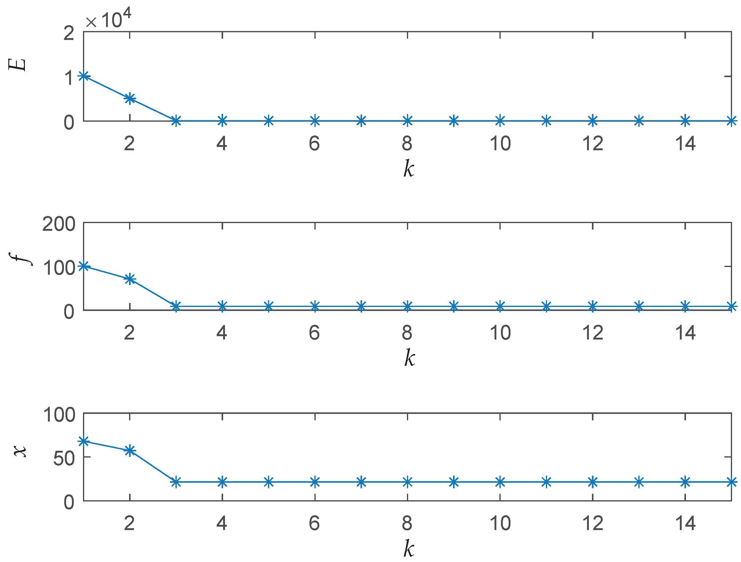
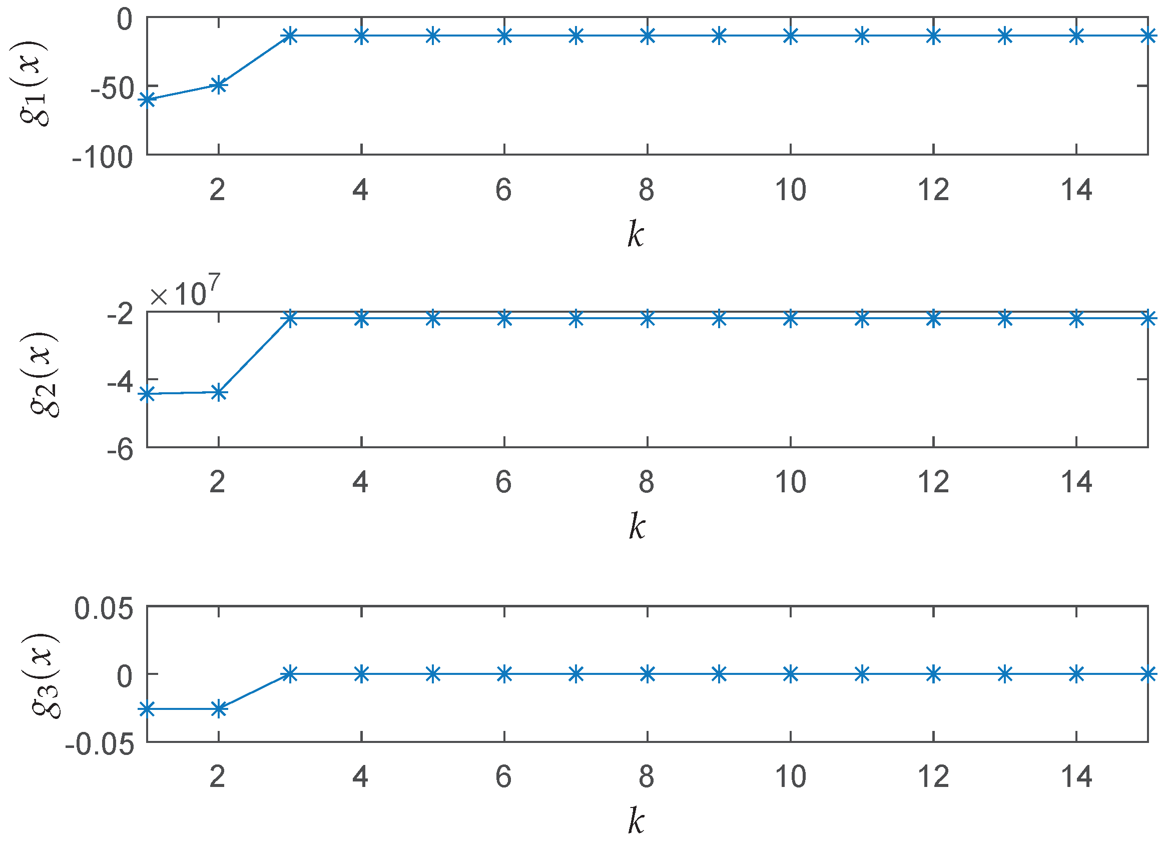
Figure 7 shows the iteration results of the energy function E, the cost function f and the solution x of the best particle among five particles. As seen from the results, the proposed algorithm successfully solves the optimization problem with a fast convergence speed and finds a relative ideal solution within five iterations. Figure 8 depicts the iteration results of the inequality constraint functions and illustrates the ability of the algorithm to deal with constraints. Table 4 shows the best result, the average result, the worst result, and the standard deviation result of $f\left(P_g\right)$ over 50 realizations.

Figure 7. Convergence results of E,f and x in Application 1.

Figure 8. Iteration results of $g_i\left(x\right)$ in Application 1, $i=1,2,3$.

Table 4. Statistical analysis of the results in Application 1.

Best	Average	Worst	Std.
8.8747	8.8759	8.8767	$6.62\times {10}^{-5}$

Application 2.

(Heat exchangers [37]) Consider three connected heat exchangers as shown Figure 9, which are used to heat a material temperature from ${100}^{\circ }$ to ${500}^{\circ }$. Let $m{c}_p={10}^5$, where m is the mass flow rate of the fluid and $c_p$ is the specific heat capacity of the fluid. The heat transfer coefficients of the three heat exchangers are $K_1=120$, $K_2=80$ and $K_3=40$, respectively. For simplicity, the temperature difference $▵t_m$ uses arithmetic mean value and the above values are obtained through dimensionless processing. The aim is to minimize the total heat transfer area by selecting the appropriate temperature.

Figure 9. Flow chart of heat exchangers.

The decision variables are $x={[T_1,T_2]}^{\top }$. The restrictions are given by $100\le T_1\le 300$ and $T_1\le T_2\le 400.$ It follows from the law of conservation of heat that

$$\begin{array}{c}\begin{array}{c}m{c}_p(T_1-100)=m{c}_p(300-T_3)\Rightarrow T_3=400-T_1,\hfill \\ m{c}_p(T_2-T_1)=m{c}_p(400-T_4)\Rightarrow T_4=400-T_2+T_1,\hfill \\ m{c}_p(500-T_2)=m{c}_p(600-T_5)\Rightarrow T_5=100-T_2.\hfill \end{array}\hfill \end{array}$$

The arithmetic mean values of temperature difference of heat exchangers are

$$\begin{array}{c}\begin{array}{c}▵t_{m1}=\frac{300-T_1+T_3-100}{2}=300-T_1,\hfill \\ ▵t_{m2}=\frac{400-T_2+T_4-T_1}{2}=400-T_2,\hfill \\ ▵t_{m3}=\frac{600-500+T_5-T_2}{2}=100.\hfill \end{array}\hfill \end{array}$$

Therefore, according to the design requirements, the cost function is obtained

$$f\left(x\right)=\frac{{10}^5(T_1-100)}{120(300-T_1)}+\frac{{10}^5(T_2-T_1)}{80(400-T_2)}+\frac{{10}^5(500-T_2)}{4000}.$$

To sum up, the optimization problem can be written as

$$minf\left(x\right)=\frac{{10}^5(x_1-100)}{120(300-x_1)}+\frac{{10}^5(x_2-x_1)}{80(400-x_2)}+\frac{{10}^5(500-x_2)}{4000},$$

$$\begin{array}{c}\begin{array}{cc}\hfill \mathrm{subject}\mathrm{to}& g_1\left(x\right)=100-x_1\le 0,\hfill \\ & g_2\left(x\right)=x_1-300\le 0,\hfill \\ & g_3\left(x\right)=x_1-x_2\le 0,\hfill \\ & g_4\left(x\right)=x_2-400\le 0.\hfill \end{array}\end{array}$$

(13)

In [37], the obtained minimum cost function value is $7049.4191$ by using sequence quadratic programming. To carry out the QNSO algorithm, we set swarm size $q=5$, parameter $\beta =\frac{1}{2}$, tolerance error precision $\epsilon ={10}^{-6}$, the maximum iteration number $K_{max}=6$, $M_1=0,$ and $\gamma =1000$. The initial values of the position $X_{ij}\in [0,400]$ of particles, $i=1,2,\cdots ,5,$$j=1,2,$ are randomly chosen. Since the problem is relatively simple, after performing the simulation, we can obtain the optimal solution at the first iteration almost every time. We perform 50 realizations and obtain the same results which are shown in Table 5. 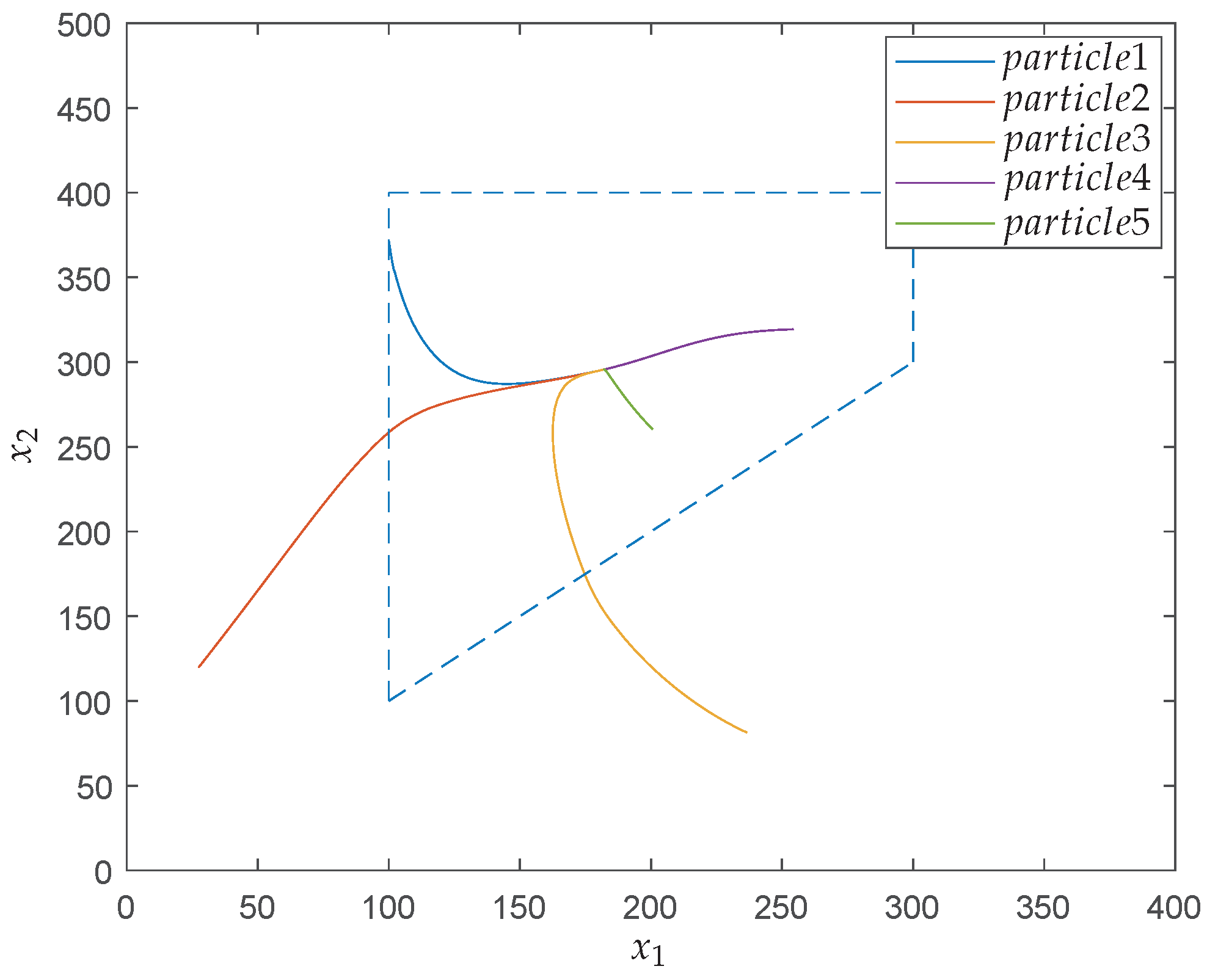Figure 10 shows the behavior of particles in the search process in the phase plot by the proposed QNSO algorithm. It can be found that all particles move into the feasible region and reach some local optimal solutions.

Table 5. Optimization results in Application 2.

$\mathit{f}\left({\mathit{x}}^{\ast }\right)$	${\mathit{x}}_1^{\ast }$	${\mathit{x}}_2^{\ast }$	${\mathit{g}}_1\left({\mathit{x}}^{\ast }\right)$	${\mathit{g}}_2\left({\mathit{x}}^{\ast }\right)$	${\mathit{g}}_3\left({\mathit{x}}^{\ast }\right)$	${\mathit{g}}_4\left({\mathit{x}}^{\ast }\right)$
7049.2493	182.0179	295.6012	−82.01787	−117.9821	−113.5834	−104.3988

Figure 10. Moving trails of the particles using the QNSO algorithm in Application 2 (dotted line: feasible region).

Application 3.

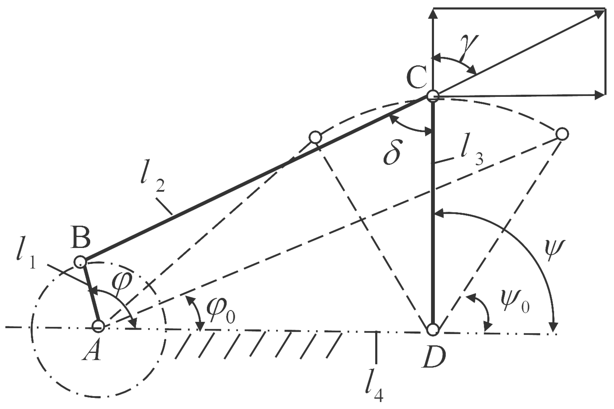
(Crank–rocker mechanism [36]) Consider a crank–rocker mechanism as shown in Figure 11. The anti-clockwise angle is calculated with the frame $AD$ as the baseline. ${\psi }_0$ and ${\phi }_0$ correspond to the position angles of the rocker and the crank respectively when the rocker is in the right limit position. The minimum transmission angle ${\gamma }_{min}$ is greater than ${45}^{\circ }$. The crank–rocker mechanism is required to be designed when the crank is transferred from ${\phi }_0$ to ${\phi }_0+\frac{\pi }{2}$ and the output angle $\psi$ of the rocker meets the following predetermined motion rules ${\psi }_s$: ${\psi }_s={\psi }_0+\frac{1}{6}{(\phi -{\phi }_0)}^2.$

Figure 11. Crank–rocker mechanism.

It is shown in Figure 11 that the lengths of the four shafts are marked as $l_1,l_2,l_3$ and $l_4$, respectively. $l_1$ is the length of short shaft. Set $l_1$ be the unit length that is, $l_1=1$. Set the decision variable $x:={[l_2,l_3,l_4]}^{\top }$. It follows from the cosine theorem that

$$\begin{array}{c}\begin{array}{c}{\psi }_0=\pi -arccos\frac{l_4^2+l_3^2-{(l_1+l_2)}^2}{2l_4{l}_3},\hfill \\ {\phi }_0=arccos\frac{l_4^2+{(l_1+l_2)}^2-l_3^2}{2l_4(l_1+l_2)}.\hfill \end{array}\hfill \end{array}$$

According to the design requirements, the optimization goal is to minimize

$$f\left(x\right)={\int }_{{\phi }_0}^{{\phi }_0+\pi /2}{(\psi -{\psi }_s)}^2.$$

To numerically minimize $f\left(x\right)$, discretizing the cost function by dividing the interval $[{\phi }_0,{\phi }_0+\pi /2]$ into 50 parts yields

$$\begin{array}{c}f\left(x\right)={\displaystyle \sum _{p=0}^{p=50}}{({\psi }_p-{\psi }_{sp})}^2.\hfill \end{array}$$

The actual output angle of the crank–rocker mechanism is ${\psi }_p$ which can be calculated by

$$\begin{array}{c}{\psi }_p=\left\{\begin{array}{c}\begin{array}{cc}\pi -{\alpha }_p-{\beta }_p,\hfill & \hfill 0\le {\phi }_p\le \pi ,\\ \pi -{\alpha }_p+{\beta }_p,\hfill & \hfill \pi \le {\phi }_p\le 2\pi ,\end{array}\hfill \end{array}\right.\hfill \\ {\phi }_p={\phi }_0+\frac{\pi }{2}\frac{p}{50},p=1,2,\cdots ,50,\hfill \end{array}$$

where

$$\begin{array}{c}\begin{array}{c}{r}_p=\sqrt{l_1^2+l_4^2-2l_1{l}_{4}cos{\phi }_p},\hfill \\ {\alpha }_p=arccos\frac{r_p^2+l_3^2-l_2^2}{2l_3{r}_p},\hfill \\ {\beta }_p=arccos\frac{r_p^2+l_4^2-l_1^2}{2l_4{r}_p}.\hfill \end{array}\hfill \end{array}$$

The minimum transmission angle constraints are given by

$$cos\gamma =\left\{\begin{array}{c}\begin{array}{cc}\hfill \frac{l_2^2+l_3^2-{(l_4-l_1)}^2}{2l_2{l}_3}\le cos{45}^{\circ },& \delta \le {90}^{\circ },\hfill \\ \hfill \frac{{(l_4+l_1)}^2-l_2^2-l_3^2}{2l_2{l}_3}\le cos{45}^{\circ },& \delta >{90}^{\circ },\hfill \end{array}\end{array}\right.$$

which are equivalent to

$$\begin{array}{c}\begin{array}{c}{l}_2^2+l_3^2-{(l_4-l_1)}^2-\sqrt{2}{l}_2{l}_3\le 0,\hfill \\ {(l_4+l_1)}^2-l_2^2-l_3^2-\sqrt{2}{l}_2{l}_3\le 0.\hfill \end{array}\hfill \end{array}$$

The length constraints are given by

$$\begin{array}{c}\begin{array}{c}{l}_2\ge l_1,l_3\ge l_1,l_4\ge l_1,\hfill \\ l_1+l_4\le l_2+l_3,\hfill \\ l_1+l_2\le l_4+l_3,\hfill \\ l_1+l_3\le l_2+l_4.\hfill \end{array}\hfill \end{array}$$

Following the above analysis, we summarize the optimization problem as follows:

$$\begin{array}{c}\hfill \begin{array}{cc}\hfill minf\left(x\right)=& \sum _{p=0}^{p=50}{({\psi }_p\left(x\right)-{\psi }_{sp}\left(x\right))}^2,\hfill \\ \hfill \mathrm{subject}\mathrm{to}{g}_1\left(x\right)=& x_1^2+x_2^2-{(x_3-1)}^2-\sqrt{2}{x}_1{x}_2\le 0,\hfill \\ \hfill g_2\left(x\right)=& {(x_3+1)}^2-x_1^2-x_2^2-\sqrt{2}{x}_1{x}_2\le 0,\hfill \\ \hfill g_3\left(x\right)=& 1-x_1\le 0,\hfill \\ \hfill g_4\left(x\right)=& 1-x_2\le 0,\hfill \\ \hfill g_5\left(x\right)=& 1-x_3\le 0,\hfill \\ \hfill g_6\left(x\right)=& 1+x_3-x_1-x_2\le 0,\hfill \\ \hfill g_7\left(x\right)=& 1+x_2-x_1-x_3\le 0,\hfill \\ \hfill g_8\left(x\right)=& 1+x_1-x_3-x_2\le 0,\hfill \end{array}\end{array}$$

(14)

where

$$\begin{array}{c}\begin{array}{c}{\psi }_{sp}\left(x\right)={\psi }_0\left(x\right)+\frac{1}{6}{({\phi }_p\left(x\right)-{\phi }_0\left(x\right))}^2,\hfill \\ {\psi }_p\left(x\right)=\left\{\begin{array}{cc}\pi -{\alpha }_p\left(x\right)-{\beta }_p\left(x\right),\hfill & 0\le {\phi }_p\le \pi ,\hfill \\ \pi -{\alpha }_p\left(x\right)+{\beta }_p\left(x\right),\hfill & \pi \le {\phi }_p\le 2\pi ,\hfill \end{array}\right.\hfill \\ {\phi }_p\left(x\right)={\phi }_0\left(x\right)+\frac{\pi }{2}\frac{p}{50},p=1,2,\cdots ,50,\hfill \\ {\phi }_0\left(x\right)=arccos\frac{x_3^2+{(1+x_1)}^2-x_2^2}{2x_3(1+x_1)},\hfill \\ {\psi }_0\left(x\right)=\pi -arccos\frac{x_3^2+x_2^2-{(1+x_1)}^2}{2x_3{x}_2},\hfill \end{array}\hfill \end{array}$$

$$\begin{array}{c}\begin{array}{c}{\alpha }_p\left(x\right)=arccos\frac{r_p^2\left(x\right)+x_2^2-x_1^2}{2x_2{r}_p\left(x\right)},\hfill \\ {\beta }_p\left(x\right)=arccos\frac{r_p^2\left(x\right)+x_3^2-1}{2x_3{r}_p\left(x\right)},\hfill \\ r_p\left(x\right)=\sqrt{1+x_3^2-2x_{3}cos{\phi }_p}.\hfill \end{array}\hfill \end{array}$$

In this problem, the cost function and constraints are more complicated than those problems in Applications 1 and 2. In [36], the obtained cost function value is $0.0051$ at the optimal solution $x^{\ast }=(5.6695,2.9143,7.0000)$ when the upper bound of x is limited to $(8,8,7)$. For comparison, we also impose the upper bound of x as $(8,8,7)$. To carry out the QNSO algorithm, we set swarm size $q=20$, the parameter $\beta$ decreased from 1 to $0.5$, tolerance error precision $\epsilon ={10}^{-6}$, the maximum iteration number $K_{max}=500$, $M_1=0,$ and $\gamma =1000$. The initial values of the position $X_{ij}\in [1,10]$ of particles, $i=1,2,\cdots ,20,$$j=1,2,3$ are randomly chosen.

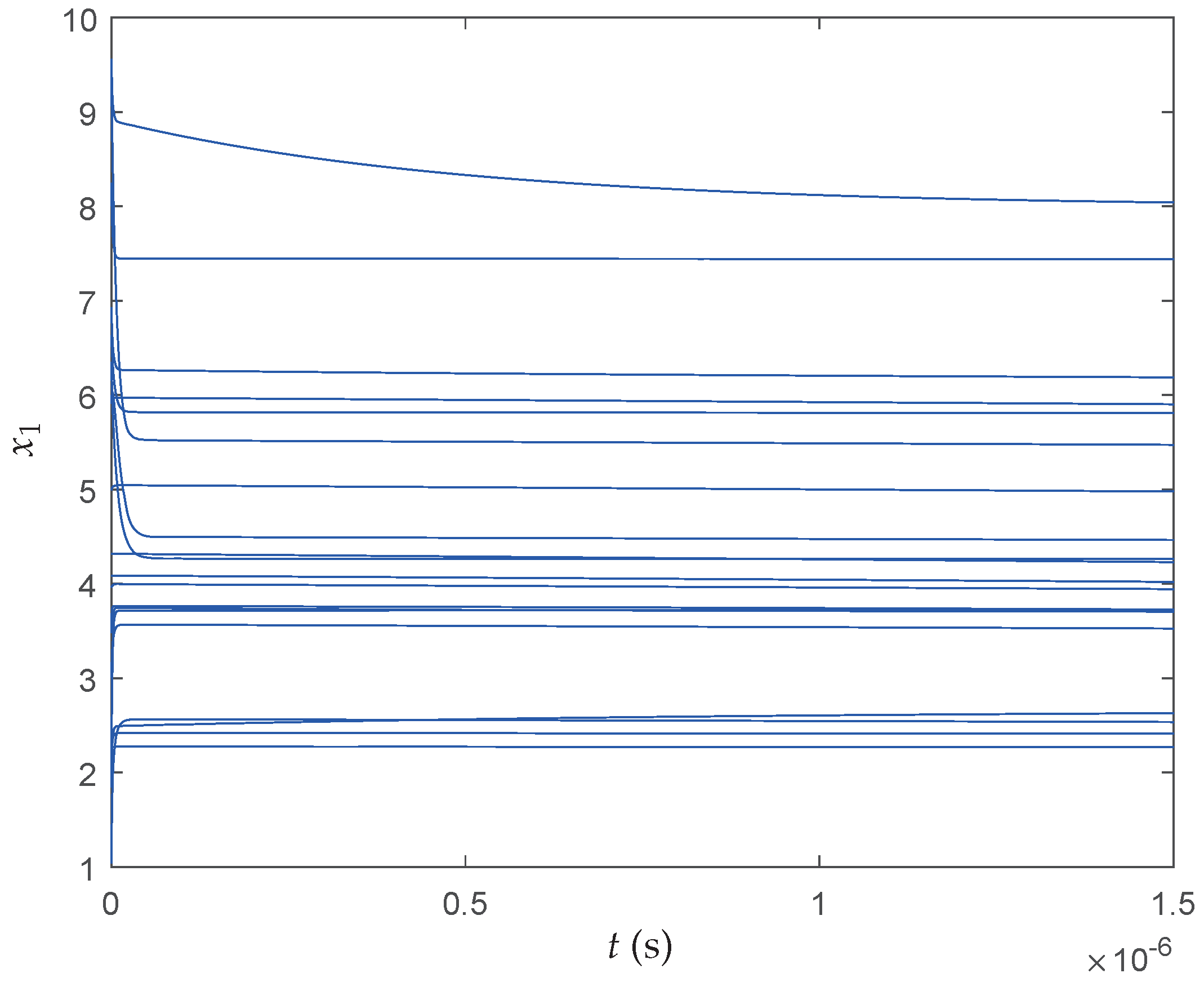
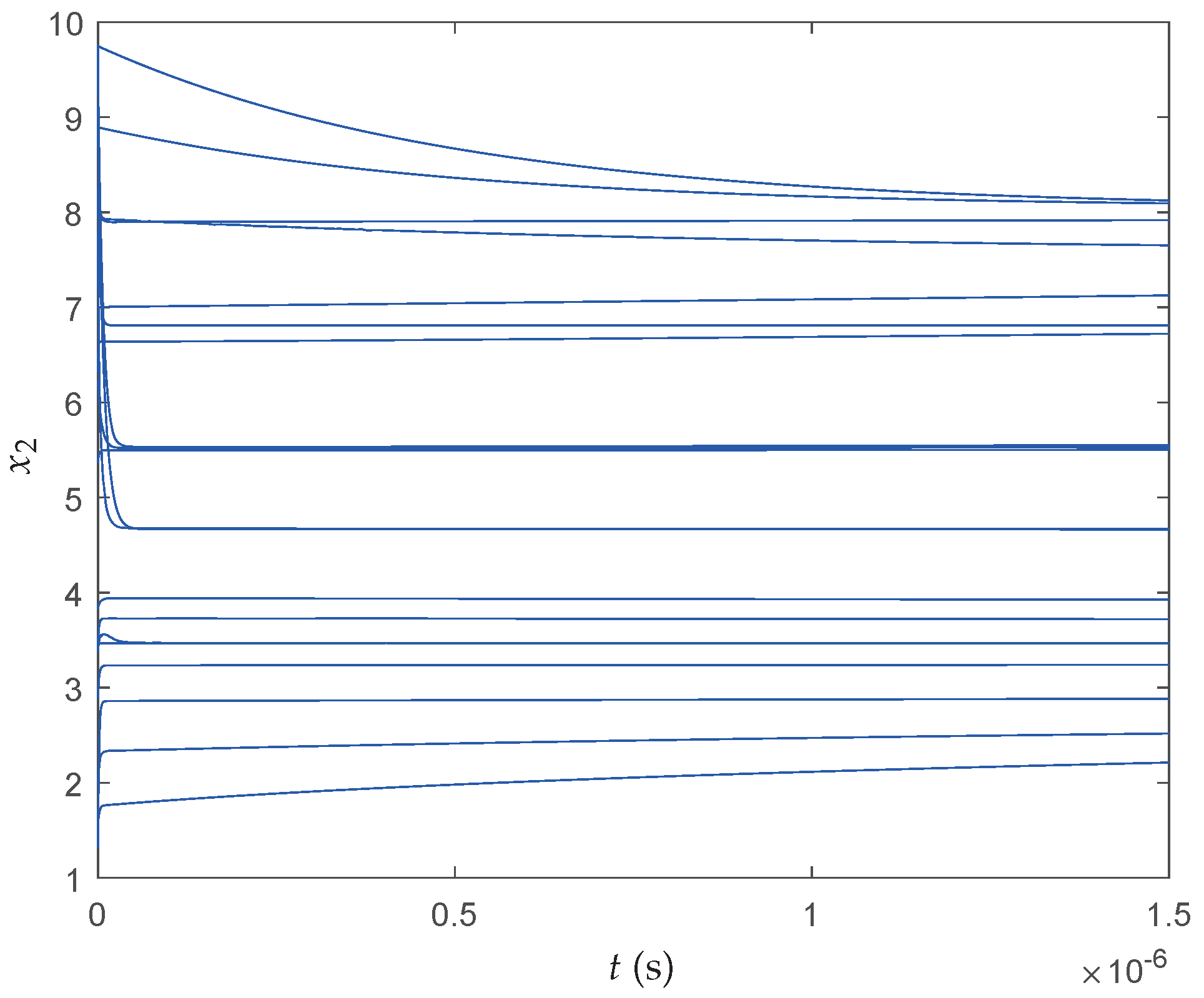
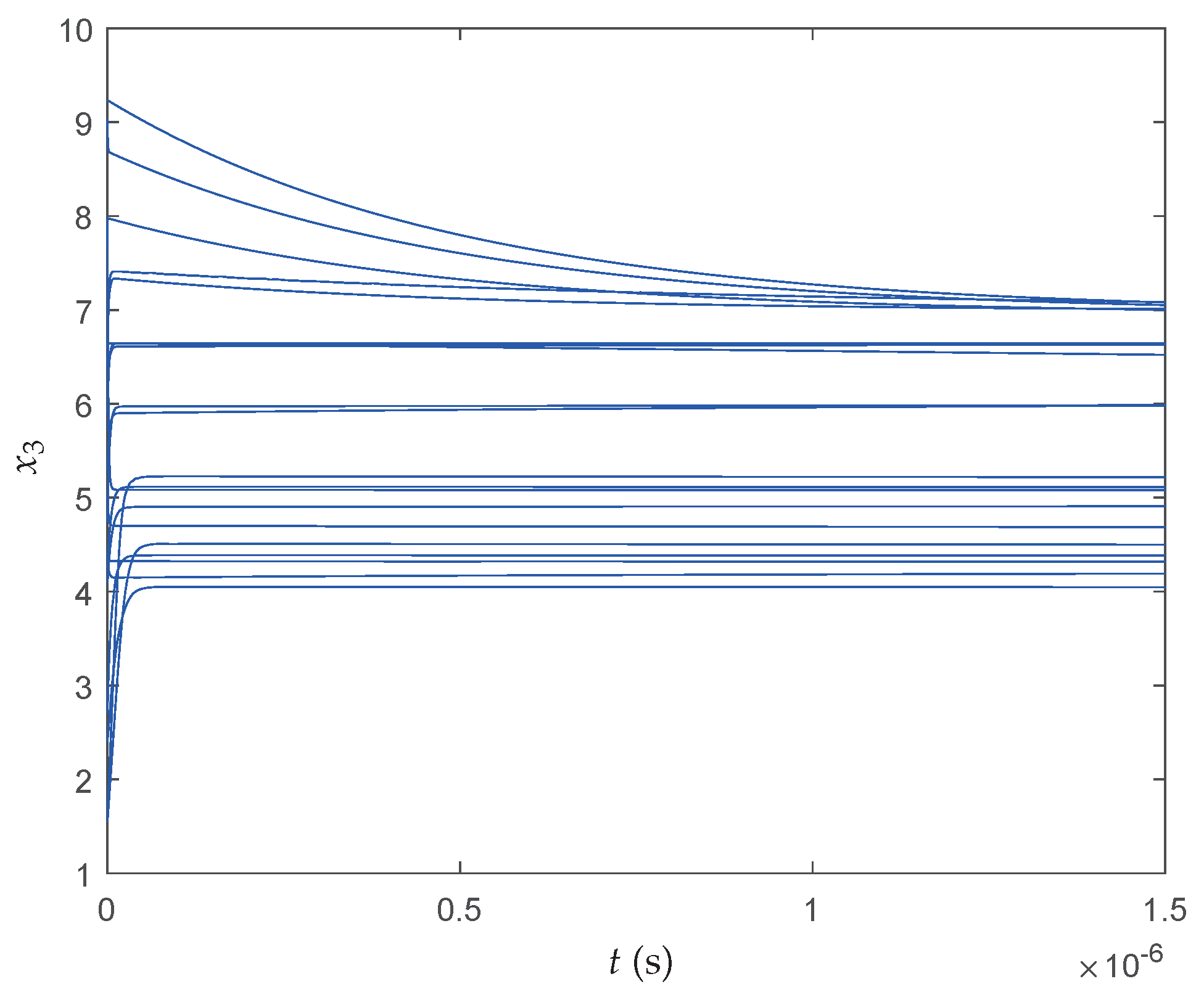
We perform 20 realizations and obtain $x^{\ast }=(5.6691,2.9145,7.0000)$, the minimum cost function value is $0.0050983$, which is better than the result obtained in [36]. Figure 12, Figure 13 and Figure 14 show the transient behaviors of $x_1$, $x_2$ and $x_3$ of the proposed neural network initialized from 20 random particles for each state, respectively. It can be found that all states converge instantaneously local optimal solutions since the cost function itself has many local optima and the searching space is divided into many nonconvex areas by the constraints. Therefore, more iterations have been required to make full use of interconnections of particles so that the QNSO algorithm is able to fully exploit the parallel nature of the computation and produce results that are more globally optimal. Table 6 shows the best result, the average result, the worst result, and the standard deviation result of $f\left(P_g\right)$ over 20 experiments.

Figure 12. Transient behaviors of the proposed neural network state $x_1$.

Figure 13. Transient behaviors of the proposed neural network state $x_2$.

Figure 14. Transient behaviors of the proposed neural network state $x_3$.

Table 6. Statistical analysis of the results in Application 3.

Best	Average	Worst	Std.
$5.0983\times {10}^{-3}$	$5.1364\times {10}^{-3}$	$5.4642\times {10}^{-3}$	$1.1526\times {10}^{-4}$

6. Conclusions

We have presented the design of a new global optimization method called a quantum-behaved neurodynamic swarm optimization (QNSO) approach. This method is composed of an efficient neural network and the quantum-behaved swarm optimization. As the QPSO algorithm is used, the search process in the QNSO method has a high convergence rate. In addition, the global searching ability of particle swarm optimization and the local searching and constraint-processing abilities of neurodynamic optimization can complement each other very well. Meanwhile, the QNSO method and its implementation have been described extensively in the context. Then, the QNSO method has been illustrated with two function tests. Finally, the presented method has been applied to the optimization of three applications.