Free Surface Flow Simulation by a Viscous Numerical Cylindrical Tank

Abstract

In order to numerically investigate the free surface flow evolution in a cylindrical tank, a regular structured grid system in the cylindrical coordinates is usually applied to solve control equations based on the incompressible two-phase flow model. Since the grid spacing in the azimuthal direction is proportionate to the radial distance in a regular structured grid system, very small grid spacing would be obtained in the azimuthal direction and it would require a very small computational time step to satisfy the stability restriction. Moreover, serious mass disequilibrium problems may happen through the convection of the free surface with the Volume of Fluid (VOF) method. Therefore in the present paper, the zonal embedded grid technique was implemented to overcome those problems by gradually adjusting the mesh resolution in different grid blocks. Over the embedded grid system, a finite volume algorithm was developed to solve the Navier–Stokes equations in the three-dimensional cylindrical coordinates. A high-resolution scheme was applied to resolve the free surface between the air and water phases based on the VOF method. Computation of liquid convection under a given velocity field shows that the VOF method implemented with a zonal embedded grid is more advanced in keeping mass continuity than that with regular structured grid system. Furthermore, the proposed model was also applied to simulate the sharp transient evolution of circular dam breaking flow. The simulation results were validated against the commercial software Fluent, which shows a good agreement, and the proposed model does not yield any free surface oscillation.

1. Introduction

The phenomenon of interfacial fluid motions in a cylindrical enclosure, driven by density difference and/or external force, often occurs in technical applications and industrial processes, which will cause a great impact on the working characteristic of the device. That problem arises in applications like liquid sloshing caused by the motion of the cylindrical container. A number of studies have been addressed on those problems. For example, the sloshing behavior in the cylindrical liquid tank has been numerically studied by Hernández-Barrios et al. in [1] and based on the potential theory. In order to simulate the fully nonlinear free surface motions accurately, some recent examples of the computational fluid dynamics (CFD) sloshing simulations have been carried out based on the incompressible two-phase flow model by solving the Navier–Stokes equations and applying appropriate free surface tracking methods, including the studies in [2,3,4,5].

To simulate the flow movement in a cylindrical geometry, the use of the cylindrical coordinate system, if possible, is the most relevant and desirable in the formulation and discretization of the Navier–Stokes equations. For instance, in [6], Fernandez-Feria and Sanmiguel-Rojas developed an incompressible flow simulation model in cylindrical coordinates by an explicit projection method, and He et al. [7] studied the natural convection heat transfer and fluid flow in a vertical cylindrical envelope by a numerical model built in a cylindrical coordinate. However, the resolution of the Navier–Stokes equations in cylindrical coordinates involves some specific difficulties, especially when the computational domain contains the axis r = 0. When the cylindrical center is within the computational domain, terms like $1/r$ or $\partial \varphi /\partial r$ become undefined, which causes a singularity at the cylindrical center. To overcome this problem, many attempts have been made. Ma et al., with a Cartesian mesh in the axis of the cylindrical coordinates, built a numerical model to simulate pipe flow in [8]. 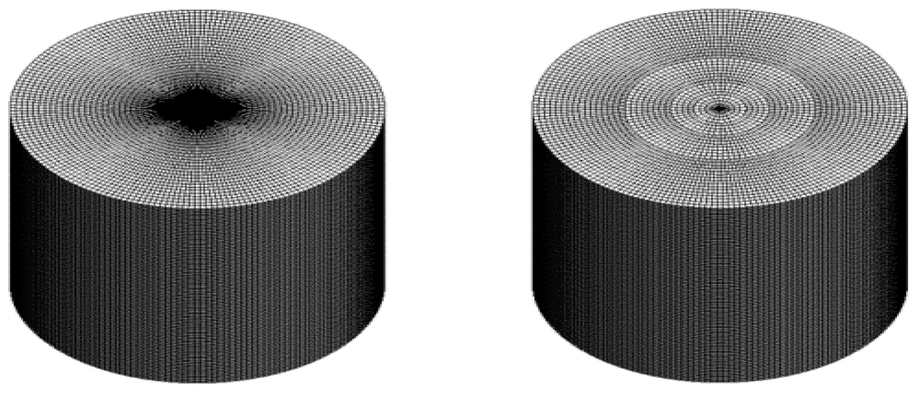In [9], Verzicco and Orlandi avoided this problem by rewriting the Navier–Stokes equations with special variables, which are always zero on the axial, and de Vahl Davis suggested a discretization without nodes on the axis in [10]. Moreover, another problem arises since the mesh size varies with the radial coordinate when the regular orthogonal grid system is applied. Therefore, investigating the flow phenomena within a large-diameter container, the control cells that are far from the origin are much coarser than those that are near the origin, so an extremely small time step should be applied to satisfy the numerical stability. In order to obtain a grid independent solution in cylindrical coordinates, the zonal embedded grid technique, as shown in Figure 1, was implemented in the present paper by locally refining the grid size by blocks, which was originally proposed by Kravchenko et al. in [11] for the accurate computation of a boundary layer above a flat plate, and then developed to a grid system in the two-dimensional polar coordinates in [12] by Suh and Yeo.

Flow simulation performed in the cylindrical coordinates is not new. However, the two-phase incompressible flow model implemented in the cylindrical coordinate system has attracted less attention, and implementing free surface tracking method in the cylindrical coordinates, like the volume of fluid (VOF) method presented in [13], is novel since the surface construction in the VOF method was extremely cumbersome in cylindrical coordinates due to its geometric properties. The VOF method in cylindrical coordinates has been adopted in [14] to analyze the bubble rising problems inside a cylindrical container. In their work, to avoid the complex surface reconstruction process of the VOF method, the interpolated volume fraction at the faces of control volumes was calculated by the first order upwind or downwind scheme according to the free surface orientation. Following this idea, a more accuracy VOF method was proposed in [15] by Ubbink and Issa using the high-resolution based CICSAM scheme (Compressive Interface Capturing Scheme for Arbitrary Mesh) to compute the volume fraction, which could be applied in the cylindrical coordinates.

In the regular mesh system used by Chen et al. in [14], an extremely small time step must be needed to keep the numerical stability, when a bigger computational domain was needed. Thus, the computational results based on that kind of mesh system may lose or acquire volumes when the VOF method is applied, for the unphysical volume that can be ignored in the large control cells may be large enough for that in the smaller control cells. Therefore in this paper, the embedded grid system was adopted to the two-phase flow model in the cylindrical coordinates to acquire a solution independent mesh.

In this paper, the two-phase free surface model was implemented in the cylindrical coordinates within the complex embedded grid system. A finite volume method was used to discretize the Navier–Stokes equations and volume advection equations for the volume fraction over that grid system. To adopt the embedded grid system for the two-phase flow model, special treatment was needed in solving the discretized equations for the Navier–Stokes and fraction advection equations. To validate the advantages of the present model, the VOF method with the embedded grid system was first verified to produce a better mass conservation than that with the regular grid system. Moreover, the sharp transient evolution of 3D circular dam break flow within a cylindrical tank was also presented in this paper, and the simulation results have been validated against the commercial software Fluent.

2. Mathematical Formulation

In this study, the water and air flow movements were considered based on the two-phase incompressible fluid model in a cylindrical computational domain based on the one-fluid assumption. With that assumption, the discontinuous properties through the free surface, such as density and viscosity, are smoothed over a transition region of the finite thickness near the free surface, so the fluid motion of two fluids could be described as the flowing equations:

$$\frac{1}{r}\frac{\partial ru}{\partial r}+\frac{1}{r}\frac{\partial v}{\partial \theta }+\frac{\partial w}{\partial z}=0$$

(1)

$$\begin{array}{cc}\hfill \frac{\partial U}{\partial t}=& -\frac{1}{r}\frac{\partial (ruU)}{\partial r}+\frac{1}{r}\frac{\partial (vU)}{\partial \theta }+\frac{\partial (wU)}{\partial z}\hfill \\ & +\frac{1}{r}\frac{\partial }{\partial r}(\upsilon r\frac{\partial U}{\partial r})+\frac{1}{r}\frac{\partial }{\partial \theta }(\frac{\upsilon }{r}\frac{\partial U}{\partial \theta })+\frac{\partial }{\partial z}(\upsilon \frac{\partial U}{\partial z})+S_U\hfill \end{array}$$

(2a)

$$u:S_U=-\frac{1}{\rho }\frac{\partial P}{\partial r}-\frac{\upsilon }{r}(\frac{2}{r}\frac{\partial v}{\partial \theta }+\frac{u}{r})+\frac{v^2}{r}+\frac{1}{\rho }{f}_{br}$$

(2b)

$$v:S_U=-\frac{1}{\rho }\frac{1}{r}\frac{\partial P}{\partial \theta }+\frac{\upsilon }{r}(\frac{2}{r}\frac{\partial u}{\partial \theta }-\frac{v}{r})-\frac{uv}{r}+\frac{1}{\rho }{f}_{b\theta }$$

(2c)

$$w:S_U=-\frac{1}{\rho }\frac{\partial P}{\partial z}-g+\frac{1}{\rho }{f}_{bz}$$

(2d)

In the above equations, $U=\left(u,v,w\right)$ is the velocity vector; $S_U$ is the source term; $P$ is the pressure; $\rho$ and $\upsilon$ are the density and kinematic viscosity; $F_b=\left(f_{br},f_{b\theta },f_{bz}\right)$ is the vector of the body force due to the surface tension; $t$ is time; and $g$ denotes the gravity acceleration.

The free surface was contracted by the VOF method through marking both fluids with a scalar indictor $F$ defined as the fraction of a control volume occupied by the liquid ($0\ll F\ll 1$). Using the definition of the volume fraction, this work represents the density and viscosity in the momentum equations as

$$\rho =F{\rho }_w+(1-F){\rho }_a$$

(3a)

$$\nu =F{\nu }_w+(1-F){\nu }_a$$

(3b)

where the subscripts $w$ and $a$ denote the water and air fluid. The free surface transport equation in terms of the volume fraction could be written as

$$\frac{\partial F}{\partial t}+\frac{1}{r}\frac{\partial ruF}{\partial r}+\frac{1}{r}\frac{\partial vF}{\partial \theta }+\frac{\partial wF}{\partial z}=0$$

(4)

With the surface normal represented by the gradient of the volume fraction, the unit normal vector for the free surface was given by

$$n=\frac{\nabla F}{\left|\nabla F\right|}$$

(5)

According to the Continuum Surface Force method proposed by Brackbill et al. [16], the smoothed body force used in the momentum equations was given by

$$F_b=\sigma \kappa n\nabla F,$$

(6)

where $\sigma$ and $\kappa$ are the coefficient of surface tension and the curvature of the interface respectively.

3. Numerical Method

3.1. Zonal Embedded Grid

To construct a zonal embedded grid system shown in Figure 1, the method developed by Suh and Yeo in [12] was adopted in the current study. With this method, the entire computational domain was divided into several blocks, and the regular orthogonal grids were generated in each of the blocks, respectively, by refining the grid spacing in the azimuthal direction block by block through the entire computational domain.

3.2. Discretization of the Continuity and Momentum Equations

To solve the control equations, the staggered grid arrangement was applied to store velocities at the cell faces and the scalar variables (pressure, density, viscosity, etc.) at the cell center (Figure 2), and the velocity and pressure field was coupled with the projection method, where an intermediate velocity field $U^{\ast }$ was computed and projected into a divergence-free field with Equations (7a) and (7b), as

$$\begin{array}{cc}\hfill \frac{U^{\ast }-U^n}{\Delta t}=& -\frac{1}{r}\frac{\partial {(ruU)}^n}{\partial r}+\frac{1}{r}\frac{\partial {(vU)}^n}{\partial \theta }+\frac{\partial {(wU)}^n}{\partial z}\hfill \\ & +\frac{1}{r}\frac{\partial }{\partial r}{(\upsilon r\frac{\partial U}{\partial r})}^n+\frac{1}{r}\frac{\partial }{\partial \theta }{(\frac{\upsilon }{r}\frac{\partial U}{\partial \theta })}^n+\frac{\partial }{\partial z}{(\upsilon \frac{\partial U}{\partial z})}^n+S_U^n\hfill \end{array}$$

(7a)

$$U^{n+1}=U^{\ast }-\frac{\Delta t}{{\rho }^{n+1}}\nabla (P^{n+1}-P^n)\stackrel{P^{\prime }=P^{n+1}-P^n}{\to }\nabla ·U^{\ast }=\Delta t\nabla ·\frac{1}{{\rho }^{n+1}}\nabla P^{\prime }$$

(7b)

where $n$ and $n+1$ donate the previous and new time layers. The intermediate velocity could be computed by discretizing the convection, diffusion and source terms in Equation (3a) over the control volumes by using the finite volume method. For the orthogonal grids, by integrating the convection term over the control volumes, it yielded

$${\displaystyle \int (\frac{1}{r}\frac{\partial (ruU)}{\partial r}+\frac{1}{r}\frac{\partial (vU)}{\partial \theta }+\frac{\partial (wU)}{\partial z}})\mathrm{d}V={\displaystyle \int U_{f}U·n_f\mathrm{d}A}$$

(8)

in which $n_f$ is the unit surface vector of cell faces and $U_f$ is the velocity at the cell faces of the control volume, which could be determined by a high-resolution scheme as the Sharp and Monotonic Algorithm for Realistic Transport (SMART) scheme by Gaskell and Lau in [17].

Integrating the diffusion term in Equation (7a) over the control volume, it was given as

$${\displaystyle \int (\frac{1}{r}\frac{\partial }{\partial r}(\upsilon r\frac{\partial U}{\partial r})+\frac{1}{r}\frac{\partial }{\partial \theta }(\frac{\upsilon }{r}\frac{\partial U}{\partial \theta })+\frac{\partial }{\partial z}(\upsilon \frac{\partial U}{\partial z})})\mathrm{d}V={\displaystyle \int \upsilon \nabla U_f·n_f\mathrm{d}A},$$

(9)

where the gradient of the velocity at the faces of control volume was computed by the central difference scheme. The source term in Equation (7a) was assumed to be piecewise uniform over each volume, discretized as

$${\displaystyle \int S_U\mathrm{d}V=}{S}_U\Delta V$$

(10)

By invoking the Green’s theorem, Equation (7b) could be written as

$${\displaystyle \int U^{\ast }·n_f\mathrm{d}A}=\frac{\Delta t}{{\rho }^n}{\displaystyle \int \nabla P^{\prime }·n_f\mathrm{d}A}$$

(11)

where $\nabla P^{\prime }$ or $\nabla P$ at the normal faces is evaluated with a central difference scheme, and special concerns should be paid in the treatment of $\nabla P^{\prime }$ or $\nabla P$ at the interface between two blocks. Losasso et al. simulated a two-phase flow motion over an adaptive octree grids system in the three-dimensional Cartesian Coordinates by treating the gradient at the interface to be interpolated over cells that shared the same faces in [18], and the interpolation scheme used in that study was introduced to the present algorithm. Therefore, the pressure gradient at the west faces of the control cells $EN$ and $ES$ shown in Figure 2b should be kept the same, which could be formulated as

$${\frac{\partial P}{\partial r}}_{ES}={\frac{\partial P}{\partial r}}_{EN}=\frac{(P_{ES}+P_{ES})-2P_P}{2\Delta r}$$

(12)

This interpolation yields a symmetric coefficient matrix for the pressure, which enables the use of the iterative solver, such as the preconditioned conjugate gradient (PCG) method. In this paper, the pressure Poisson equation was solved by using an algebraic multi-grid method (AMG).

3.3. VOF Method

As the volume fraction used in the VOF method is a step function, the problem arises of how to advect without numerical diffusing, dispersing or wrinkling accompanying with its convection across a mesh. To avoid those problems, various VOF methods that can be categorized as Lagrangian and algebraic methods have been proposed. With the Lagrangian methods, the free surface should be firstly rebuilt at each computational time step based on the volume fraction with the interface reconstruction methods, like the SLIC method (Simple Line Interface Calculation, presented by Noh and Woodward in [19]) and the PLIC method. Then, the reconstructed surface was advected explicitly. With the algebraic methods, such as the Thinc method reported in [20], the Flux-Corrected Transport method presented in [21] and the CICSAM method, the high order convection schemes and mathmatical limitor was used to constrain the flux across the cell faces. To avoid that complexity, algebraic methods are more suitable methods to track the free surface in the cylindrical coordinates.

In order to solve the VOF convection equation, the CICSAM method based on the donor and acceptor method in the original VOF method by Hirt and Nichols in [13], and the high-resolution scheme was applied in this work. In the CICSAM method, volume fraction was first approximated with the implicit Crank–Nicholson method, and then an iterative correction procedure was applied to correct the unphysical values. To simplify the computation, Heyns et al. implemented a Jacobi type dual-time stepping formulation approach in [22] by reformulating the original VOF convection equation as

$$\frac{F^{\tau +1}-F^{\tau }}{\Delta \tau }+\frac{F^{\tau }-F^n}{\Delta t}=-\frac{1}{2}(\frac{1}{r}{\frac{\partial ruF}{\partial r}}^{\tau }+\frac{1}{r}{\frac{\partial vF}{\partial \theta }}^{\tau }+{\frac{\partial wF}{\partial z}}^{\tau }+\frac{1}{r}{\frac{\partial ruF}{\partial r}}^n+\frac{1}{r}{\frac{\partial vF}{\partial \theta }}^n+{\frac{\partial wF}{\partial z}}^n)$$

(13)

by approaching the implicit solution with an explicit method as it converges in the pseudo time $\tau$. With the finite volume method, the discretized form of Equation (13) could be written as:

$$\frac{F^{\tau +1}-F^{\tau }}{\Delta \tau }+\frac{F^{\tau }-F^n}{\Delta t}=-\frac{1}{2}\frac{1}{\Delta V}{\displaystyle \int (F_f^{\tau }+F_f^n)U^{n+1}·n_f\mathrm{d}A}$$

(14)

where $F_f^{\tau }$ and $F_f^n$ are volume fractions defined at the faces of the control cell, which can be calculated by the CICSAM scheme, and $\Delta \tau$ is the pseudo time step set to be $2\Delta t/3$.

To avoid numerical oscillations at the interfaces between two blocks, the flux-constraint technique used in the velocity computation was adopted to keep the flux of the volume fraction the same in this study.

3.4. Treatment at Origin

In the present model, no velocity was defined at the origin, so the mathematical singularity could be avoided by adopting the staggered grid arrangement on the discretization of the governing equations.

3.5. Solution Procedure

At each time step, the intermediate velocity was computed from Equation (7a) using the variables at the previous step, and the correction pressure was then solved using the pressure Poisson equation (Equation (7b)). Then, the velocity and pressure were iteratively updated using the correction pressure computed by Equation (7b) until the conservation law was fulfilled. After the velocity was calculated, VOF method was used with Equation (13) to advect the water and air interface.

4. Results and Discussions

The numerical algorithms proposed in this study were implemented to the simulate the free surface motions in a three-dimensional circular tank. In order to demonstrate the advantage of the embedded grid technique in the cylindrical coordinates, movements of a volume of fluid were simulated under a given velocity, and comparison of the volume loss with that using the regular grids was also presented. Moreover, the present two-phase flow model was applied to compute sharp transient evolution of the circular dam break flow, which was validated against the simulation results predicted by Fluent.

4.1. Validation of the VOF Method with the Zonal-Embedded Method

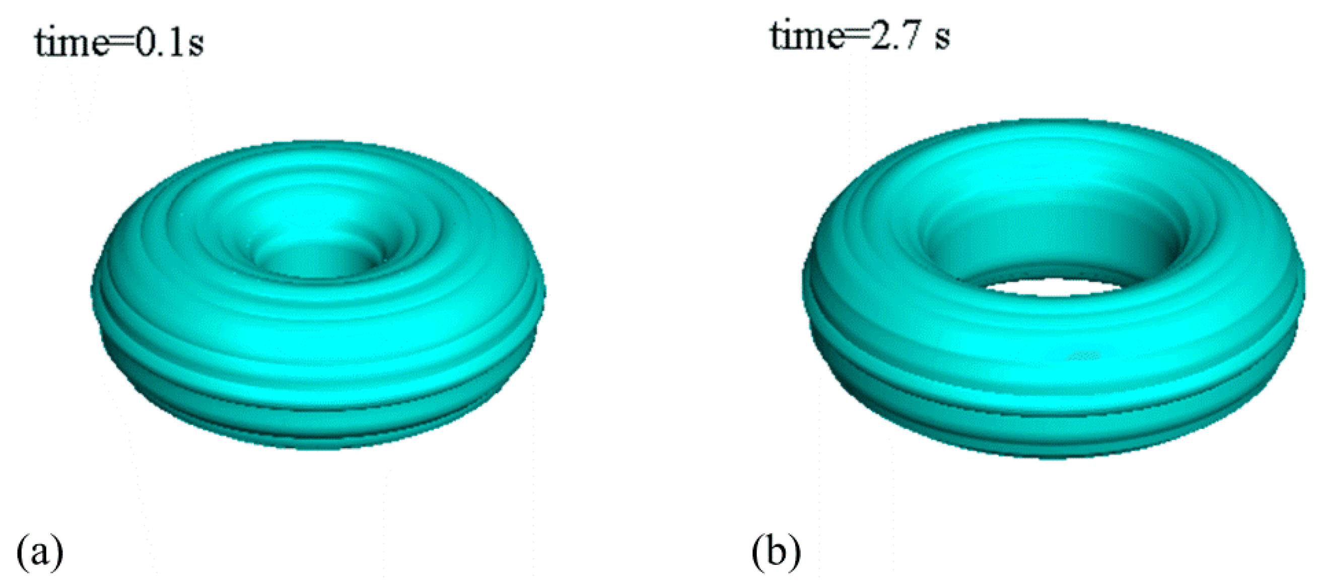
To outline the effect of the embedded grid system on the VOF method, the simulation of an axisymmetric O ring (the inside diameter of it is 0.4 m and the width is 0.6 m) moving with a velocity field $U=\left(0.01/r,0,0\right)$ was carried out. The whole computational domain was divided into four blocks, and the mesh sizes in these blocks are $4\times 25\times 100$, $4\times 50\times 100$, $8\times 100\times 100$. and $16\times 200\times 100$ in the $r$, $\theta$ and $z$ coordinates. That case was also computed as a comparison using the regular orthogonal grid with mesh sizes of $32\times 200\times 100$.

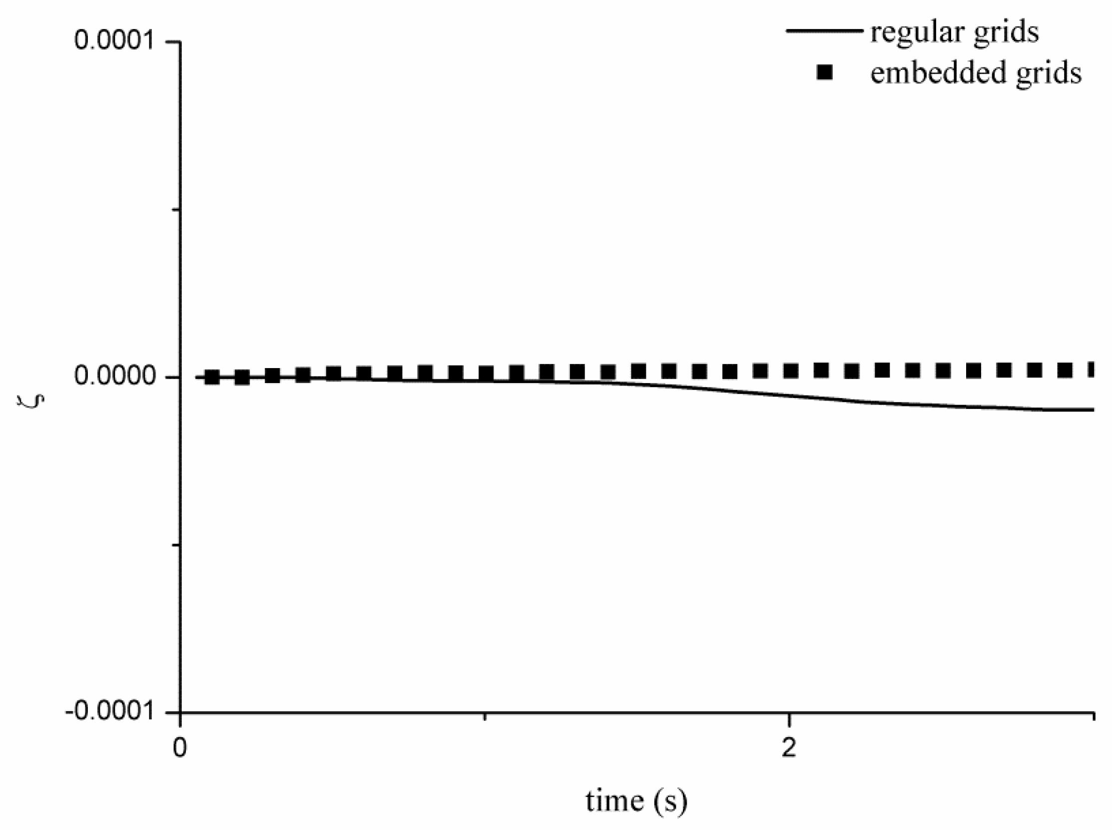
Figure 3 shows the three-dimensional snapshots of the O ring with the embedded grid system. Results from the VOF method with the zonal embedded grid system are superior to the results of that with the regular grid due to the mass disequilibrium. A better continuity property can be obtained with the zonal embedded grid system as shown in Figure 4. In this figure, the ratio of the mass loss is defined by

$$\zeta =\frac{V_{In}-V_t}{V_{In}}$$

(15)

where $V_t$ and $V_{in}$ are the instantaneous and initial volume of the O ring.

4.2. Breaking of the Circular Dam

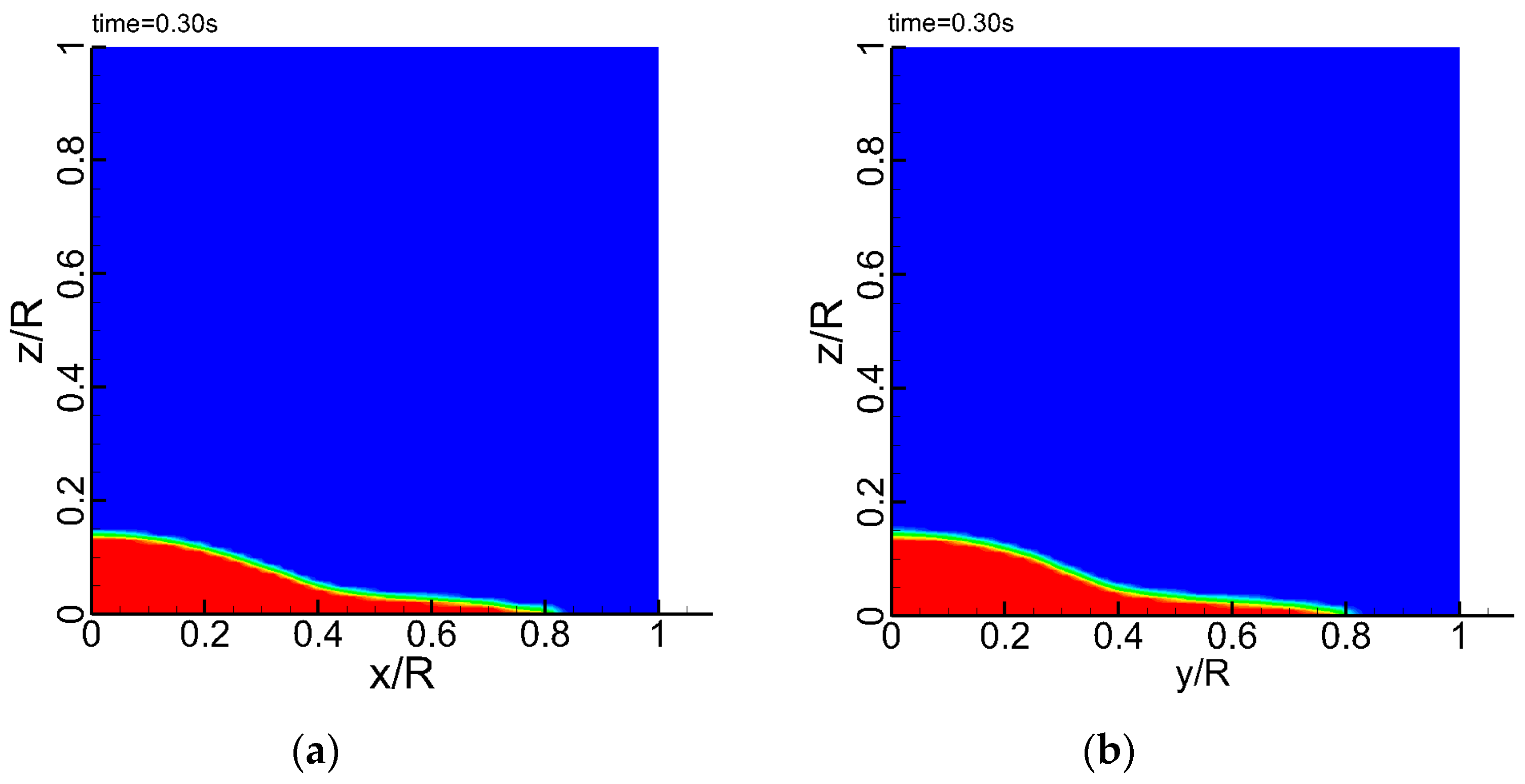
The numerical method was also validated in the performance of the VOF method against a circular dam-break problem. This problem is essentially two-dimensional in the radial and vertical directions. Hence, this provides a possibility to check the ability of the method to preserve symmetry in the numerical solution since the special treatments for the zonal embedded grid system are applied along the radial direction.

Circular dam-break problems are normally used to test the capability of models for the symmetric free surface simulations. It was studied by Zoppou and Roberts in [23] with a shallow water equation solver and Lin et al. in [24] also applied it to validate their component-wise TVD scheme for the shallow water equations. In this paper, a cylindrical column of water of diameter 0.6 m and height 0.3 m initially at rest is allowed to collapse instantaneously under gravity at the center of the circular tank. The computational mesh size in every block was $5\times 20\times 60$, $5\times 40\times 60$, $10\times 80\times 60$, $20\times 160\times 60$ and $20\times 320\times 60,$ and uniform grid spacing of $\Delta r=\Delta z=0.02\mathrm{m}$ was used in both the radial and vertical direction. The snapshots of water depth distributions are represented in Figure 5 and Figure 6 for t = 0.15 s and 0.3 s. They show that the results obtained with the zonal embedded grid system could maintain the cylindrical symmetry of the exact solution and reserve the bore wave without oscillations. Comparisons of the numerical results with that computed by the commercial software Fluent have been demonstrated successively in Figure 5, Figure 6, Figure 7 and Figure 8, and it can be seen that the nearly same distribution of the free surface is obtained using the current model and the Fluent software.

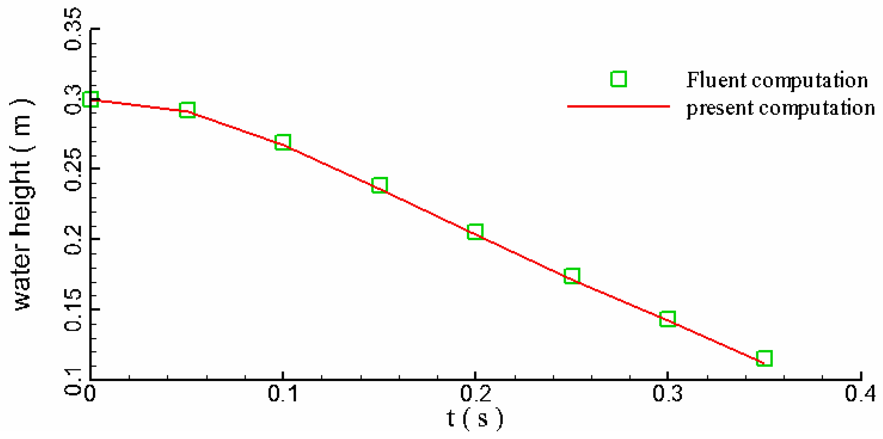
In order to illustrate the results more clearly, the temporal evolutions of water depth and the front position of the dam break flow have been plotted in Figure 9 and Figure 10, respectively, which show the predictions by current model are in good agreement with that computed by Fluent, indicating that the current model could simulate the free surface movements in a cylindrical water tank with an acceptable accuracy.

5. Conclusions

A numerical method was constructed to study the flow motion inside a cylindrical tank with the VOF method to resolve the free surface in cylindrical coordinates. In order to obtain a grid independent solution within a large-diameter computer domain, the zonal-embedded grid method was also adopted to adjust the grid resolution gradually in the radial direction. Special treatments for the embedded grids in discretizing the Navier–Stokes and VOF convection equations were presented in detail.

The VOF method was checked with the case of liquid convection under a given velocity field, and better results were obtained with the zonal embedded method in the mass conservation property. Then, the algorithms were validated against the circular dam breaking problem. Reasonable agreement has been demonstrated by comparing the numerical results with simulation data computed by Fluent. Through those results, it is demonstrated that the presented numerical model can reliably simulate the interfacial flow motions in a circular tank. Moreover, the study on water sloshing in a cylindrical water tank will be our future work in order to develop this model in engineering applications.