Article

Optical Flow Estimation with Occlusion Detection

1
Institute of Intelligent Machines, Chinese Academy of Sciences, Hefei 230031, China
2
Department of Automation, University of Science and Technology of China, Hefei 230026, China
*
Author to whom correspondence should be addressed.
Algorithms 2019, 12(5), 92; https://doi.org/10.3390/a12050092
Submission received: 19 March 2019 / Revised: 23 April 2019 / Accepted: 23 April 2019 / Published: 1 May 2019

Abstract

:
The dense optical flow estimation under occlusion is a challenging task. Occlusion may result in ambiguity in optical flow estimation, while accurate occlusion detection can reduce the error. In this paper, we propose a robust optical flow estimation algorithm with reliable occlusion detection. Firstly, the occlusion areas in successive video frames are detected by integrating various information from multiple sources including feature matching, motion edges, warped images and occlusion consistency. Then optimization function with occlusion coefficient and selective region smoothing are used to obtain the optical flow estimation of the non-occlusion areas and occlusion areas respectively. Experimental results show that the algorithm proposed in this paper is an effective algorithm for dense optical flow estimation.

1. Introduction

The concept of optical flow, describing the apparent motion between images or video frames, arises from the studies of biological visual systems. In certain applications, it is desirable to identify optical flow everywhere in the whole image, such as video segmentation [1], three-dimensional reconstruction [2], and video compression [3]. Occlusion destroys the consistency constraint in optical flow estimation, for example, the assumption that the pixel characteristics are unchanged before and after motion. In addition, the consistency constraint may cause unavoidable errors in the occlusion areas. Therefore, correctly distinguishing the two areas and using different optimization strategies can improve the accuracy of optical flow estimation.
The methods of optical flow estimation can be roughly divided into three categories: the variational methods [4], the matching methods [5] and the approximate nearest neighbor fields (ANNF) methods [6]. In addition to the above three methods and the mutual integration [7], the Convolutional Neural Network (CNN)-based methods are obtaining considerable attention in recent years. Flownet [8], Flownet2.0 [9] and SPyNet [10] are all the end-to-end convolutional architectures. DM-CNN [11], MC-CNN [12], PatchBatch [13] and many others CNN-based methods are of matching-based architectures. Besides Sevilla-Lara et al. [14], Bai et al. [15] and Shen et al. [16] apply segmentation results to assist optical flow estimation. However, most of the above methods do not deal with occlusion directly, instead they treat them as the outliers and suppress the influence of occlusion by introducing complex penalty terms, such as the Lorentzian potentials [17] and the Charbonnier potentials [18]. This is the compromise using the consistency constraints in the whole image. For the occlusion area, this is the wrong optimization function, so it will lead to the undesirable results. Because it is a global optimization function, ambiguity may even affect the optical flow in the non-occluded areas. Owing to the lack of feature information in the occluded areas, the smoothing term is often used to deduce the optical flow in the occluded area, but it results in over-smoothing optical flow. The image-adaptive, isotropic diffusion [19], anisotropic diffusion [20], and isotropic diffusion with non-quadratic regularizes [17] are proposed to deal with over-smoothing, but they do not account for occlusions. Hur et al. [21] proposed the jointly estimate disparity and occlusions method, but its huge computation cost is intolerable in most applications. Therefore, in practice, a three-step-approach [22] is proposed, with the occlusion-unaware optical flow firstly estimated, then the occlusion areas identified and finally the optical flow corrected.
Complex penalty terms cannot fundamentally eliminate the influence of occlusion. Bidirectional optical flows in joint optimization would result in huge computational redundancy. In addition, the three-step-approach relies heavily on the quality of occlusion detection. Therefore, in this paper, we propose a more robust optical flow algorithm with occlusion detection, and the overall flow of the proposed method is shown in Figure 1. The contributions of this proposed research include two aspects.
For occlusion detection, we mine occlusion information from multiple directions, and propose a regional-based fusion strategy. Matching can provide the most basic occlusion detection results, which do not depend on optical flow. However, because it often only uses the simple features, it may appear false positive phenomenon, which may be invalid in edge areas or illumination changes. Warped image is the intermediate result of the coarse to fine warping algorithm, from which we found the trace of occlusion creatively. Through motion analysis, we find that the ghosting artifacts are the occlusion areas, but this method depends on the quality of optical flow estimation. The occlusion only appears on the moving edges, and the moving edges of the two images surround the candidate area of occlusion. We fuse the above three kinds of information into an initial occlusion detection result. Because occlusion has regional consistency, we propose a regional-based optimization strategy. Since the occluded edge is composed of the moving edges of two images, we first fuse the two images, and then optimize the occlusion detection results by using the regional consistency.
For optical flow estimation, we use two optimization strategies for different areas. Using the occlusion detection results obtained from the above work, the whole image is divided into occlusion areas and non-occlusion areas. We use a modified energy function for non-occlusion area. Due to the lack of effective information, neighborhood smoothing are often used for optical flow in the occlusion areas. Based on the discrimination of occlusion and non-occlusion areas, we not only improve the efficiency and accuracy of the optimization function, but also reduce the influence of smoothing operation on the results, thus obtaining better optical flow estimation results.
The remainder of this paper is organized as follows. We discuss the related work in Section 2. Our occlusion detection strategy are given in Section 3. Our occlusion-aware optical flow estimation are given in Section 4. Experimental results and analyses are presented in Section 5. Our conclusion and future work are summarized in Section 6.

2. Related Work

Most optical flow approaches are based on a variational formulation since it can obtain sub-pixel level results naturally. Occlusion phenomena are ubiquitous in optical flow estimation, and there is abundant literature on this topic. In this section, we briefly review the variational methods and the occlusion-aware optical flow estimation.
Following the variational model of Horn and Schunck [23], modern optical flow estimation is usually posed as an energy minimization problem, which includes an energy function containing a brightness constancy assumption and a smoothness assumption. Hierarchical (pyramid-based) algorithms have a long history [24], and it is widely used in optical flow estimation presently, such as S2F [25] and MirrowFlow [21]. Hierarchical algorithms first estimate the optical flow on smaller, lower-resolution images and then use them to initialize higher-resolution estimates. The advantages of which include increased computation efficiency and with the ability to find better solutions (escape from local minima). Weickert et al. [26] systematically summarized the previous work on the data term and the smoothing term. Monzon et al. [27] did further work on the selection of the smoothing terms, and they found that the automatic setup of decreasing scalar functions(DF-Auto) for regularization can achieve a good balance between robustness and accuracy. LDOF [7] creatively integrated the histograms of oriented gradients (HOG) descriptors into the coarse-to-fine warping methods, and achieved the remarkable results. A quantitative analysis of optical flow estimation was proposed by Sun et al. [28], and they verified that the importance of the median filtering.
Occluded pixels have undefined flow, so that good estimation of flow depends on occlusion and vice versa. Based on the methodology, we divide them into three major categories. The first category treats occlusion as outliers and suppresses the influence of occlusion by complex penalty terms, the L1-norm potentials were introduced by Brox [29] and have been widely used by many other researchers due to its robustness. Motivated by the statistics of optical flow, the Lorentzian potentials and the Charbonnier potentials are proposed successively. The second category deals with occlusion by exploiting the symmetric property of optical flow and analyzing the bidirectional optical flow. Alvarez et al. [30] proposed one such solution, computing symmetrically dense optical flow which is consistent from frame 1 to frame 2 and frame 2 to frame 1. This is achieved by minimizing an energy function which respects occlusion. The last category builds more sophisticated frameworks to reasoning occlusion. Kennedy et al. [31] proposed a triangulation-based framework using a geometric model that can directly account for occlusion effects. FullFlow [32] optimized a classical optical flow objective over the full space of mappings between discrete grids, which can deal with occlusion simultaneously. MR-Flow [33] proposed a deep learning framework for rigid region reasoning, which makes use of its integrity to circumvent the occlusion detection process.

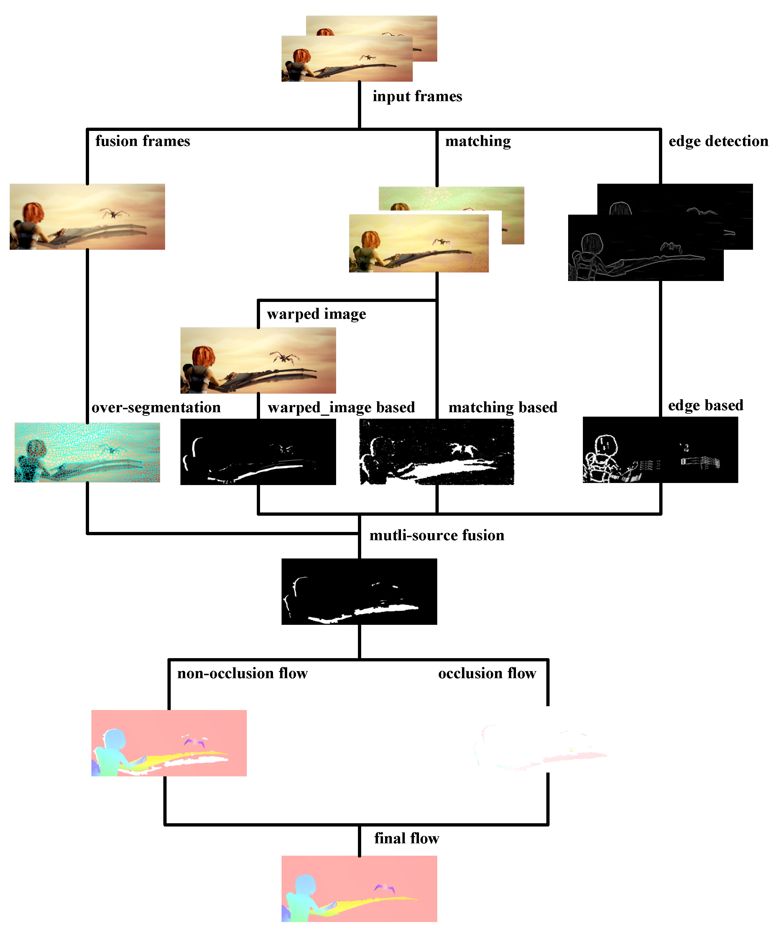
3. Occlusion Detection Strategy

The three-step optical flow estimation depends heavily on the quality of occlusion detection, so reliable occlusion detection results are very important for optical flow estimation. In this section, we will propose our occlusion detection strategies based on various information, and our fusion strategy will be proposed in the last subsection.

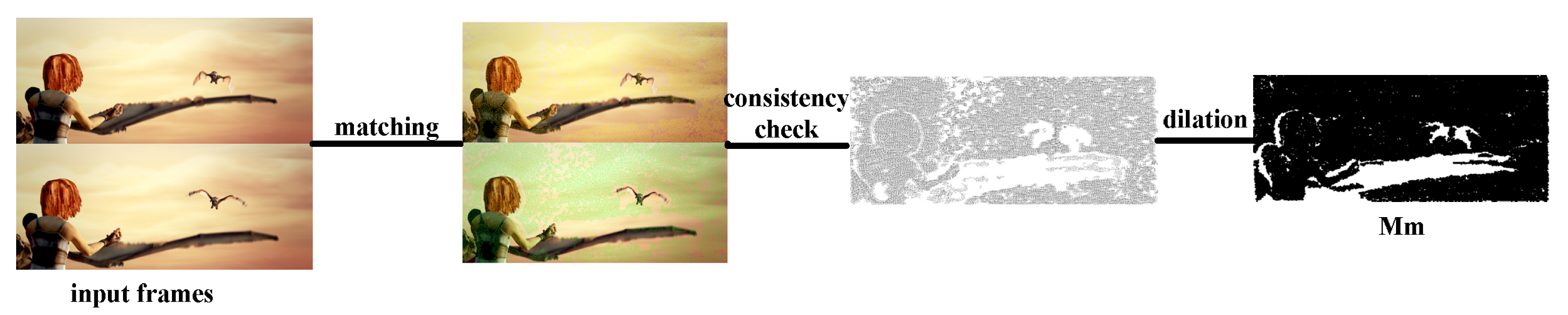
3.1. Matching-Based Strategy

Optical flow estimation can be considered as a matching problem. Comparing two frames of images, occlusion can be determined if a pixel does not appear in the second frame. We can use either color features or more complex features for matching. In order to balance computation cost and computational accuracy, we do not match point-by-point, but use grid point sampling algorithm. To be specific, we first generate grids with a fixed size of 5 in both frames. For each sampling point, we build two descriptors H and C and use these descriptors for matching. H consists of 9 orientation histograms with 12 bins and C comprises the mean RGB color of 9 subparts. Correspondences between points are obtained by approximate K-nearest neighbor matching, which K is 2 in our strategy. We compute the Euclidean distances of both descriptors separately and normalize them by the sum over all distances.
d 2 ( H m , H n ) = H m H n 2 2 1 S i , j H i H j 2 2
d 2 ( C m , C n ) = C m C n 2 2 1 S i , j C i C j 2 2
d 2 ( m , n ) = 1 2 ( d 2 ( H m , H n ) + d 2 ( C m , C n ) )
where m is the grid points in the first frame and n is the matched point in the second frame, S is the total number of combinations m, n. Due to the normalization, H and C share the same weight in the final distance. The next step is consistency check, which is helpful for removing outliers. Since the matching results are sparse, we need sparse-to-dense interpolation to obtain the initial occlusion detection M m , and the overall flow of our matching-based strategy is shown in Figure 2.
We also experimented with the KD-tree-based matching algorithm proposed by He et al. [34] and the Siamese neural network based matching methods [35]. The former algorithm achieves similar results of the above one, but its computational complexity is greater. Perhaps due to the lack of sufficient training data, the CNN-based algorithm has not achieved satisfactory results.

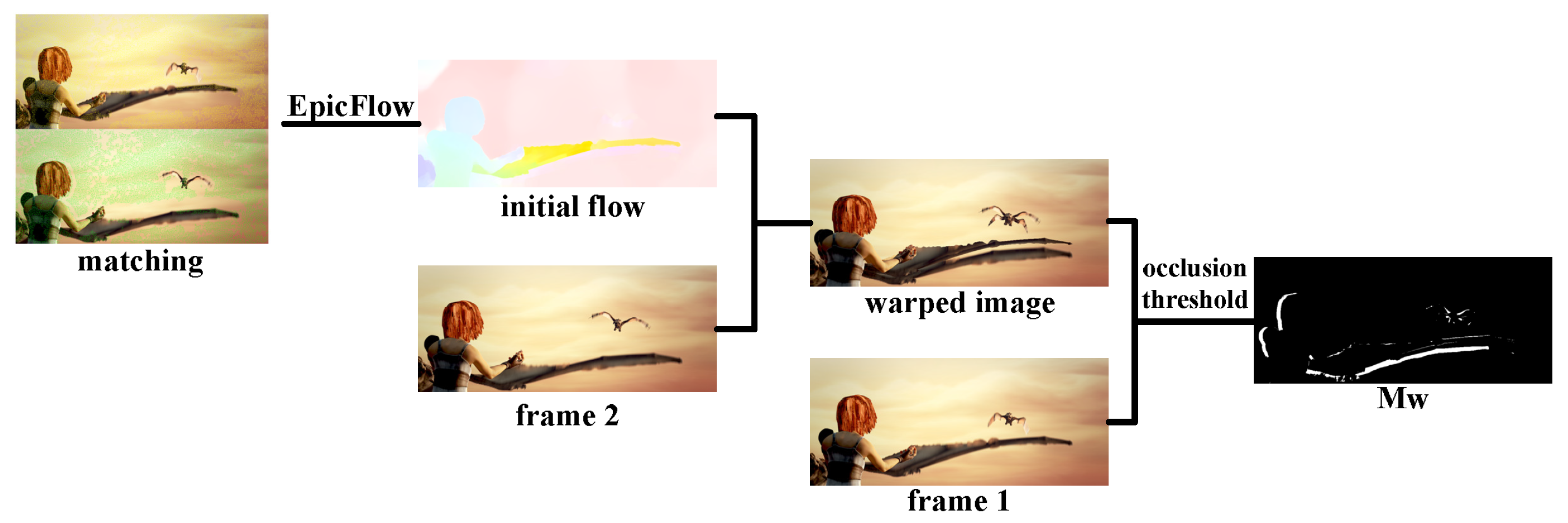
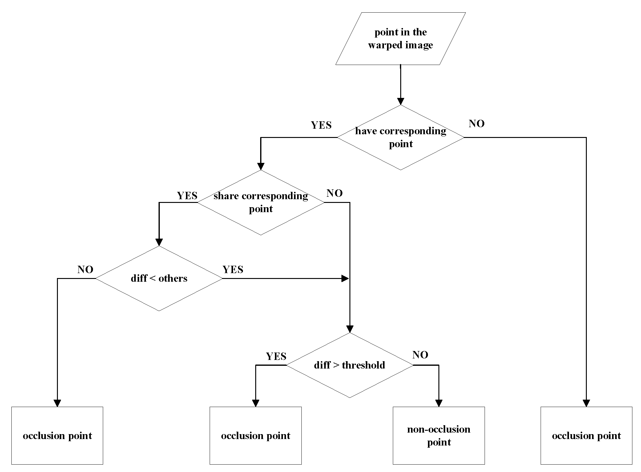
3.2. Warped Image-Based Strategy

Using the initial matching mentioned above and EpicFlow [36], the initial optical flow estimation can be estimated, which contains abundant occlusion information. We get the occlusion reasoning from two aspects, one is the motion analysis, and the other is warped image. The overall flow of our matching-based strategy is shown in Figure 3.
Based on the statistics [9] of Flying Chairs and the MPI-Sintel datasets, it is verified that the displacements of the foreground are larger than that in the background. Meanwhile, the occluded areas belong to the background in most cases. According to the transformation matrix from optical flow, if more than one pixels move to the same position, the positions with small optical flow values are marked as occlusion. Based on the above motion analysis, we can obtain occlusion detection results to some extent. Meanwhile, the warped image also contains abundant occlusion information. Under the guidance of optical flow, the warped image can be obtained by backward mapping of frame 2. Occlusion might result in undesirable ghosting artifacts in the warped image which is helpful for reasoning occlusion.
The above two strategies can get occlusion detection separately. Since the statistical results are not applicable to each frame, the former strategy method may lead to many errors. In addition, the latter is sensitive to the threshold of the difference. Therefore, we propose a robust and reliable combined detection strategy, which is shown in Figure 4 and the initial occlusion detection is named as M w . According to the motion analysis, the positions in the first frame are divided into three categories. The first category is that there is no corresponding point in frame 2. A unique corresponding point in frame 2 is the second category. In addition, the last category is sharing the corresponding point in frame 2 with other positions. For “many to one” relationship in the third category, we only retain the smallest difference correspondence. No corresponding relationship can be directly reasoned as occlusion. In the “one to one” relationship, occlusion threshold is used to determine whether there is occlusion. Since the pixels in the warped image are obtained by neighborhood interpolation, the occlusion threshold can be designed to correlate with the maximum difference of the pixels in the four neighborhoods.

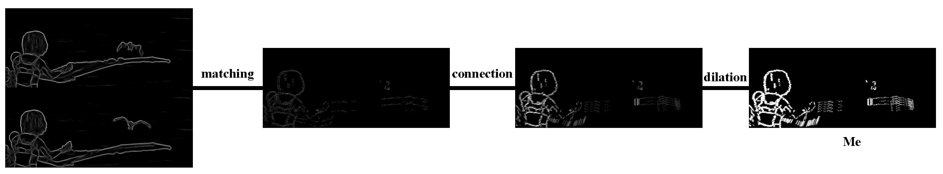
3.3. Edge-Based Strategy

Since occlusion is caused by movement, so it would appear on the moving edges. The moving edge is the complex semantic information, so usually using image edge to approximate. By connecting the matching edges of two frames, we can obtain the occlusion candidate M e . The overall flow of our edge-based strategy is shown in Figure 5.
Firstly, we calculate the edges of two frames using a recent state-of-the-art edge detector, namely the “structured edge detector” (SED) [37]. Then we use the descriptor matching algorithm mentioned above to calculate the matching relationships in the edge areas. By interpolating the retained matching points, we can get the occlusion candidate areas at image edge areas.

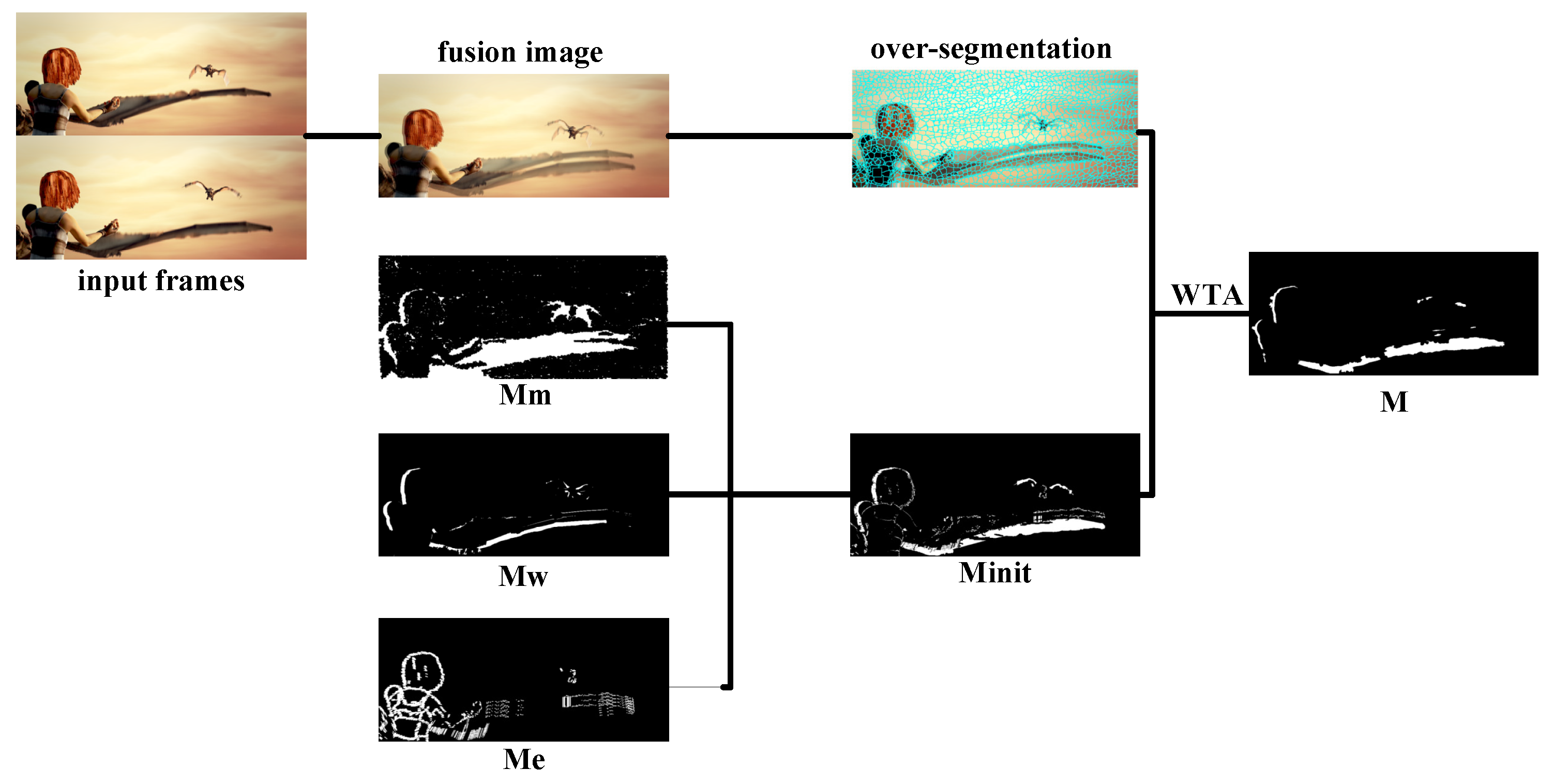
3.4. Regional-Based Fusion Algorithm

Integrating the above occlusion detection results based on edges at first since the M e is meaningless in non-edge areas and the M w is applied to a more relaxed threshold in edge areas.
M i n i t = α M m + β M w + γ M e α , β , γ > 0 α + β + γ = 1
where α , β and γ are tuning parameters which can be determined manually according to qualitative evidence on datasets, or be estimated automatically from ground truth data. Through the subsequent experiments, we fixed all parameters at [0.3, 0.3, 0.4] in the edge areas, and [0.4, 0.5, 0.1] in the non-edge areas.
Since the motion has regional consistency, neighborhood information is helpful for occlusion reasoning. The consistent regions in a single frame is not enough for occlusion reasoning because occlusion appears on the moving edges. Firstly we overlay two frames, and then we obtain the consistent regions by over-segmentation algorithm, such as SLIC [38]. Finally, we use M i n i t and WTA (Winner Takes All) algorithm to get the final occlusion detection result. The final occlusion detection strategy, which is show in Figure 6, takes full advantage of neighborhood information and further improves the accuracy and robustness of the algorithm.

4. Occlusion-Aware Optical Flow Estimation

In the classical variational model, consistency constraints are used to construct energy functions. Occlusion will destroy the assumption of color consistency, and causes the existing optical flow estimation algorithm to fail. Therefore, the whole image should be divided into occlusion areas and non-occlusion areas and estimated optical flow separately.
For non-occlusion areas, we estimate the optical flow by constructing the energy function with the occlusion coefficient θ , which is vectorization of the occlusion detection result M. We optimize the following model for optical flow.
E ( ω ) = θ ( E c o l o r ( ω ) + a E g r a d i e n t ( ω ) + b E s m o o t h ( ω ) + c E f l o w ( ω , ω 1 ) ) E c o l o r ( ω ) = Ω ρ ( | I 2 ( x + ω ( x ) ) I 1 ( x ) | 2 ) d x E g r a d i e n t ( ω ) = Ω ρ ( | I 2 ( x + ω ( x ) ) I 1 ( x ) | 2 ) d x E s m o o t h ( ω ) = Ω ρ ( | u ( x ) ) + v ( x ) | 2 ) d x E f l o w ( ω , ω 1 ) = Ω ρ ( | ω ( x ) ω 1 ( x ) | 2 ) d x
where a, b and c are tuning parameters, x indexes a particular image pixel location, ω is two-dimensional optical flow and ω ( x ) the optical flow in x position, ρ is the Charbonnier penalty function [18], Ω is the whole image domain. The data term penalizes deviations from the assumption which is the corresponding points should have the same gray value or color. Due to the illumination effects, it is not reliable to use the color and gray value. We supply the gradient constraint, which is invariant to additive brightness changes. The smoothing term, also called the regularity term, is used to reduce the ambiguous solutions. In the flow term, ω 1 ( x ) denotes the initial optical flow obtained from matching.
We estimate optical flow F n o c in the non-occlusion areas using coarse-to-fine warping scheme, where the down sampling factor is 0.8, and the minimum sampling size is 16. There are many ways to deal with the model mentioned above. Sun et al. [28] solved the problem with GNC [39], and they found that GNC is useful even for a convex robust function. Same as LDOF, EpicFlow uses successive over-relaxation (SOR) to iteratively solve their linear system of equations and stops the iteration before convergence. TRW-S [40,41] and the Newton method are also used by FullFlow and Kennedy et al. [31]. We choose the SOR for our model and we refer to publication like [42] for some details of the Eular-Lagrange equations, the derivative calculation and the nested fixed-point iterations.
For occlusion areas, we can reason that the optical flow is based on motion continuity because of the lack of necessary feature information to construct the energy function. Based on F n o c mentioned above and the edges of frame 1, the optical flow F o c c is interpolated by EpicFlow finally. The final result is shown in Equation (6).
F = θ ˜ F n o c + θ F o c c

5. Experiments

We performed experiments on the MPI-Sintel dataset [43]. The MPI-Sintel dataset is a challenging evaluation benchmark, which is obtained from an animated movie. It contains multiple sequences with large motions and specular reflections. Two versions are provided: the Final version contains motion blur and atmospheric effects, while the Clean version does not include these effects. MPI-Sintel contains 1041 training image pairs for each version and provides dense ground truth. F-measure is usually considered as the measures of occlusion detection. In addition, the average of endpoint errors (AEE) are the mean EPE (endpoint errors) over all pixels in the dataset, which are normally as the measures of optical flow estimation. LDOF [7] and FlowFields [6] are classic and effective optical flow estimation algorithms, which will be used as baseline in this paper.

5.1. Experiments on Occlusion Detection

In our first experiment we demonstrate the difference between our various occlusion detection strategies. Therefore, we depicted the results for some frames of the MPI-Sintel dataset (final version) in Figure 7. Through experiments, we find that M m can generally detect occlusion areas well, but there are also a large number of false positive areas. M w has high dependency on occlusion thresholds, but this strategy is the most reliable of the three methods in terms of F-measure. M e is only the candidate areas for occlusion, but it cannot be used as occlusion detection strategy alone. Because of the good performance of M w , we also tried the strategy of “ M w +regional consistency”, named as M w + . Due to the instability of M w , errors after consistency operation may be magnified. By integrating all the above strategies, we get a more robust occlusion detection algorithm M. This finding is also reflected in the F-measure and AEE indicators of the entire MPI-Sintel dataset (final version). We also compared with the occlusion reasoning algorithm proposed by Wang et al. [44] and mark it as M w a n g in Table 1. The main constraint for occlusion reasoning in [44] is motion information and color information, which is essentially similar to our warped image-based strategy proposed in Section 3.2. Compared with [44], our method has achieved similar results, and our method does not depend on CNN, so it does not need a lot of training data and network parameters. From this point of view, our algorithm is competitive.

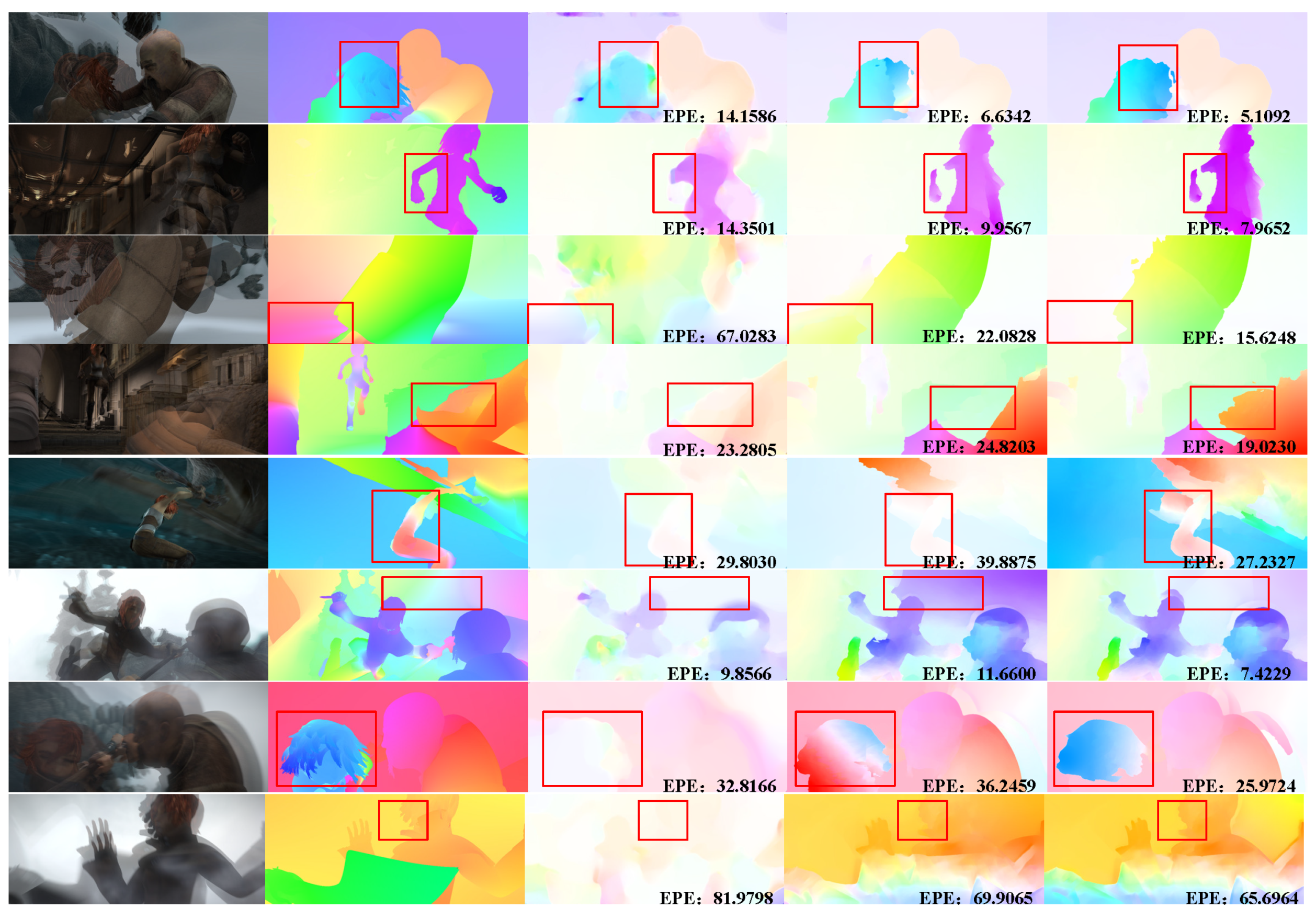
5.2. Experiments on Optical Flow

In our final experiment we compare the performance of our novel optical flow approach to other methods from literature. After detailed comparison with the current optical flow estimation methods in Table 2, the results of our method that is applied to several training sequences are given in Figure 8.
In Figure 8, we visualized the results of the LDOF algorithm, the FlowFields algorithm and our algorithm. LDOF is a classical optical flow field estimation algorithm. Because of its better robustness and less computational cost, it is widely used in practice. FlowFields is more sophisticated in design and performs well in the entire datasets, but it may have ‘strange errors’ in some cases due to its excessive dependence on neighborhood propagation. We use the red box to identify the contrast areas in Figure 8. We found that we can obtain better moving edges on either the clean data set (the first four rows) or the final data set (the last four rows). LDOF has a smooth phenomenon as a whole. Since the lack of occlusion detection, the FlowFields cannot reason accurate motion consistency areas. It is for this reason that the FlowFields algorithm in Figure 8 results in erroneous smoothing. For example, the foreground and background in the sixth row are not clearly distinguished, and the head in the seventh row is incorrectly divided into two areas.
Compared with the mainstream optical flow estimation algorithms, such as LODF and FlowFields, our method can obtain more accurate results on the entire dataset. Our method also surpasses most of the methods based on deep learning. Compared with MR-Flow [33], which ranks first in data set, our method can achieve comparable results while greatly reducing the computational cost. Specifically, it refers to the huge training data and hardware requirements generated in the training process of convolutional neural networks.

6. Conclusions

We presented an effective optical flow estimation algorithm based on reliable occlusion detection. First, we use various information for occlusion reasoning, and then propose a robust fusion strategy to obtain reliable occlusion results. Considering the difference between areas, we estimate the optical flow in the occlusion areas and the non-occlusion areas separately. Experiments on the MPI-Sintel dataset demonstrate that our approach effectively improves the accuracy of optical flow on overall images, and our approach are also competitive compared with those deep-learning-based algorithms. Furthermore, our proposed method can be combined with various methods. In this paper, the effect of occlusion detection on optical flow estimation is proved, and our method also provides reliable occlusion detection results. Therefore, in our future work, we will try to introduce our method into deep-learning, and it is hoped to improve the training efficiency and optical flow estimation accuracy of the network by providing reliable occlusion priori to remove interference during model training.

Author Contributions

Conceptualization, S.W. and Z.W.; Methodology, S.W. and Z.W.; Software, S.W.; Writing–original draft preparation, S.W.; Writing–review and editing, Z.W.; Supervision, Z.W.; Funding acquisition, Z.W.

Funding

This research was funded by National Natural Science Foundation of China (Grant Number: 61472393).

Conflicts of Interest

The authors declare no conflict of interest.

References

  1. Tsai, Y.H.; Yang, M.H.; Black, M.J. Video segmentation via object flow. In Proceedings of the IEEE Conference on Computer Vision and Pattern Recognition, Las Vegas, NV, USA, 27–30 June 2016; pp. 3899–3908. [Google Scholar]
  2. Baghaie, A.; Tafti, A.P.; Owen, H.A.; D’Souza, R.M.; Yu, Z. Three-dimensional reconstruction of highly complex microscopic samples using scanning electron microscopy and optical flow estimation. PLoS ONE 2017, 12, e0175078. [Google Scholar] [CrossRef] [PubMed]
  3. Mukherjee, K.; Mukherjee, A. Joint optical flow motion compensation and video compression using hybrid vector quantization. In Proceedings of the DCC’99 Data Compression Conference, Snowbird, UT, USA, 29–31 March 1999; p. 541. [Google Scholar]
  4. Lucas, B.D.; Kanade, T. An iterative image registration technique with an application to stereo vision. In Proceedings of the DARPA Image Understanding Workshop, 24–28 April 1981. [Google Scholar]
  5. Weinzaepfel, P.; Revaud, J.; Harchaoui, Z.; Schmid, C. DeepFlow: Large displacement optical flow with deep matching. In Proceedings of the IEEE International Conference on Computer Vision, Sydney, NSW, Australia, 1–8 December 2013; pp. 1385–1392. [Google Scholar]
  6. Bailer, C.; Taetz, B.; Stricker, D. Flow fields: Dense correspondence fields for highly accurate large displacement optical flow estimation. In Proceedings of the IEEE International Conference on Computer Vision, Las Condes, Chile, 7–13 December 2015; pp. 4015–4023. [Google Scholar]
  7. Brox, T.; Malik, J. Large displacement optical flow: descriptor matching in variational motion estimation. IEEE Trans. Pattern Anal. Mach. Intel. 2011, 33, 500–513. [Google Scholar] [CrossRef]
  8. Dosovitskiy, A.; Fischer, P.; Ilg, E.; Hausser, P.; Hazirbas, C.; Golkov, V.; Van Der Smagt, P.; Cremers, D.; Brox, T. Flownet: Learning optical flow with convolutional networks. In Proceedings of the IEEE International Conference on Computer Vision, Santiago, Chile, 7–13 December 2015; pp. 2758–2766. [Google Scholar]
  9. Ilg, E.; Mayer, N.; Saikia, T.; Keuper, M.; Dosovitskiy, A.; Brox, T. Flownet 2.0: Evolution of optical flow estimation with deep networks. In Proceedings of the IEEE Conference on Computer Vision and Pattern Recognition (CVPR), Honolulu, HI, USA, 21–26 July 2017. [Google Scholar]
  10. Ranjan, A.; Black, M.J. Optical flow estimation using a spatial pyramid network. In Proceedings of the IEEE Conference on Computer Vision and Pattern Recognition (CVPR), Honolulu, HI, USA, 21–26 July 2017. [Google Scholar]
  11. Thewlis, J.; Zheng, S.; Torr, P.H.; Vedaldi, A. Fully-trainable deep matching. arXiv 2016, arXiv:1609.03532. [Google Scholar]
  12. Žbontar, J.; Lecun, Y. Computing the tereo Mtching cost with a convolutional neural network. In Proceedings of the Computer Vision and Pattern Recognition, Boston, MA, USA, 7–12 June 2015; pp. 1592–1599. [Google Scholar]
  13. Gadot, D.; Wolf, L. Patchbatch: A batch augmented loss for optical flow. In Proceedings of the IEEE Conference on Computer Vision and Pattern Recognition, Las Vegas, NV, USA, 27–30 June 2016; pp. 4236–4245. [Google Scholar]
  14. Sevilla-Lara, L.; Sun, D.; Jampani, V.; Black, M.J. Optical flow with semantic segmentation and localized layers. In Proceedings of the IEEE Conference on Computer Vision and Pattern Recognition, Las Vegas, NV, USA, 27–30 June 2016; pp. 3889–3898. [Google Scholar]
  15. Bai, M.; Luo, W.; Kundu, K.; Urtasun, R. Exploiting semantic information and deep matching for optical flow. In Proceedings of the European Conference on Computer Vision, Amsterdam, The Netherlands, 11–14 October 2016; Springer: Cham, Switzerland, 2016; pp. 154–170. [Google Scholar]
  16. Shen, X.; Gao, H.; Tao, X.; Zhou, C.; Jia, J. High-quality correspondence and segmentation estimation for dual-lens smart-phone portraits. arXiv 2017, arXiv:1704.02205. [Google Scholar]
  17. Black, M.J.; Anandan, P. The robust estimation of multiple motions: Parametric and piecewise-smooth flow fields. Comput. Vis. Image Underst. 1996, 63, 75–104. [Google Scholar] [CrossRef]
  18. Bruhn, A.; Weickert, J.; Schnörr, C. Lucas/Kanade meets Horn/Schunck: Combining local and global optic flow methods. Int. J. Comput. Vis. 2005, 61, 211–231. [Google Scholar] [CrossRef]
  19. Lefebure, M.; Alvarez, L.; Esclarin, J.; Sánchez, J. A PDE model for computing the optical flow. In Proceedings of the XVI Congreso de Ecuaciones Diferenciales y Aplicaciones, Las Palmas de Gran Canaria, Spain, 21–24 September 1999; pp. 1349–1356. [Google Scholar]
  20. Alvarez, L.; Deriche, R.; Sanchez, J.; Weickert, J. Dense disparity map estimation respecting image discontinuities: A PDE and scale-space based approach. J. Vis. Commun. Image Represent. 2002, 13, 3–21. [Google Scholar] [CrossRef]
  21. Hur, J.; Roth, S. MirrorFlow: Exploiting symmetries in joint optical flow and occlusion estimation. In Proceedings of the International Conference on Computer Vision (ICCV), Venice, Italy, 22–29 October 2017. [Google Scholar]
  22. Kim, H.; Sohn, K. 3D reconstruction from stereo images for interactions between real and virtual objects. Signal Process. Image Commun. 2005, 20, 61–75. [Google Scholar] [CrossRef]
  23. Horn, B.K.; Schunck, B.G. Determining optical flow. Artif. Intel. 1981, 17, 185–203. [Google Scholar] [CrossRef]
  24. Anandan, P. A computational framework and an algorithm for the measurement of visual motion. Int. J. Comput. Vis. 1989, 2, 283–310. [Google Scholar] [CrossRef]
  25. Yang, Y.; Soatto, S. S2F: Slow-to-fast interpolator flow. In Proceedings of the Conference on Computer Vision and Pattern Recognition (CVPR), Honolulu, HI, USA, 21–26 July 2017. [Google Scholar]
  26. Weickert, J.; Bruhn, A.; Brox, T.; Papenberg, N. A survey on variational optic flow methods for small displacements. In Mathematical Models for Registration and Applications to Medical Imaging; Springer: Berlin/Heidelberg, Germany, 2006; pp. 103–136. [Google Scholar]
  27. Monzón, N.; Salgado, A.; Sánchez, J. Regularization strategies for discontinuity-preserving optical flow methods. IEEE Trans. Image Process. 2016, 25, 1580–1591. [Google Scholar] [CrossRef] [PubMed]
  28. Sun, D.; Roth, S.; Black, M.J. A quantitative analysis of current practices in optical flow estimation and the principles behind them. Int. J. Comput. Vis. 2014, 106, 115–137. [Google Scholar] [CrossRef]
  29. Brox, T.; Bruhn, A.; Papenberg, N.; Weickert, J. High accuracy optical flow estimation based on a theory for warping. In Proceedings of the European Conference on Computer Vision, Prague, Czech Republic, 11–14 May 2004; Springer: Berlin/Heidelberg, Germany, 2004; pp. 25–36. [Google Scholar]
  30. Alvarez, L.; Deriche, R.; Papadopoulo, T.; Sánchez, J. Symmetrical dense optical flow estimation with occlusions detection. Int. J. Comput. Vis. 2007, 75, 371–385. [Google Scholar] [CrossRef]
  31. Kennedy, R.; Taylor, C.J. Optical flow with geometric occlusion estimation and fusion of multiple frames. In Proceedings of the International Workshop on Energy Minimization Methods in Computer Vision and Pattern Recognition, Hong Kong, China, 13–16 January 2015; Springer: Cham, Switzerland, 2015; pp. 364–377. [Google Scholar]
  32. Chen, Q.; Koltun, V. Full flow: Optical flow estimation by global optimization over regular grids. In Proceedings of the IEEE Conference on Computer Vision and Pattern Recognition, Las Vegas, NV, USA, 27–30 June 2016; pp. 4706–4714. [Google Scholar]
  33. Wulff, J.; Sevilla-Lara, L.; Black, M.J. Optical flow in mostly rigid scenes. In Proceedings of the IEEE Conference on Computer Vision and Pattern Recognition (CVPR), Honolulu, HI, USA, 21–26 July 2017; Volume 2, p. 7. [Google Scholar]
  34. He, K.; Sun, J. Computing nearest-neighbor fields via propagation-assisted kd-trees. In Proceedings of the IEEE Conference on Computer Vision and Pattern Recognition, Providence, RI, USA, 16–21 June 2012; pp. 111–118. [Google Scholar]
  35. Luo, W.; Schwing, A.G.; Urtasun, R. Efficient deep learning for stereo matching. In Proceedings of the IEEE Conference on Computer Vision and Pattern Recognition, Las Vegas, NV, USA, 27–30 June 2016; pp. 5695–5703. [Google Scholar]
  36. Revaud, J.; Weinzaepfel, P.; Harchaoui, Z.; Schmid, C. Epicflow: Edge-preserving interpolation of correspondences for optical flow. In Proceedings of the IEEE Conference on Computer Vision and Pattern Recognition, Boston, MA, USA, 7–12 June 2015; pp. 1164–1172. [Google Scholar]
  37. Dollár, P.; Zitnick, C.L. Structured forests for fast edge detection. In Proceedings of the IEEE International Conference on Computer Vision, Sydney, Australia, 1–8 December 2013; pp. 1841–1848. [Google Scholar]
  38. Achanta, R.; Shaji, A.; Smith, K.; Lucchi, A.; Fua, P.; Süsstrunk, S. SLIC superpixels compared to state-of-the-art superpixel methods. IEEE Trans. Pattern Anal. Mach. Intel. 2012, 34, 2274–2282. [Google Scholar] [CrossRef] [PubMed]
  39. Blake, A.; Zisserman, A. Visual Reconstruction; MIT Press: London, UK, 1987. [Google Scholar]
  40. Wainwright, M.J.; Jaakkola, T.S.; Willsky, A.S. MAP estimation via agreement on trees: message-passing and linear programming. IEEE Trans. Inf. Theory 2005, 51, 3697–3717. [Google Scholar] [CrossRef]
  41. Kolmogorov, V. Convergent tree-reweighted message passing for energy minimization. IEEE Trans. Pattern Anal. Mach. Intel. 2006, 28, 1568–1583. [Google Scholar] [CrossRef] [PubMed]
  42. Pérez, J.S.; López, N.M.; de la Nuez, A.S. Robust optical flow estimation. Image Process. Line 2013, 3, 252–270. [Google Scholar] [CrossRef]
  43. Butler, D.J.; Wulff, J.; Stanley, G.B.; Black, M.J. A naturalistic open source movie for optical flow evaluation. In Proceedings of the European Conference on Computer Vision, Florence, Italy, 7–13 October 2012; Springer: Berlin/Heidelberg, Germany, 2012; pp. 611–625. [Google Scholar]
  44. Wang, Y.; Yang, Y.; Yang, Z.; Zhao, L.; Wang, P.; Xu, W. Occlusion aware unsupervised learning of optical flow. In Proceedings of the IEEE Conference on Computer Vision and Pattern Recognition, Salt Lake City, UT, USA, 18–23 June 2018; pp. 4884–4893. [Google Scholar]
Figure 1. Algorithm overview. Given adjacent frames, we first compute matching results and edge detection results. Then three kinds of information are used to obtain occlusion detection respectively. Next, our fusion strategy is adopted to obtain robust occlusion detection results. Finally, the whole image is divided into occlusion and non-occlusion and estimated optical flow separately.
Algorithms 12 00092 g001
Figure 2. Flow diagram of our matching-based strategy.
Algorithms 12 00092 g002
Figure 3. Flow diagram of our warped image-based strategy.
Algorithms 12 00092 g003
Figure 4. The flowchart of our warped image-based strategy.
Algorithms 12 00092 g004
Figure 5. Flow diagram of our edge-based strategy.
Algorithms 12 00092 g005
Figure 6. Flow diagram of our multi-source information fusion strategy.
Algorithms 12 00092 g006
Figure 7. Occlusion detection on the MPI-Sintel dataset (final version). From top to bottom: overlaid input frames, ground truth, the results of matching-based strategy, the results of warped image-based strategy, the results of edge-based strategy, the results of initial fusion, the results of partial fusion and the results of final fusion. The F-measure is printed in the image.
Algorithms 12 00092 g007
Figure 8. Optical flow estimation on the MPI-Sintel dataset. The first four rows are the result of clean version, and the last four rows are the result of final version. From left to right: overlaid input frames, ground truth, the results of LDOF, the results of FlowFields and the results of our method. For all methods, we use the red box to identify the contrast areas and the endpoint error(EPE) is printed in the image.
Algorithms 12 00092 g008
Table 1. F-measure and AEE of different strategies.
MethodsF-MeasureAEE
M m 0.29193.8244
M w 0.45343.7604
M e 0.11674.1567
M i n i t 0.44833.7828
M w + 0.44723.7760
M0.47153.7440
M w a n g [44]0.486.34
Table 2. Quantitative evaluation of our method.
MethodsAEE_CleanAEE_Final
FlownetS [8]4.505.45
FlownetC [8]4.315.87
SPyNet [10]4.125.57
MR-Flow [33]1.833.59
classic+NLP [28]4.135.90
DeepFlow [5]2.663.57
EpicFlow [36]2.273.56
FlowFileds [6]2.133.82
LDOF [7]4.326.21
ours2.093.74

