Article

Bamboo Garden Trimming Problem: Priority Schedulings †

by
Mattia D’Emidio
1,*,
Gabriele Di Stefano
1 and
Alfredo Navarra
2
1
Department of Information Engineering, Computer Science and Mathematics, University of L’Aquila; 67100 L’Aquila, Italy
2
Department of Mathematics and Computer Science, University of Perugia, 06123 Perugia, Italy
*
Author to whom correspondence should be addressed.
This paper is an extended version of our paper published in the 45th International Conference on Current Trends in Theory and Practice of Computer Science (SOFSEM), Nový Smokovec, Slovakia, 27–30 January 2019.
Algorithms 2019, 12(4), 74; https://doi.org/10.3390/a12040074
Submission received: 18 January 2019 / Revised: 4 April 2019 / Accepted: 11 April 2019 / Published: 13 April 2019

Abstract

:
The paper deals with the Bamboo Garden Trimming (BGT) problem introduced in [Gąsieniec et al., SOFSEM’17]. The problem is difficult to solved due to its close relationship to Pinwheel scheduling. The garden with n bamboos is an analogue of a system of n machines that have to be attended (e.g., serviced) with different frequencies. During each day, bamboo b i grows an extra height h i , for i = 1 , , n and, on the conclusion of the day, at most one bamboo has its entire height cut.The goal is to design a perpetual schedule of cuts to keep the height of the tallest ever bamboo as low as possible. The contribution in this paper is twofold, and is both theoretical and experimental. In particular, the focus is on understanding what has been called priority schedulings, i.e., cutting strategies where priority is given to bamboos whose current height is above a threshold greater than or equal to H = i = 1 n h i . Value H represents the total daily growth of the system and it is known that one cannot keep bamboos in the garden below this threshold indefinitely. As the first result, it is proved that, for any distribution of integer growth rates h 1 , , h n and any priority scheduling, the system stabilises in a fixed cycle of cuts. Then, the focus is on the so-called ReduceMax strategy, a greedy priority scheduling that each day cuts the tallest bamboo, regardless of the growth rates distribution. ReduceMax is known to provide a O ( log n ) -approximation, with respect to the lower bound H. One of the main results achieved is that, if ReduceMax stabilises in a round-robin type cycle, then it guarantees 2-approximation. Furthermore, preliminary results are provided relating the structure of the input instance, in terms of growth rates, and the behavior of ReduceMax when applied to such inputs. Finally, a conjecture that ReduceMax is 2-approximating for the BGT problem is claimed, hence an extended experimental evaluation was conducted to support the conjecture and to compare ReduceMax with other relevant scheduling algorithms. The obtained results show that ReduceMax : (i) provides 2-approximation in all considered inputs; and (ii) always outperforms other considered strategies, even those for which better worst case approximation guarantees have been proven.

1. Introduction

This paper deals with a perpetual scheduling problem in which n machines, denoted later as bamboos, need to be attended with possibly known and likely different frequencies. In other words, some machines may have to be attended more often than others. This problem was proposed and studied by [1] under the name of Bamboo Garden Trimming (BGT) problem. Given is a collection (garden) of n bamboos b 1 , b 2 , …, b n along with respective daily growth rates h 1 , h 2 , …, h n greater than 0. The authors of [1] assumed that, initially, the height of each bamboo is set to zero, whereas in this paper bamboos are allowed to start with arbitrary heights.
The robotic gardener maintaining the garden trims one bamboo per day to height zero according to some predefined schedule. The main goal in BGT is to design perpetual schedules of cuts which keep the height of the tallest ever bamboo as low as possible. The main constraints are that the gardener is allowed to cut exactly one (of their choice) bamboo at the end of each day and is not allowed to attend the garden at any other times. Once the gardener has decided which bamboo to trim at the end of the current day (which corresponds to one round in the schedule), the action of actual trimming is instantaneous. Different variants of the problem have been defined [1], but, in its “easiest” representation, all data are available to the gardener, i.e., one knows how many bamboos form the garden and for each bamboo what is the daily growth rate. Hence, one may think about trimming strategies that consider all the data, or simply choosing the bamboo to be trimmed according with the current status of the garden.
The problem reveals a combinatorial beauty, also related to the easiness of its definition that rapidly allows to start thinking about trimming strategies. As a first thought, it usually appears surprising that that the problem comes out to be of difficult resolution. This further motivates the design of different and efficient trimming strategies, varying on the usage of the available data. Moreover, the interest to this problem comes from its close relation with fundamental scheduling problems, e.g., Pinwheel scheduling.
The Pinwheel problem [2] is defined as follows. Given a set V = f 1 , f 2 , , f n of positive integers called Pinwheel frequencies, one is asked to create an infinite sequence S of indices drawn from the set 1, 2, , n, such that, any sub-sequence of f i V consecutive elements in S includes at least one index i. The density of set V is defined as D = i = 1 n 1 f i and it is known that instances having density D > 1 cannot be scheduled. An example of input instance for the Pinwheel problem is shown in Figure 1.
In [2], it has been shown that Pinwheel is NP-hard assuming succinct representation of the problem, whereas it can be efficiently solved when the Pinwheel frequencies are powers of 2 and the density is at most 1 [1,3]. In [1], a 2-approximation algorithm for BGT, based on the resolution of the Pinwheel problem in the special case where frequencies are powers of 2 and the density is at most 1, has been introduced. In more details, given an instance of BGT with rates { h 1 , h 2 , , h n } , one can create a parametrical instance I ( δ ) of Pinwheel with frequencies
f i = ( 1 + δ ) H h i , for i = 1 , 2 , , n and for any δ > 0
and prove that a (feasible) solution to I ( δ ) implies a ( 1 + δ ) -approximation schedule for the original BGT instance. In particular, one can set δ = 1 and round frequencies to closest power of two to obtain an instance of Pinwheel having power of two frequencies and density D 1 , that can be scheduled efficiently by a greedy algorithm. We refer the interested reader to [1,3] for more details on the proofs.
Furthermore, a 4-approximation and an O ( log n ) -approximation algorithms have been provided, in the case the gardener exploits only partial knowledge of the input instance. In detail, to achieve the 4-approximation, it is sufficient to know for any couple of bamboos which one is associated with the highest growth rate, without knowing the exact rates. To achieve the O ( log n ) -approximation, instead, no knowledge about growth rates is assumed. Here, the interest is more related to this last setting, with the aim to improve the approximation ratio to a constant.

1.1. Related Work

The BGT problem, while of independent combinatorial interest, originates from perpetual testing of virtual machines in cloud systems [4]. In such systems, the frequency in which virtual machines are tested for undesirable symptoms varies depending on the importance of dedicated cloud operational mechanisms. The BGT problem considered here is also a close relative of several classical algorithmic problems which focus on monitoring including Graph Exploration [5,6,7,8], Art Gallery Problem [9] and its dynamic extension k-Watchmen Problem [10]. In the work on Patrolling [11,12], the studies focus on monitoring a set of points with the same frequency of attendance, whereas in [13], the frequency may vary.
In this paper, similarly to [1], the focus is on the case where each bamboo has its own attendance factor, which makes it related to periodic scheduling [14], several variants of Pinwheel related problems [2,15,16,17] including periodic Pinwheel problem [18,19] and Pinwheel scheduling [20], as well as the concept of P-fairness in sharing multiple copies of some resource among various tasks [21,22]. It is worth pointing out here that the intractability of BGT results from the hardness of Pinwheel scheduling proved in [23].
Of course, the relevance of a new variant of scheduling is of main interest to the algorithmic community as scheduling issues represent fundamental primitives in many contexts. To this respect, it is worth citinh the close relation of the proposed BGT problem with the work done on similar settings in [24,25]. The main difference basically resides in the objective function. In fact, in [24,25], the aim is to minimise the long-run average height of the bamboos, whereas in BGT the aim concerns the minimisation of the maximum height ever reached by the bamboos.
In related research on minimising the maximum occupancy of a buffer in a system of n buffers, the usual setting is a game between the player and the adversary [26,27,28]. The adversary decides how a fixed total increase of data in each round is distributed among the buffers and tries to maximise the maximum occupancy of a buffer. The player decides which buffer (or buffers) should be emptied next and tries to minimise the maximum buffer size. The upper bounds developed in this more general context can be translated into upper bounds for the BGT problem. However, here the aim is to derive tighter bounds for the case where the knowledge of growth rates is not exploited, hence adopting strategies able to deal with input data being either partially or entirely unknown.
Probably the most natural algorithm to keep the elevation of the bamboo garden low is the greedy approach of always cutting the currently tallest bamboo. This method, which is agnostic with respect to growth rates, was first coined in [4] under the name of ReduceMax and further studied in [1]. This strategy was also considered independently (and under a different name) in the adversarial setting of buffer minimisation problems [27]. Another method studied in [1] is the ReduceFastest 2 approach, in which the fastest growing bamboo is cut but only among those having height above the threshold 2 H , where
H = i = 1 n h i .
Value H represents the total daily growth of the system of bamboos and it is known [1] that one cannot keep bamboos below this threshold level. From [1], it is known that ReduceFastest 2 provides a constant approximation to BGT, i.e., none of the bamboos grows above height 4 H . However, its applicability depends on the knowledge of value H and at least an ordering of the bamboos with respect to their growth rates. More interestingly, ReduceMax does not require such a knowledge but surprisingly it is not well understood. While there are insights that it should perform better than ReduceFastest 2 , the only upper bound known for the maximum height of bamboos is O ( H · log n ) [1].

1.2. Achieved Results

In this paper, the main contribution is twofold, and it refers to both theoretical and experimental studies on the BGT problem. In particular, the focus is on better understanding of what are called priority schedulings that operate on any “reasonable”, i.e., involving all bamboos, strategy of cuts in which priority is given to bamboos with the current height above a threshold greater than or equal to H. Both ReduceMax and ReduceFastest 2 fall into the priority category. Moreover, one further requirement is that scheduling strategies must be fully deterministic. Hence, in the case of ties, i.e., when two or more bamboos are eligible to be cut with respect to the considered strategy, the bamboo with the biggest index is selected.
As the first result, it is proved that, for any distribution of integer growth rates h 1 , , h n , and any priority scheduling, the system stabilises in a fixed cycle of cuts, eventually. However, the time needed to converge depends on the initial heights of bamboos. Then, it is shown that, whenever ReduceMax stabilises in a round-robin type cycle, it guarantees 2-approximation for BGT. Finally, extended experiments are conducted to compare ReduceMax with other strategies, including ReduceFastest 2 . Note that the work in [4] contains some experiments on ReduceMax , focusing only on selected distributions of bamboo growth rates. In contrast, here the focus is on all possible distributions of bounded size. The experiments show ReduceMax being 2-approximating in all considered instances, and provide evidence that ReduceMax outperforms all other tested strategies. Consequently, we conjecture the following.
Conjecture 1.
Algorithm ReduceMax is 2-approximating for the BGT problem.
Note that, the results presented in this paper have appeared in a preliminary form in [29].

2. Notation

Given is a collection { b 1 , b 2 , , b n } of n bamboos (i.e., a garden) along with respective daily growth rates h 1 , h 2 , …, h n . It is assumed that each h i is a positive integer, for any 1 i n , and call a configuration C t the sequence ( 1 t , 2 t , , n t ) of the bamboos’ heights at a given day t. Any configuration C t = ( 1 t , 2 t , , n t ) is determined by a growth mechanism applied on its predecessor C t 1 = ( 1 t 1 , 2 t 1 , , n t 1 ) , i.e., for any 1 i n , it holds i t = i t 1 + h i . The only exception to this behavior is what is called a trimming operation. In particular, a bamboo b i is said to be trimmed (equivalently cut) at a given day t if the height i t is reduced to zero and hence, trivially, i t + 1 = h i . For the sake of simplicity, in what follows the term t is omitted from all notations when the number of the day is clear from the context. Finally, given a configuration C, let V ( C ) denote the volume of configuration C, which is the sum of all bamboos’ heights in C, i.e.,
V ( C ) = i = 1 n i .
An input instance I to the BGT problem is a set of growth rates { h i } 1 i n , complemented by the initial configuration C 0 . The interest is in the design of perpetual schedules of cuts, which allow keeping the tallest bamboo in the garden as low as possible. In particular, it is assumed that at most one trimming operation can take place every day. Therefore, the aim at designing an algorithm A that, for a given input instance I, computes a perpetual schedule A ( I ) = ( i 1 , i 2 , ) , i.e., a sequence of indices i j { 0 , 1 , 2 , , n } that determines, for any day t > 0 , the bamboo to be trimmed, unless i j = 0 when no bamboo is cut. In other words, a schedule of this kind defines an ordered sequence of trimming operations on the bamboos. In what follows, an algorithm determining perpetual schedules is called a perpetual scheduling, or simply scheduling algorithm.
Given an input instance I and a perpetual scheduling S , an execution E ( I , S ) is the sequence ( C 0 , C 1 , ) obtained by applying the schedule computed by S on C 0 . Moreover, given an execution E and a configuration C, let M ( E ) ( M ( C ) , respectively) denote the maximum height reached by a bamboo in E (C, respectively). Finally, let H = i = 1 n h i denote the sum of the growth rates. It is known that no algorithm can compute a schedule that keeps the heights of all the bamboos below H indefinitely (i.e., such that M ( E ) < H ) [1].

3. Theoretical Results

In this section, first a formal definition of priority schedulings along with the analysis of their performance (see Section 3.1) are introduced. Then, the focus is on the strategy ReduceMax and on showing that it provides 2-approximation for BGT under specific assumptions (see Section 3.2).

3.1. Priority Schedulings

Let C be the set of any configuration of n bamboos.
Definition 1.
An oblivious scheduling σ : C { 0 , 1 , , n } is a function which for any configuration of heights in C returns an index i of the bamboo to be cut, and i = 0 means that none of the bamboos is scheduled to be cut.
In other words, in oblivious schedulings the next cut is solely based on the current configuration, without exploiting any knowledge about past cuts.
Definition 2.
A configuration C = ( 1 , 2 , , n ) is said to be ordered whenever i < j implies h i h j .
The above implies the order of the sequence in C reflects a non-increasing ordering of the growth rates, i.e., 1 is the height of the bamboo with the biggest growth rate.
Definition 3.
An ordered oblivious scheduling σ : O { 0 , 1 , , n } is an oblivious scheduling where O C is the set of ordered configurations in C .
Definition 4.
Given a threshold τ H and any (ordered) configuration C C , let L be the set of indices of all bamboos whose height is strictly greater than τ. An oblivious scheduling σ τ is a (ordered) τ- priority scheduling if and only if L implies σ τ ( C ) L .
In the remainder of the paper, a (ordered) τ -priority scheduling is simply referred to as a priority scheduling when the ordering and the value of τ are either clear from the context or irrelevant. Clearly, ReduceFastest 2 is an ordered 2 H -priority scheduling, as it cuts only bamboos above threshold 2 H on the basis of the ordering of the growth rates. For ReduceMax , instead, it can be proved it is a priority scheduling regardless of the ordering of the bamboos’ growth rates. This means it can be applied to a wider range of input configurations, not only to ordered ones, as required by ReduceFastest 2 .
Fact 1.
ReduceMax is a priority scheduling.
Proof. 
Given any threshold τ H (as required by Definition 4) each day ReduceMax cuts the tallest bamboo. This includes also the case when there are bamboos taller than τ . This in turn means that ReduceMax gives priority to bamboos higher than τ , if any. □
The next lemma gives an upper bound on the volume the garden may reach in a priority scheduling. This is useful to prove that any priority scheduling stabilises into a cycle of finite length.
Lemma 1
(Upper Bound on Volume). Given a τ-priority scheduling σ τ and an input I, there exists a time t , such that, for any t > t , it holds V ( C t ) n τ , where C t E ( I , σ τ ) .
Proof. 
First, assume that M ( E ( I , σ τ ) ) > τ , as otherwise V ( C ) n τ , for each C E ( I , σ τ ) , and the lemma holds. If it is also assumed M ( C 0 ) > τ then it is possible to prove that, within finite time, a configuration C with M ( C ) τ is reached by applying σ τ . In particular, note that for as long as there are bamboos having height greater than τ , the total volume decreases each day, being τ H , of at least 1. Thus, there must exist a time t when eventually M ( C t ) τ , since the volume cannot decrease indefinitely. At this time, it holds V ( C t ) n τ .
Therefore, let t > t be the first day after time t such that C t has a bamboo having height greater than τ . Clearly, V ( C t ) < V ( C t 1 ) τ + H , as σ τ cuts a bamboo with height greater than τ and, at the end of the day, all bamboos grow by H in total. Moreover, by hypothesis V ( C t 1 ) n τ , since i τ , for each i C t 1 . Hence,
V ( C t ) < ( n 1 ) τ + H n τ
as H τ . Now, by focussing on V ( C t + 1 ) , since in C t the scheduling algorithm cuts a bamboo having height bigger than τ , and since the sum of daily growths is exactly H, it follows that V ( C t + 1 ) < V ( C t ) . This is actually true for any following configuration until day t where i τ for any i C t . Notice that in t , the same set of hypotheses as of day t hold, then by repeating the reasoning, the claim follows. □
By Lemma 1, the next corollary can be obtained, which guarantees that any priority scheduling stabilises into a cycle of finite length, i.e., that the sequence of cuts becomes periodic.
Corollary 1
(Existence of a Cycle). Given a τ-priority scheduling σ τ and an input I, there exist two days t and t , where t < t , C t = C t , and C t , C t E ( I , σ τ ) .
Proof. 
The claim follows from Lemma 1, since the number of configurations having volume at most n τ is finite. □
By the above corollary, it follows that any priority scheduling stabilises in a cycle, eventually. In fact, by Definition 1, a priority scheduling (which is an oblivious scheduling) computes the same trimming operation if the same configuration shows up again. It is worth reminding that, in the case of ties, the bamboo having the biggest index is cut. In this paper, the focus is on the properties of such cycles, as they represent the perpetual trimming process that have to be executed indefinitely. Hence, the trend will be to disregard configurations preceding L E where, given an execution E, L E denotes its periodic part (i.e., the sequence of configurations in the cycle). In particular, to better characterise such cycles, the next notation is introduced:
  • L E = ( C 1 = C t , C 2 = C t + 1 , C 3 , , C λ E ) , where C t is the first configuration belonging to L E , reached from C 0 , and λ E = | L E | is the length of the cycle, i.e., the number of configurations in L E .
  • l t is the height of the bamboo cut in C t L E . It is assumed l t = 0 if no bamboo is cut.
  • c i is the number of times bamboo b i is cut in L E , for each i = 1 , , n , which is equal to the number of relative maximum heights reached by b i in the cycle.
  • m i j is the relative maximum height reached by b i in the cycle just before the jth cut, for i = 1 , , n and j = 1 , , c i . Note that, by definition, during day t, l t = m i j for some values of i and j.
  • M i = j = 1 c j m i j is the sum of the relative maximum heights reached by b i .
The next lemma provides a very useful property of the cuts that are performed within a cycle of a priority scheduling. In particular, it can be shown that the average value of heights reached by bamboos in L E , just before a cut, is always H. As shown below, the lemma is exploited to prove that within some specific circumstances ReduceMax is a 2-approximation algorithm.
Lemma 2
(On Average Height of Cuts within a Cycle). Given an execution E of a priority scheduling, then 1 λ E t = 1 λ E l t = H .
Proof. 
Let Δ V t = V ( C t ) V ( C t 1 ) be the change of the volume from C t 1 to C t , for any t = 1 , λ E . C 0 C λ E , since cycle L E exists by Corollary 1. Thus, it holds Δ V t = H l t , because at day t the bamboo of height l t is cut and all bamboos grow by H in total. Now, since t = 1 λ E Δ V t must be equal to zero, as configurations in L E come periodically, then:
t = 1 λ E Δ V t = t = 1 λ E ( H l t ) = λ E · H t = 1 λ E l t = 0 .
Therefore, it is obtained that
t = 1 λ E l t = λ E · H
and the claim holds. □
The next lemma as well as the subsequent corollary are not exploited in the rest of the paper as the focus is on analysing the performance of ReduceMax . However, such results constitute interesting and elegant properties characterising general priority schedulings, hence they are worth being reported. In particular, in what follows, the length of L E is characterised in terms of the maximum height reached by any bamboo having growth rate equal to h i .
Lemma 3
(Characterisation of λE). Given an execution E of a priority scheduling and an index i { 1 , 2 , , n } , then
λ E = M i h i .
Proof. 
Let p i j = m i j / h i . The value of p i j is an integer representing the number of days between the jth cut of b i and the previous one. Then,
M i = j = 1 c j m i j = j = 1 c j h i · p i j = h i · j = 1 c j p i j = h i · λ E .
An immediate consequence is the following corollary.
Corollary 2
(Properties of Rates and Maximum Heights). Given an execution E of a priority scheduling, and two indices i , j { 1 , 2 , , n } , then:
M i M j = h i h j .

3.2. ReduceMax Scheduling

In this section, the focus is on ReduceMax . The aim is to show that ReduceMax performs better than an O ( log n ) -approximation algorithm. Actually, the approximation ratio is improved only for a specific set of input instances, by also exploiting some results achieved for priority schedulings. The results contained in this section constitute a path toward a partial achievement of the aim, leading to a 2-approximation ratio for ReduceMax when confined to some specific instances. By Fact 1, it en shown above that ReduceMax is a priority scheduling, regardless of the chosen threshold τ H required by Definition 4. It follows that ReduceMax inherits all results obtained in the previous section for priority schedulings. In particular, given an execution E obtained by applying ReduceMax , let l t be the height of the bamboo cut in C t L E , i.e., l t = M ( C t ) , and let M E ¯ = 1 λ E t = 1 λ E l t denote the average of the maximum heights reached by bamboos in L E . Then, for ReduceMax , Lemma 2 can be reformulated as follows.
Corollary 3
(On Average Height of Cuts of ReduceMax). Let E be an execution of ReduceMax . Then, M E ¯ = H .
A natural intuitive property is provided in the next lemma.
Lemma 4
(On the Amounts of Cuts within a Cycle). Let E be an execution of ReduceMax . For any two indices i , j { 1 , 2 , , n } such that h i h j , it holds c i c j .
Proof. 
By contradiction, assume that c i < c j . Then, in cycle L E there must be at least two cuts of b j between two consecutive cuts of b i . However, since h i h j , b j after the first cut will grow less than b i and it will never reach b i before its second cut, which is a contradiction. □
A direct consequence of Lemma 4 is that, if two bamboos exhibit the same growth rate, they also have the same number of cuts in the cycle.
Corollary 4
(Sufficient Condition for Same Number of Cuts). If E is an execution of ReduceMax , h i = h j implies c i = c j .
Let m i = max { m i j : j = 1 , 2 , , c i } be the maximum height reached by bamboo b i in a cycle L E of ReduceMax . The next result shows that c i = 1 suffices to guarantee m i < 2 H . Basically, the next lemma guarantees that the approximation factor of ReduceMax reduces from O ( log n ) [1] to 2 if all bamboos are cut only once within the cycle, i.e., when the cycle of ReduceMax is equivalent to the round-robin strategy.
Lemma 5
(Sufficient Condition for Bounded Maximum). Let E be an execution of ReduceMax . Then,
c i = 1 for some i { 1 , 2 , , n } m i < 2 H .
Proof. 
First, notice that c i = 1 suffices to immediately obtain m i = λ E · h i . Moreover, by Corollary 3 it holds M E ¯ = H , i.e., that λ E · H t = 1 λ E l t = 0 .
Now, it is known that b i is cut only once and, as L E is periodic, C 1 is equal to the configuration where the height of bamboo b i is h i . Thus, each term l t is trivially lower bounded by the height of bamboo b i at day t, i.e., l t t · h i . Hence, λ E · H t = 1 λ E t · h i 0 . Therefore, it holds that
λ E · H t = 1 λ E t · h i λ E · ( λ E + 1 ) 2 · h i
which implies
λ E 2 2 · h i + λ E 2 · h i λ E · H 0
that is
λ E · h i + h i 2 · H 0 .
This in turn implies
λ E · h i < 2 H
and hence m i < 2 H . □
If c i = 1 , for some i = 1 , 2 , n , then similar to the proof of Lemma 5, a limit on the value of λ E can be obtained, as summarised by the following corollary.
Corollary 5
(Sufficient Condition for Bounded Length of Cycles). Let E be an execution of ReduceMax . Then,
c i = 1 for some i { 1 , 2 , , n } λ E 2 · H h i 1 .
Given the above results, and an execution E, configurations where the bamboo having the largest growth rate, e.g., b m , such that c m = 1 , are now characterised. By Lemma 4, c m = 1 directly implies c i = 1 for all i = 1 , 2 , n .
To this aim, given the set of growth rates h 1 , h 2 , …, h n , the next notation is used, by: (i) h ( k ) , k [ 1 , n ] , its kth order statistic, that is the kth smallest value in an ordered view of the set (e.g., h ( 1 ) denotes the smallest rate while h ( n ) denotes the largest one); and (ii) b ( k ) , k [ 1 , n ] , the bamboo associated with h ( k ) . Moreover, given an execution E, c ( k ) ( m ( k ) , respectively), k [ 1 , n ] , denote the number of times bamboo b ( k ) is cut (the maximum height reached by b ( k ) , respectively) in L E . The next result can be now proved.
Lemma 6
(Characterising Configurations Having c ( n ) = 1 ). Given an input I, let E be an execution of ReduceMax . Then:
c ( n ) = 1 h ( k ) h ( k + 1 ) 1 1 n where k { 1 , 2 , n 1 } .
Proof. 
( ) Since c ( n ) = 1 , by Lemma 4, it is known that c i = 1 for any i = 1 , 2 , n and then λ E = n . Hence, the maximum height reached by bamboo b ( n ) is m ( n ) = n · h ( n ) , at day n. This means that there exists a bamboo b i b ( n ) , such that, at day n 1 , bamboo b i has length larger than b ( n ) , i.e., m i = n · h i ( n 1 ) · h ( n ) . Consequently, given h ( n ) h ( n 1 ) h i , it follows that n · h ( n 1 ) ( n 1 ) · h ( n ) and hence:
h ( n 1 ) h ( n ) n 1 n
By the same reasoning as above, when bamboo b ( n 1 ) reaches its maximum length m ( n 1 ) = h ( n 1 ) · n , there must exist another bamboo b j , such that b j b ( n ) , b j b ( n 1 ) and m j = n · h j ( n 1 ) · h ( n 1 ) . Given that h ( n ) h ( n 1 ) h ( n 2 ) h j , it follows that n · h ( n 2 ) ( n 1 ) · h ( n 1 ) and hence:
h ( n 2 ) h ( n 1 ) n 1 n .
In general, the above reasoning can be iterated up to n times to obtain:
h ( k ) h ( k + 1 ) n 1 n = 1 1 n
and the first implication of the claim follows.
( ) By construction, it is possible to build L E = ( C 1 , C 2 , , C n ) of an execution E such that c i = 1 for each i = 1 , 2 , n . Now, let
C 1 = ( 1 · h ( n ) , 2 · h ( n 1 ) , , ( n 1 ) · h ( 2 ) , n · h ( 1 ) ) .
Since
h ( k ) h ( k + 1 ) 1 1 n
for any k { 1 , 2 , n 1 } , it follows that
( k + 1 ) · h ( k ) k · h ( k + 1 )
for each k { 1 , 2 , n 1 } . In fact, it holds
( k + 1 ) · h ( k ) ( k + 1 ) · 1 1 n · h ( k + 1 ) = ( k + 1 ) · h ( k + 1 ) k + 1 n · h ( k + 1 ) k · h ( k + 1 ) .
Then, in C 1 , bamboo b ( 1 ) is cut and the resulting configuration is
C 2 = ( 2 · h ( n ) , 3 · h ( n 1 ) , , n · h ( 2 ) , 1 · h ( 1 ) ) .
By a simple algebraic manipulation, it is possible to infer that in C 2 the maximal bamboo height is n · h ( 2 ) , and hence bamboo b ( 2 ) is cut.
In general, for t = 1 , 2 , , n , it holds
C t = ( t · h ( n ) , ( t + 1 ) · h ( n 1 ) , , n · h ( t ) , 1 · h ( t 1 ) , 2 · h ( t 2 ) , , ( t 1 ) · h ( 1 ) )
and, in C t , the resulting bamboo that is cut is b ( t ) , having height n · h ( t ) . In fact, in C t , the height of bamboo b ( t ) is straightforwardly larger than that of any bamboo b ( i ) for i < t . For i > t , instead, since the height of bamboo b ( i ) is ( t + i ) · h ( i ) , it follows, by a similar argument as above, that ( t + i ) · h ( i ) ( t + i 1 ) · h ( i + 1 ) , hence b ( t ) is the bamboo exhibiting the maximal height in C t .
When t = n , it is possible to observe that C t = ( n · h ( n ) , 1 · h ( n 1 ) , 2 · h ( n 2 ) , , ( n 1 ) · h ( 1 ) ), where clearly b ( n ) has the maximal height and it is cut, leading to a new configuration which coincides with C 1 . □
Reminding that, when dealing with ReduceMax , it is not required to have bamboos ordered according to their growth rates, in what follows, executions having c ( n ) = 1 are considered as minimum-cycle executions, since c ( n ) = 1 implies that c i = 1 for any bamboo b i , and then the execution exhibits a minimum-length cycle, that is λ E = n . Note that λ E cannot be smaller than n, as each bamboo must be cut at least once. These observations are summarised in the next corollary.
Corollary 6
(Characterisation of Minimum-cycle Executions). Let E be an execution of ReduceMax . Then,
c ( n ) = 1 λ E = n .
Finally, the next corollary can be also obtained for minimum-cycle executions of ReduceMax .
Corollary 7
(On the Maximum Height in Minimum-cycle Executions). Let E be an execution of ReduceMax . If E is a minimum-cycle execution, then M ( L E ) < 2 H .
Proof. 
In a minimum-cycle execution, the maximum height reached by a bamboo b i is exactly m i = n h i . Hence, the maximum height reached during an execution by any bamboo is due to h ( n ) and, in particular, is given by M ( L E ) = m ( n ) = n · h ( n ) . Hence, the thesis is an immediate consequence of Lemma 5, as c ( n ) = 1 . □
Corollary 7 is of particular interest, since by Conjecture 1 it has been essentially stated that M ( E ) < 2 H for all the executions E obtained via ReduceMax . Hence, Corollary 7 represents a partial proof to the conjecture, holding for the case of minimum-cycle executions. In the next section, the validity of the posed conjecture on a large set of inputs is experimentally evaluated.
Clearly, minimum-cycle executions are desirable as they guarantee M ( E ) < 2 H . However, from a practical view point, round-robin schedulers are not always the most desirable solutions as different properties and requirements might be involved. In particular, the following result provides a sufficient condition for non-minimum cycle executions.
Theorem 1
(Sufficient Condition for Non-minimum-cycle Executions). Given an input I, let E be an execution obtained via ReduceMax . Then, E is not a minimum-cycle execution if
h ( 1 ) h ( n ) > e
where e is Euler’s number.
Proof. 
By contradiction, assume that h ( 1 ) h ( n ) > e holds in E and that c ( n ) = 1 , i.e., E is a minimum-cycle execution. Then, by Lemma 6, it holds
h ( i ) h ( i + 1 ) 1 1 n , i { 1 , 2 , n 1 }
which implies
h ( i + 1 ) h ( i ) 1 1 1 n = 1 + 1 n 1
and hence
h ( n ) h ( 1 ) = h ( n ) h ( n 1 ) · h ( n 1 ) h ( n 2 ) · h ( n 2 ) h ( n 3 ) h ( 3 ) h ( 2 ) · h ( 2 ) h ( 1 ) 1 + 1 n 1 n 1 .
Moreover, it holds that 1 + 1 n 1 n 1 is an increasing function of n. Therefore, since
lim n 1 + 1 n 1 n 1 = e
it follows that
h ( n ) h ( 1 ) 1 + 1 n 1 n 1 e
which is clearly a contradiction. □

4. Experimental Results

In what follows, an extensive experimental evaluation of four priority scheduling strategies is provided. As already pointed out, a requirement for the scheduling strategies is to be fully deterministic. Hence, in the case of ties, that is when two or more bamboos are eligible to be cut with respect to the considered strategy, the bamboo having the biggest index is selected. The considered strategies are:
  • ReduceMax ( RMax , for short): This is the heuristic which performance is the most relevant to the experiments. In particular, in [1], based on [27], a O ( log n ) -approximation guarantee has been established. However, the interest is in determining whether such a bound is tight in practice, i.e., whether the logarithmic factor is an accurate estimation. The strategy works in a greedy fashion by cutting each day the tallest bamboo.
  • ReduceFastest 2 ( RFast 2 , for short): This is another greedy strategy introduced in [1]. It guarantees 4-approximation. However, this method requires ordering the input configurations according to the non-increasing order of the bamboos’ growth rates. In fact, each day it cuts the fastest growing bamboo (the one having the biggest h i ) among those whose height exceeds threshold 2 H . If none of the bamboos is taller than 2 H , no cuts are performed.
  • ReduceFastest 1 ( RFast 1 , for short): This is a variant of RFast 2 , introduced here for the first time, obtained by decreasing the threshold from 2 H to H, and by allowing the cut of the fastest growing bamboo also below the threshold. Basically, if none of the bamboos has reached height H, the fastest growing bamboo is cut. This is a natural extension of RFast 2 , and the aim of defining it is to check whether there are chances to obtain better performance with respect to RFast 2 and RMax . Note that RFast 1 is an ordered H-priority scheduling.
  • ReduceMin ( RMin , for short): This priority algorithm cuts each day the shortest bamboo, giving priorities to those above H. The aim of defining this strategy is to evaluate performance of counter-intuitive methods, i.e., to see whether even in an adversarial approach one may obtain acceptable performances. RMin is a H-priority scheduling.
To evaluate the behaviour of the scheduling strategies, all above mentioned scheduling algorithms have been implemented in C++. Moreover, it has been implemented a simulation framework for both generating input instances of the problem and measuring the performance, with respect to different metrics of interest, of the approaches on said instances. Different types of experiments have been performed, with varying values of n and H and different distribution of growth rates, which are described in the following sections.
All sources were compiled with GNU g++ version 7.3.0 (O3 optimisation level) under Ubuntu Linux (Kernel 4.15.0-38). All testswere executed on a workstation equipped with an Intel©Xeon©CPU E5-2643 v33.40GHz CPU and 128 GB of RAM.
Notice that, for a fair comparison with respect to [1], in the experiments, it was assumed that the heights of all bamboos are initially null, that is C 0 = ( 0 , 0 , , 0 ) . Moreover, as the experiments involved ordered priority schedulings (namely RFast 1 and RFast 2 ), without loss of generality, ordered configurations were considered.

4.1. Fixed H Experimentation

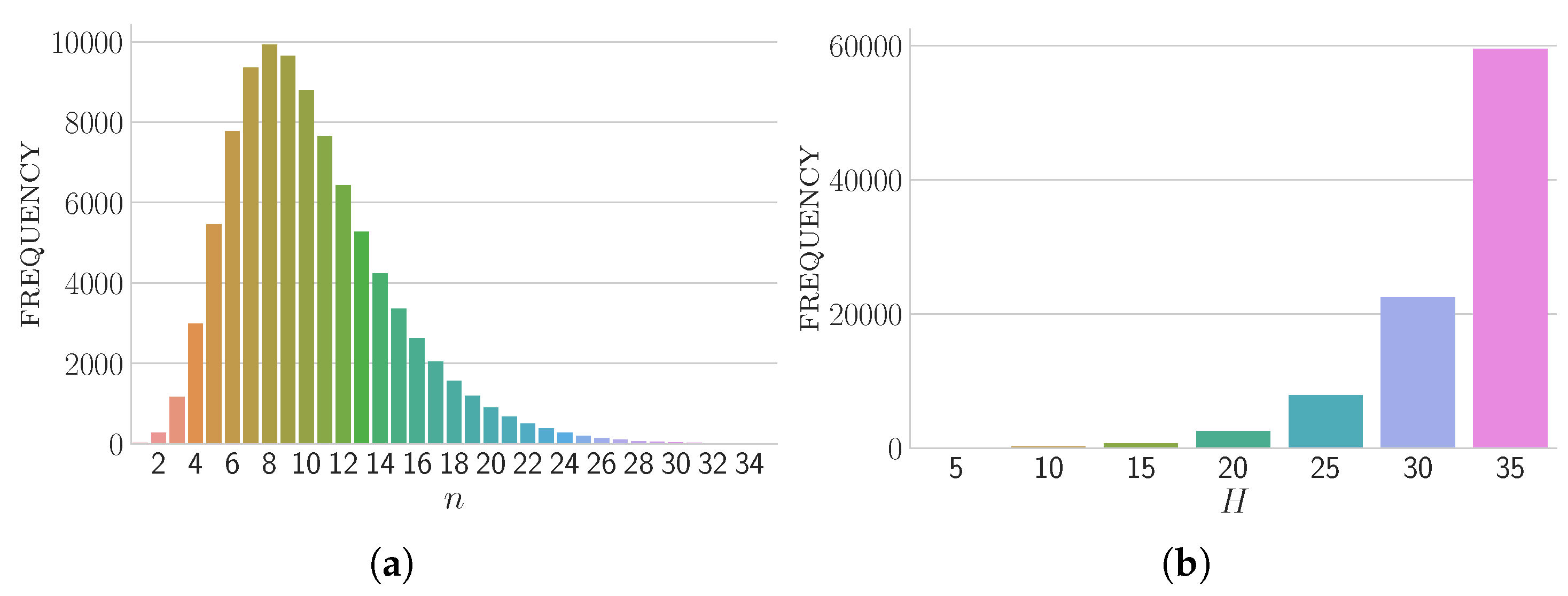
In the first set of experiments, parameter H was fixed and all possible input instances of n bamboos were considered whose growth rates sum up to H. Such instances were generated by considering, for a given H N , all integer partitions of H. Hence, clearly, the resulting n was in { 1 , 2 , , H } , where for n = 1 there was only one bamboo having growth rate equal to H while for n = H all bamboos had unitary growth rate (e.g., for H = 3 , we had instances [ 3 ] , [ 2 , 1 ] and [ 1 , 1 , 1 ] ). Note that, for H, values in the set { 5 , 10 , 15 , 20 , 25 , 30 , 35 } were selected. This choice was dictated by the fact that the number of integer partitions, and therefore instances to consider, grows very quickly as H increases and hence too large values of H induce a computationally prohibitive number of simulations. In particular, it is known that the number of integer partitions p ( k ) of a natural number k grows asymptotically as p ( k ) 1 4 k 3 e π 2 k 3 as k approaches infinity [30]. For instance, p(100) = 190,569,292 while p ( 1000 ) 2 . 41 · 10 31 . Figure 2b provides an overview of the total number of inputs considered in this experiment. However, the trend of the obtained results does not seem to be affected for H growing.
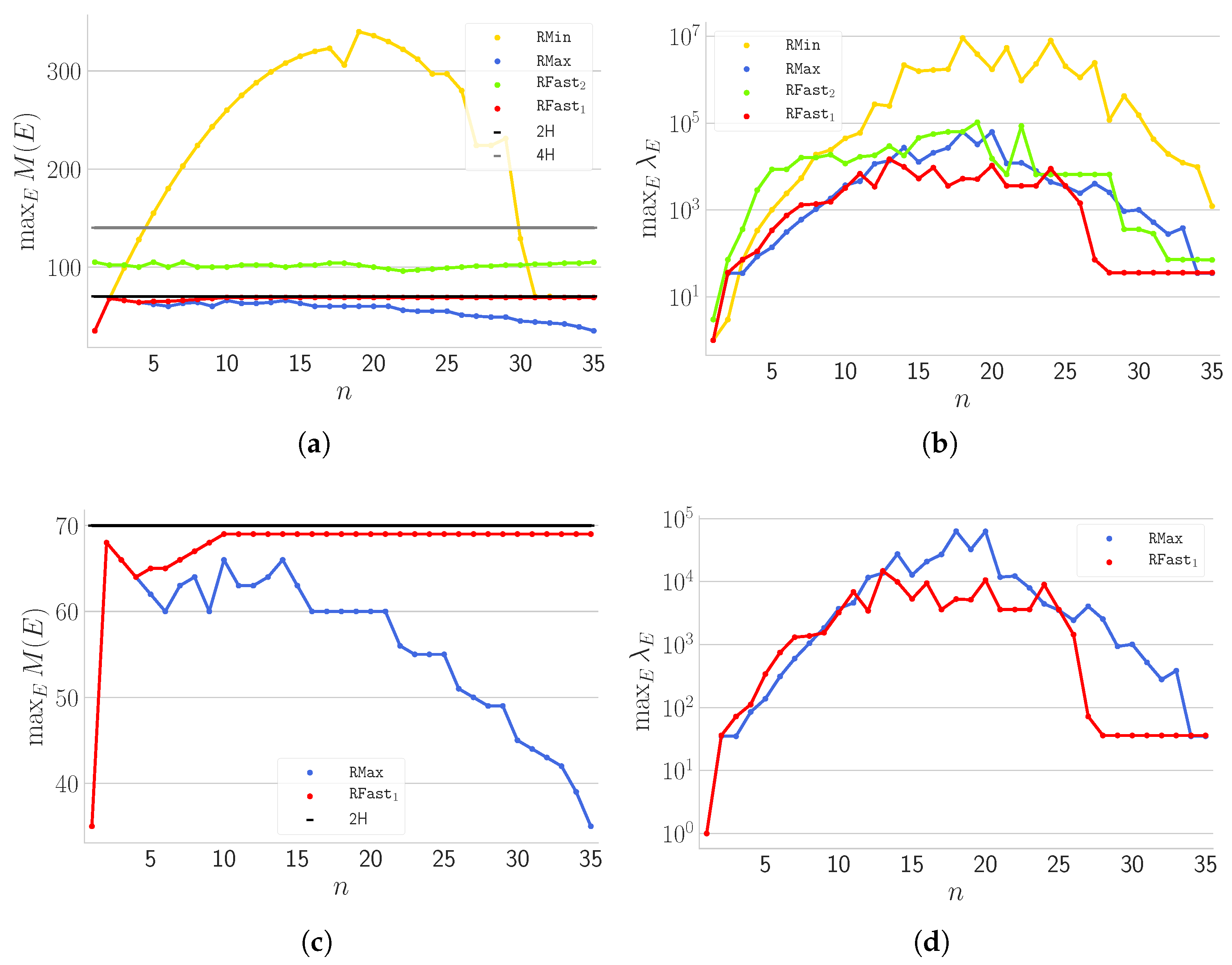
The results of the application of all the considered scheduling algorithms, on instances induced by the integer partitions H = 30 ( H = 35 , respectively) are shown in Figure 3 (Figure 4, respectively). Panels on the left side show how the maximum M ( E ) , obtained for all configurations and strategies, varies as a function of n (see Figure 3a,c and Figure 4a,c, respectively). Reference lines 2 H and 4 H are plotted to emphasise performance of the strategies in terms of M ( E ) . Panels on the right instead, instead, show how the achieved maximum value of λ E changes as a function of n, given that all strategies are guaranteed to stabilise into cycles.
Note that the maximum measured value is reported as it is possible to have many instances having the same n. Notice also that the results for H { 5 , 10 , 15 , 20 , 25 } lead to similar considerations with respect to those provided below, hence they have been omitted.
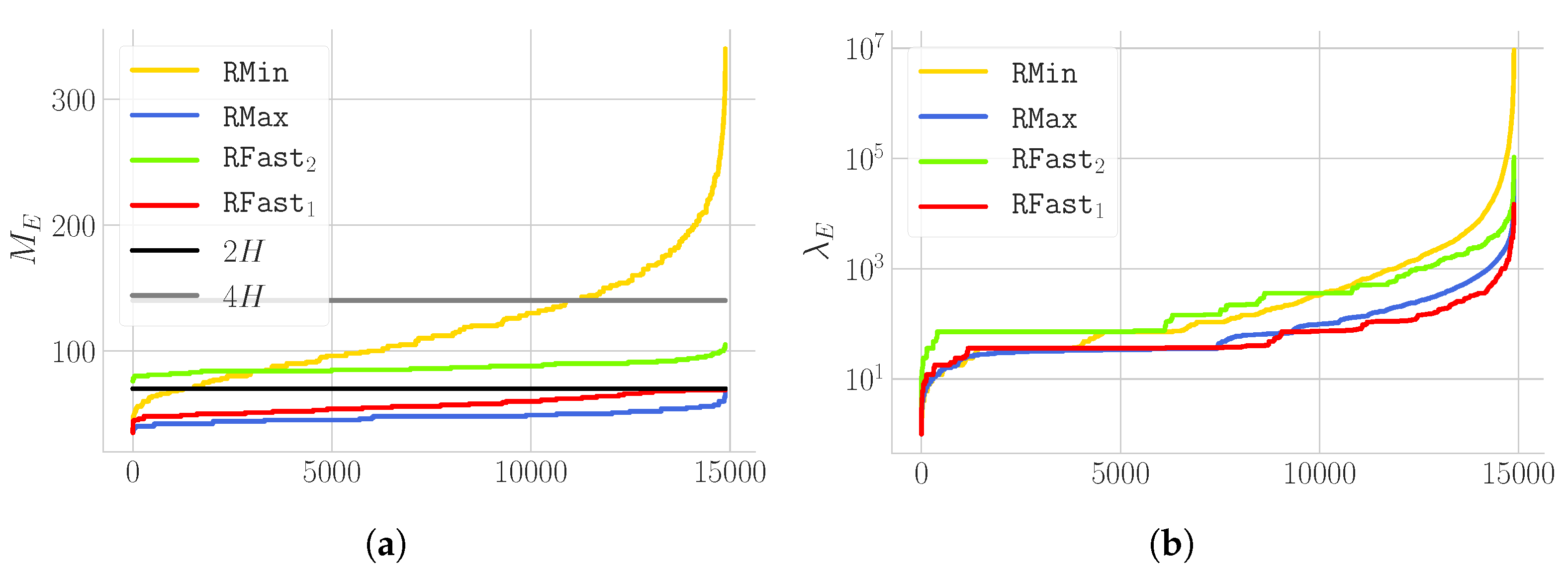
An alternative view of the results of the experiments for H = 35 is given in Figure 5 where it is shown how the obtained values of M ( E ) and λ E are distributed over the considered instances. In detail, each value on the x-axis in these diagrams simply represents one instance, to which the corresponding values of M ( E ) and λ E has been associated on the y-axis. Instances are sorted on the x-axis in non-decreasing order according to their values on the y-axis to highlight the amount of inputs providing a same value of M ( E ) and λ E . This information is condensed in Figure 4 where n is on the x-axis and the maximum values are plot only for each set of instances sharing the same value of n.
On the Maximum Height. The main and the most interesting outcome of this experiment is that, notwithstanding the O ( log n ) approximation factor [1], RMax exhibits properties of a 2-approximation, which can be observed as M ( E ) < 2 H . This supports the conjecture on the worst case approximation factor that has been proved so far being an over estimation of the true approximation upper bound. Another rather surprising evidence is that also RFast 1 is always below 2 H in terms of M ( E ) . This suggests that, for this strategy as well there could be a way to prove the worst case 2-approximation. However, RFast 1 seems to follow an asymptotic trend toward 2 H as n increases while a slowly decreasing trend for RMax when n increases can be observed.
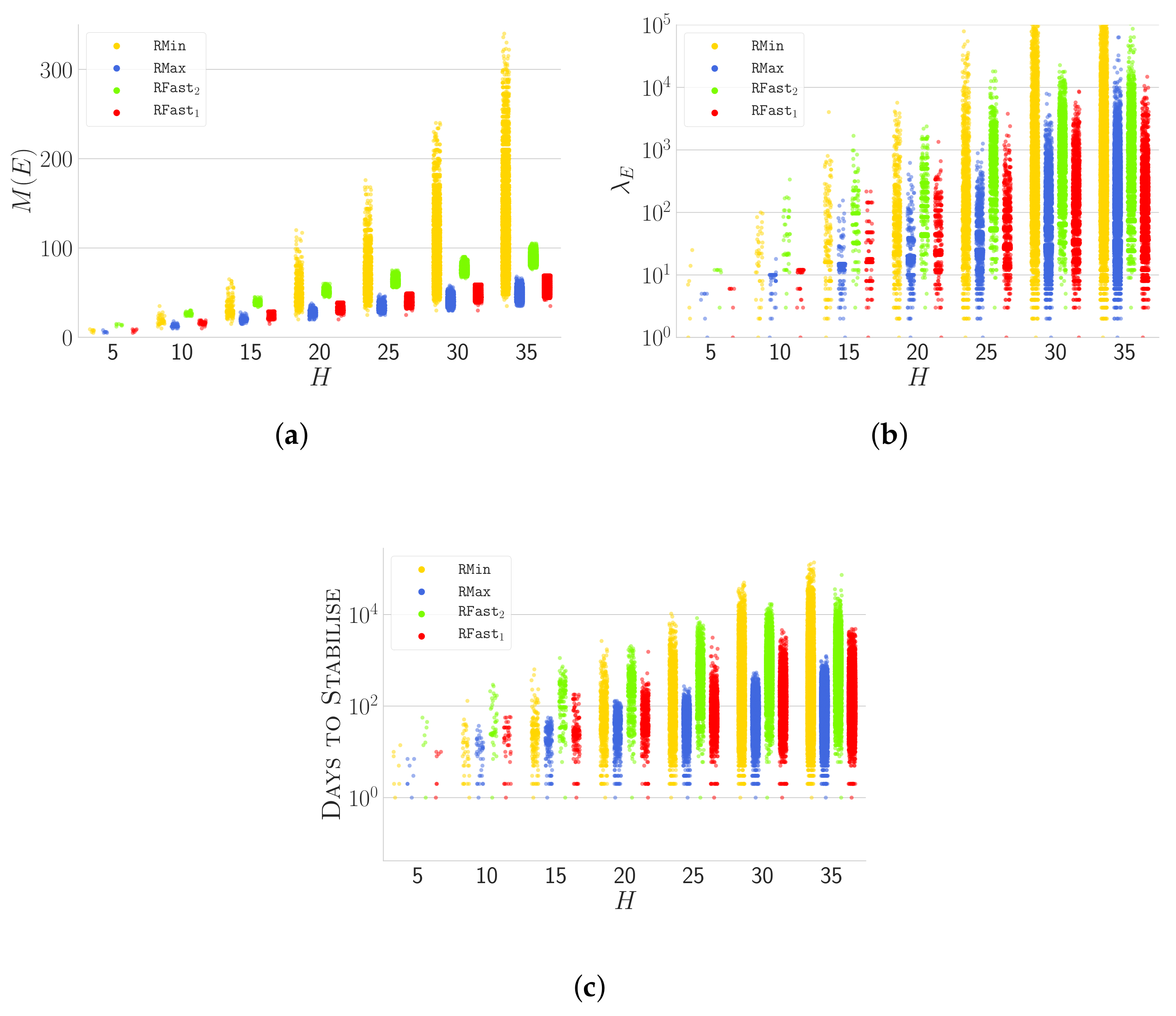
Concerning RFast 2 , from [1] it is known that M ( E ) is guaranteed to be below 4 H and this is confirmed by the performed tests. Nonetheless, it can be observed that M ( E ) is always above 2 H , which is expected since no actions are performed by RFast 2 when there are no bamboos having height above 2 H . However, the strategy exhibits a rather uniform behaviour, with M ( E ) stabilising toward threshold 3 H without ever overpassing it. This suggests that perhaps also the bound of 4 H guaranteed for RFast 2 is an overestimation of the true bound. Finally, regarding RMin , for low/high values of n (see Figure 3a and Figure 4a), it provides smaller values of M ( E ) with respect to RFast 2 , whereas for higher values of H its performance gets worse in the opposite sense. However, there no evidence of RMin exhibiting a constant approximation, with values of M ( E ) varying quite a lot with n. As a final remark, in Figure 5a, it can be observed that, for all strategies, values of maximum M ( E ) tend to have small variance among all instances having a same H, with curves assuming rather similar (flat) trends, and values always being very close to the average. The only exception is algorithm RMin , whose values of M ( E ) are quite different across instances having a same H. Moreover, RMax achieves values of M ( E ) that are far better than all other strategies, including RFast 1 , being below 2 H and, in some cases, below 3 2 H . This is even more evident in Figure 3c and Figure 4c where the focus is restricted on RMax and RFast 1 , i.e., on experiments where M ( E ) is observed to be always below 2 H . Finally, a global view supporting the conclusions with respect to the performance of the strategies in terms of M ( E ) is given in the scatterplot chart of Figure 6a where all obtained values of M ( E ) for all strategies and for all values of H are reported and compared.
On the Length of the Cycle. In Figure 3b and Figure 4b, the maximum λ E exhibited by all strategies is reported. Such values can be considered as proxy of the complexity of the periodic part of each execution, as higher values of λ E correspond to larger spaces of configurations that are explored by the strategies. This translates to higher variance in terms of height and volume, which can be seen as an undesired behaviour. Moreover, there might be also a relationship between such length and the quality of the provided factor of approximation, and it would be worth studying such relationship to define new bounds on this factor.
In more details, the data show a very big gap between the results obtained by RMax , RFast 1 , and those measured for RFast 2 , RMin , with the latter two tending to exhibit larger values with respect to the former two. In particular, as shown in Figure 4b, when n = 18 , RMin cyclic part takes around 10 7 steps, whereas the worst case for RFast 2 is obtained for n = 19 , with around 10 5 steps. Instead, RMax and RFast 1 behave rather differently with respect to other strategies, exhibiting lower values of λ E (e.g., up to around 3 orders of magnitude lower when n = 21 ).
This may be to more accurate arguments about changes in the volume of the garden, to be exploited in proofs of constant approximation. Different considerations can be done by observing Figure 5b. In particular, the largest values of λ E are achieved in the great majority of the cases by RFast 2 while RMax and RFast 1 result to be the best strategies also in this sense.

4.2. Fixed n Experimentation

In this section, the results of further experimentation are reported where parameter n is fixed and all possible instances with H n are considered, when H { 5 , 10 , 15 , 20 , 25 , 30 , 35 } . For example, when n = 15 , then H can assume values 15, 20 and 25. Instances are again chosen among all the integer partitions of specific values of H. Figure 2 provides an overview of the total number of inputs considered in this experiment, as a function of n and H, respectively.
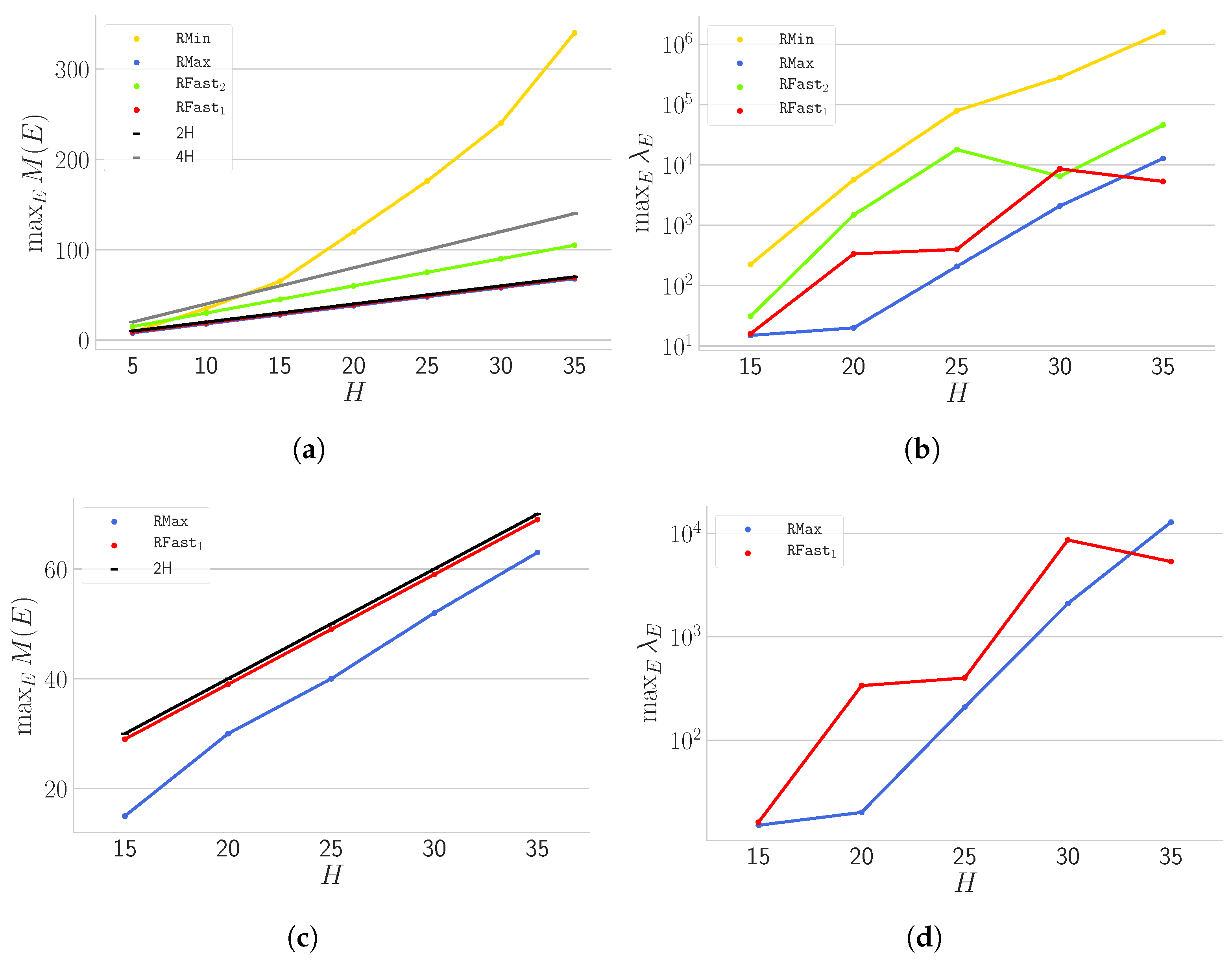
The results of this experiment are summarised in Figure 7 and Figure 8 where the results of application of all considered algorithms on instances with n = 10 and n = 15 , respectively, are shown. In particular, the maximum values of M ( E ) and λ E obtained by all strategies as a function of H are reported. Reference lines 2 H and 4 H are again used to highlight the quality in terms of M ( E ) obtained by the different algorithms. Note that graphs for other possible values of n (e.g., n = 20 ) are omitted since they lead to similar considerations with respect to those that follow.
On the Maximum Height. As already observed above, in this experiment, it was also possible to notice that RMax and RFast 1 exhibit values of M ( E ) that are always below 2 H (see Figure 7 and Figure 8). Moreover, again, RMax seems to be the best strategy, achieving values of maximum M ( E ) that are below 2 H and better than all other scheduling strategies, including RFast 1 . This is again more evident if the attention is restricted to RMax and RFast 1 only (see Figure 7). Furthermore, the experiments confirm also the theoretical bound of RFast 2 , with bamboos never exceeding 4 H . Moreover, all strategies exhibit a trend of M ( E ) with respect to H that looks linear, with the only exception of RMin , where the curve looks slightly super-linear.
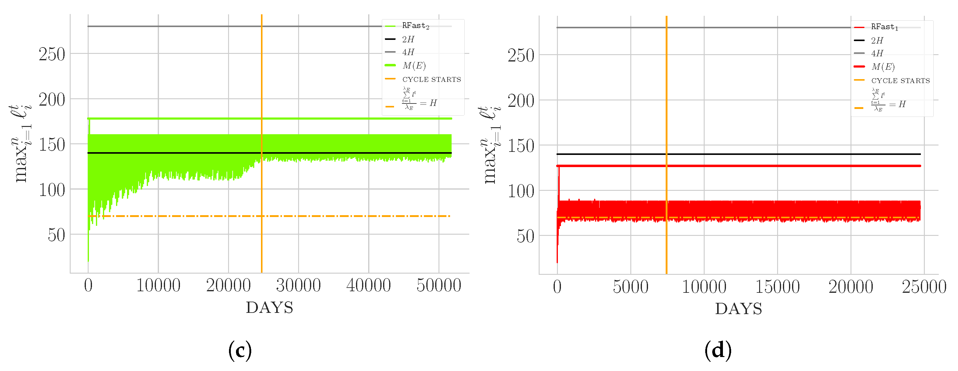
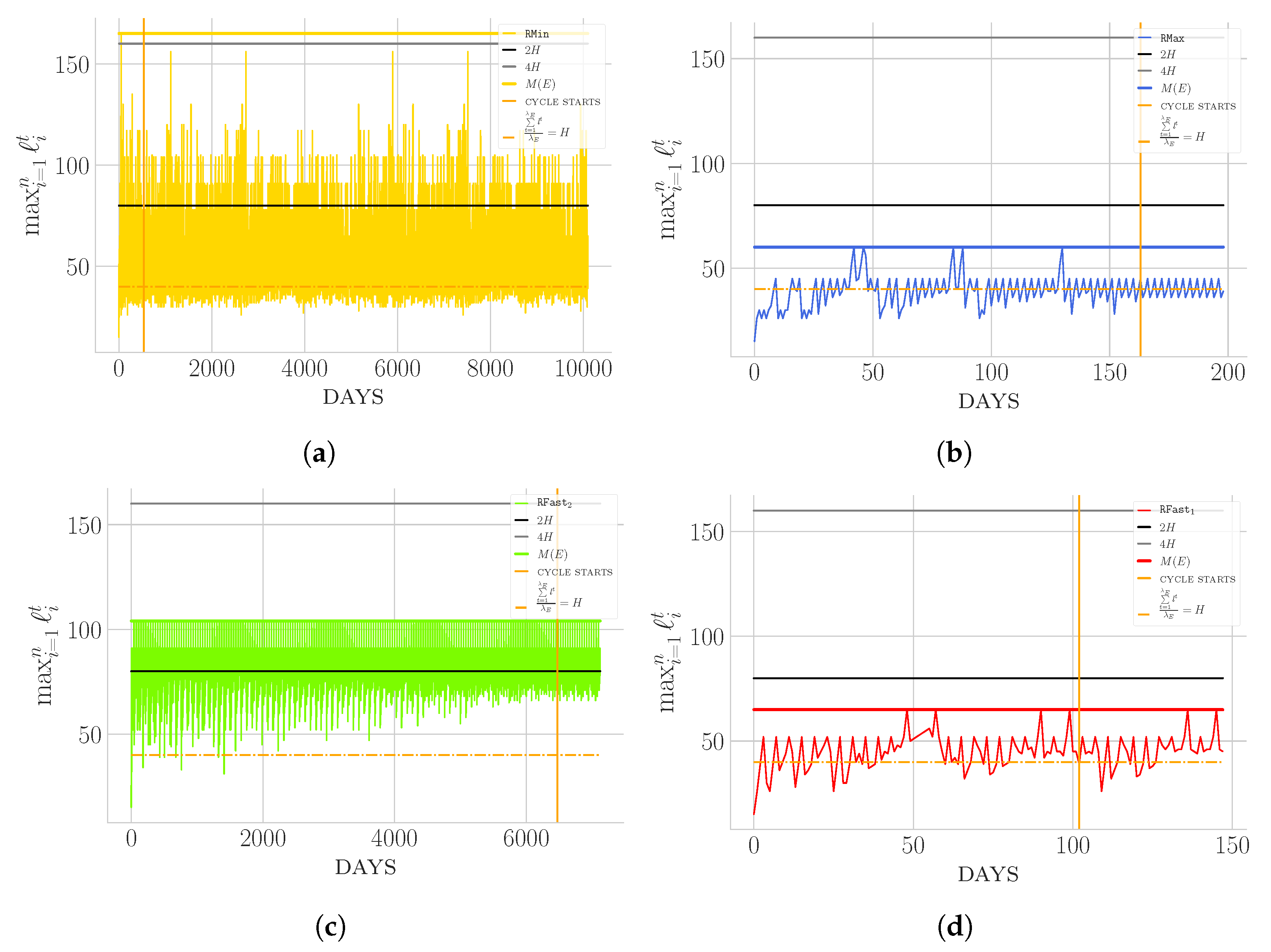
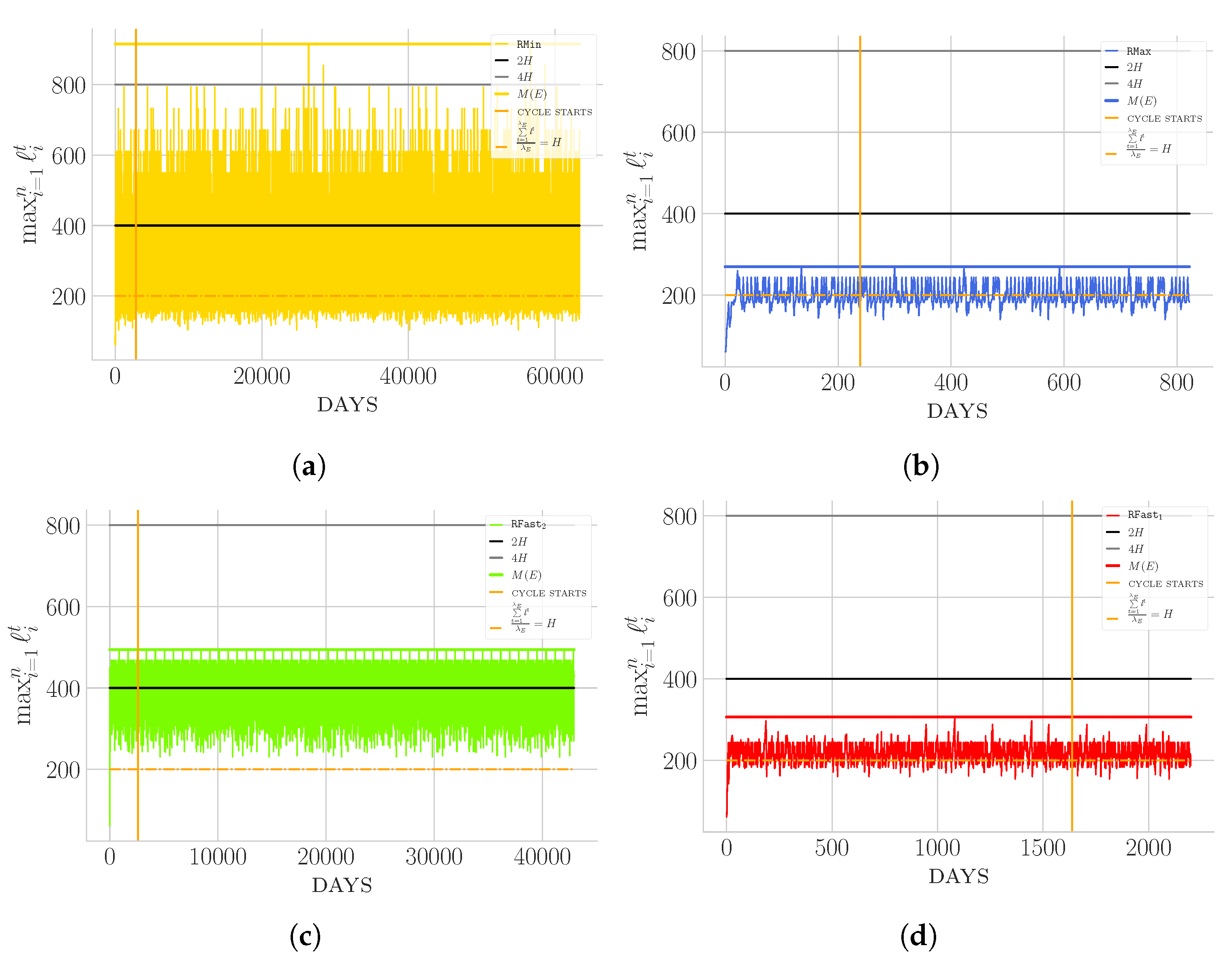
On the Length of the Cycle. In Figure 7b and Figure 8b, the maximum λ E obtained by all strategies in this setting is reported. The results confirm the trend observed in the case of fixed H. However, here it can be seen how RMin starts growing significantly faster for values of H that are greater than 20. Shortest cycles are obtained by RMax and ReduceFastest 1 . Still, the length of the cycle seems dependent on the way ties among bamboos are resolved (see Figure 7d). For the sake of completeness, in Figure 9, Figure 10, Figure 11 and Figure 12, the entire executions of the scheduling strategies are plotted on four sample instances whose size (i.e., n or H) is larger than all others considered in this paper, namely having:
  • n = 30 bamboos with H { 70 , 100 } ; and
  • n = 10 with H { 40 , 200 } .
This is done to highlight how each algorithm stabilises and how values of M ( E ) evolve both before the cyclic part starts (i.e., during the transient phase) and during such periodic part.
In particular, the height as a function of increasing values of days is shown and both the length of the periodic part and the number of days before each algorithm stabilises are highlighted. The data lead essentially to two major observations:
  • (i) Some strategies exhibit a very small variance in terms of height (e.g., RMax ) with respect to others (e.g., RMin ).
  • (ii) Some strategies (e.g., RMax ) are able to stabilise very quickly to a cycle, which is a clearly desirable behaviour in a stabilisation perspective. On top of that, they also exhibit a small λ E .
To support these observations, an aggregated view of all the measures of M ( E ) and λ E are shown, for all instances and strategies, as a function of H (see Figure 6a,b). Jointly, the distribution of the length of the transient phases, i.e., the number of days before each algorithm stabilises into the periodic part is reported (see Figure 6c). Furthermore, the panels suggest that the structure of the instances affects somehow the behaviour of the scheduling algorithms and the corresponding schedules. In more details, heterogeneous distributions of rates seem to be associated with higher values of M ( E ) , λ E and number of days before stabilisation while more evenly distributed rates tend to induce the opposite behavior. Finally, it is worth remarking on the successful verification that all the (priority) strategies investigated clearly do not violate the results of Section 3.1. Moreover, on the basis of the experimental results and in accordance to the special cases studied in Corollary 7, it is worth reporting again Conjecture 1 to emphasise and confirm the arisen intuition:
Conjecture 1.
Algorithm ReduceMax is 2-approximating for the BGT problem.
Further considerations for the other heuristics might be deducted, as for instance also ReduceFastest 1 seems to guarantee an approximation ratio of 2. However, as for ReduceFastest 2 , it relies on the ordering of the bamboos with respect to the growth rates.

5. Conclusions

The BGT problem has been investigated to establish whether constant approximation deterministic algorithms can be designed. A new class of scheduling strategies called priority schedulings have been defined and theoretical results on such methods have been provided. In particular, it has been proved that any priority scheduling eventually brings the system to perpetually repeated sequences of configurations. In addition, ReduceMax has been deeply analysed. This is a priority scheduling for which a conjecture of 2-approximation has been claimed. Extensive experimentation was conducted to confirm the intuitions and to show that ReduceMax outperforms any other known strategy, including the 4-approximation ReduceFastest 2 which, unlike ReduceMax , relies on the knowledge of an ordering on the rates. In terms of knowledge required by the cutting strategies, a research direction that surely deserves further investigation is that of considering the more realistic scenario where the input data are not entirely known, i.e., to tackle the problem from an online algorithms perspective. With respect to problem in its formulation, instead, it would be interesting to study variants of the model where, for example: (i) the aim is optimising other metrics of interest; and (ii) the gardener is allowed to perform different types of trimming operations. Finally, it would be worth studying how the results provided in this paper can translate to the continuous version of the problem [1].

Author Contributions

All authors have equally contributed to this work.

Funding

This work has been partially supported by the European project “Geospatial based Environment for Optimisation Systems Addressing Fire Emergencies” (GEO-SAFE), contract no. H2020-691161 and by the Italian National Group for Scientific Computation GNCS-INdAM.

Conflicts of Interest

The authors declare no conflict of interest.

References

  1. Gąsieniec, L.; Klasing, R.; Levcopoulos, C.; Lingas, A.; Min, J.; Radzik, T. Bamboo Garden Trimming Problem (Perpetual Maintenance of Machines with Different Attendance Urgency Factors). In SOFSEM 2017: Theory and Practice of Computer Science, Proceedings of the 43rd International Conference on Current Trends in Theory and Practice of Computer Science, Limerick, Ireland, 16–20 January 2017; Lecture Notes in Computer Science; Springer: Berlin, Germany, 2017; Volume 10139, pp. 229–240. [Google Scholar]
  2. Holte, R.; Mok, A.; Rosier, L.; Tulchinsky, I.; Varvel, D. The pinwheel: A real-time scheduling problem. In Proceedings of the 22nd Annual Hawaii International Conference on System Sciences, Kailua-Kona, HI, USA, 3–6 January 1989; Volume 2, pp. 693–702. [Google Scholar]
  3. Fishburn, P.C.; Lagarias, J.C. Pinwheel Scheduling: Achievable Densities. Algorithmica 2002, 34, 14–38. [Google Scholar] [CrossRef]
  4. Alshamrani, S.; Kowalski, D.R.; Gąsieniec, L. How Reduce Max Algorithm Behaves with Symptoms Appearance on Virtual Machines in Clouds. In Proceedings of the 2015 International Conference on Cloud Computing (ICCC), Riyadh, Saudi Arabia, 26–29 April 2015; pp. 1703–1710. [Google Scholar]
  5. Gąsieniec, L.; Klasing, R.; Martin, R.; Navarra, A.; Zhang, X. Fast periodic graph exploration with constant memory. J. Comput. Syst. Sci. 2008, 74, 802–822. [Google Scholar] [CrossRef]
  6. Kosowski, A.; Navarra, A. Graph Decomposition for Memoryless Periodic Exploration. Algorithmica 2012, 63, 26–38. [Google Scholar] [CrossRef]
  7. D’Emidio, M.; Di Stefano, G.; Frigioni, D.; Navarra, A. Characterizing the computational power of mobile robots on graphs and implications for the Euclidean plane. Inf. Comput 2018, 263, 57–74. [Google Scholar] [CrossRef]
  8. D’Emidio, M.; Frigioni, D.; Navarra, A. Explore and repair graphs with black holes using mobile entities. Theor. Comput. Sci. 2015, 605, 129–145. [Google Scholar] [CrossRef]
  9. Ntafos, S. On gallery watchmen in grids. Inf. Process. Lett. 1986, 23, 9–102. [Google Scholar] [CrossRef]
  10. Urrutia, J. Art gallery and illumination problems. In Handbook of Computational Geometry; Elsevier: Amsterdam, The Netherlands, 2000; pp. 973–1027. [Google Scholar]
  11. Collins, A.; Czyzowicz, J.; Gąsieniec, L.; Kosowski, A.; Kranakis, E.; Krizanc, D.; Martin, R.; Morales Ponce, O. Optimal Patrolling of Fragmented Boundaries. In Proceedings of the 25th Annual ACM Symposium on Parallelism in Algorithms and Architectures, Montréal, QC, Canada, 23–25 July 2013; ACM: New York, NY, USA, 2013; pp. 241–250. [Google Scholar]
  12. Czyzowicz, J.; Gąsieniec, L.; Kosowski, A.; Kranakis, E. Boundary Patrolling by Mobile Agents with Distinct Maximal Speeds. In Algorithms—ESA 2011, Proceedings of the 19th Annual European Symposium, Saarbrücken, Germany, 5–9 September 2011; Lecture Notes in Computer Science; Springer: Berlin, Germany, 2011; Volume 6942, pp. 701–712. [Google Scholar]
  13. Chuangpishit, H.; Czyzowicz, J.; Gąsieniec, L.; Georgiou, K.; Jurdzinski, T.; Kranakis, E. Patrolling a Path Connecting a Set of Points with Unbalanced Frequencies of Visits. In SOFSEM 2018: Theory and Practice of Computer Science, Proceedings of the 44th International Conference on Current Trends in Theory and Practice of Computer Science, Krems, Austria, 29 January–2 February 2018; Lecture Notes in Computer Science; Springer: Berlin, Germany, 2018; Volume 10706, pp. 367–380. [Google Scholar]
  14. Serafini, P.; Ukovich, W. A Mathematical Model for Periodic Scheduling Problems. SIAM J. Discret. Math. 1989, 2, 550–581. [Google Scholar] [CrossRef]
  15. Chan, M.Y.; Chin, F.Y.L. General schedulers for the pinwheel problem based on double-integer reduction. IEEE Trans. Comput. 1992, 41, 755–768. [Google Scholar] [CrossRef]
  16. Chan, M.Y.; Chin, F.Y.L. Schedulers for larger classes of pinwheel instances. Algorithmica 1993, 9, 425–462. [Google Scholar] [CrossRef]
  17. Hsueh, C.; Lin, K. An Optimal Pinwheel Scheduler Using the Single-number Reduction Technique. In Proceedings of the 17th IEEE Real-Time Systems Symposium, Washington, DC, USA, 4–6 December 1996; pp. 196–205. [Google Scholar]
  18. Holte, R.; Rosier, L.; Tulchinsky, I.; Varvel, D. Pinwheel scheduling with two distinct numbers. Theor. Comput. Sci. 1992, 100, 105–135. [Google Scholar] [CrossRef]
  19. Lin, S.S.; Lin, K.J. A Pinwheel Scheduler for Three Distinct Numbers with a Tight Schedulability Bound. Algorithmica 1997, 19, 411–426. [Google Scholar] [CrossRef]
  20. Romer, T.H.; Rosier, L.E. An algorithm reminiscent of euclidean-gcd for computing a function related to pinwheel scheduling. Algorithmica 1997, 17, 1–10. [Google Scholar] [CrossRef]
  21. Baruah, S.K.; Lin, S.-S. Pfair scheduling of generalized pinwheel task systems. IEEE Trans. Comput. 1998, 47, 812–816. [Google Scholar] [CrossRef]
  22. Baruah, S.K.; Cohen, N.K.; Plaxton, C.G.; Varvel, D.A. Proportionate progress: A notion of fairness in resource allocation. Algorithmica 1996, 15, 600–625. [Google Scholar] [CrossRef]
  23. Mok, A.; Rosier, L.; Tulchinski, I.; Varvel, D. Algorithms and complexity of the periodic maintenance problem. Microprocess. Microprogram. 1989, 27, 657–664. [Google Scholar] [CrossRef]
  24. Anily, S.; Glass, C.A.; Hassin, R. The scheduling of maintenance service. Discret. Appl. Math. 1998, 82, 27–42. [Google Scholar] [CrossRef]
  25. Anily, S.; Glass, C.A.; Hassin, R. Scheduling maintenance services to three machines. Ann. Oper. Res. 1999, 86, 375–391. [Google Scholar] [CrossRef]
  26. Bender, M.A.; Fekete, S.P.; Kröller, A.; Mitchell, J.S.B.; Liberatore, V.; Polishchuk, V.; Suomela, J. The Minimum Backlog Problem. Theor. Comput. Sci. 2015, 605, 51–61. [Google Scholar] [CrossRef]
  27. Bodlaender, M.H.L.; Hurkens, C.A.J.; Kusters, V.J.J.; Staals, F.; Woeginger, G.J.; Zantema, H. Cinderella versus the Wicked Stepmother. In TCS 2012: Theoretical Computer Science, Proceedings of the IFIP Theoretical Computer Science Conference, Amsterdam, The Netherlands, 26–28 September 2012; Lecture Notes in Computer Science; Springer: Berlin, Germany, 2012; Volume 6942, pp. 57–71. [Google Scholar]
  28. Chrobak, M.; Csirik, J.; Imreh, C.; Noga, J.; Sgall, J.; Woeginger, G.J. The Buffer Minimization Problem for Multiprocessor Scheduling with Conflicts. In Automata, Languages and Programming, Proceedings of the 28th International Colloquium on Automata, Languages, and Programming, Crete, Greece, 8–12 July 2001; Lecture Notes in Computer Science; Springer: Berlin, Germany, 2001; Volume 2076, pp. 862–874. [Google Scholar]
  29. D’Emidio, M.; Di Stefano, G.; Navarra, A. Priority Scheduling in the Bamboo Garden Trimming Problem. In SOFSEM 2019: Theory and Practice of Computer Science, Proceedings of the 45th International Conference on Current Trends in Theory and Practice of Computer Science, Nový Smokovec, Slovakia, 27–30 January 2019; Lecture Notes in Computer Science; Springer: Berlin, Germany, 2019; Volume 11376, pp. 136–149. [Google Scholar]
  30. Hardy, G.H.; Ramanujan, S. Asymptotic formulas in combinatorial analysis. Proc. Lond. Math. Soc. 1918, 17, 75–115. [Google Scholar] [CrossRef]
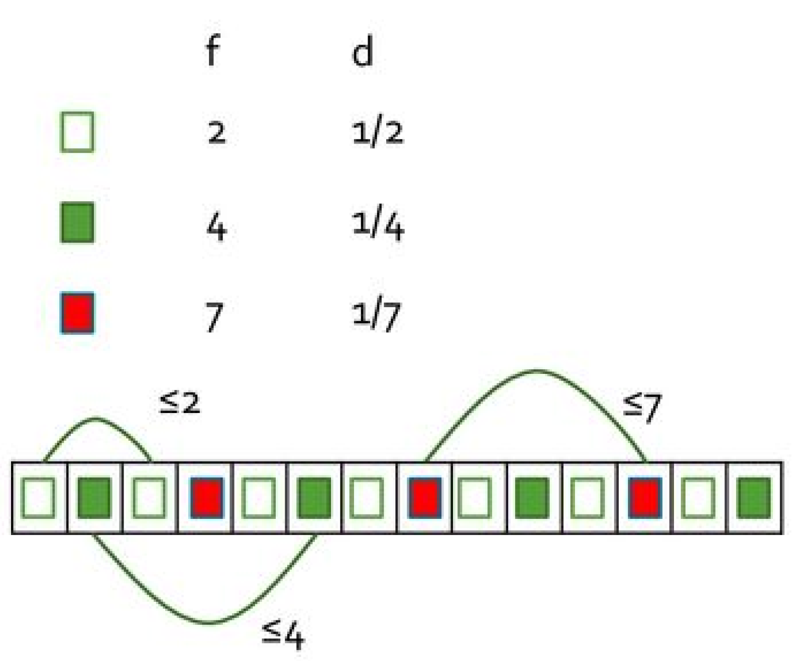
Figure 1. An example of input instance for the Pinwheel problem where V = ( 2 , 4 , 7 ) and hence D = 1 / 2 + 1 / 4 + 1 / 7 0 . 89 .
Algorithms 12 00074 g001
Figure 2. (a) Distribution of instances with respect to n for all partitions of integer H { 5 , 10 , 15 , 20 , 25 , 30 , 35 } ; and (b) distribution of instances with respect to H for all partitions of integer H { 5 , 10 , 15 , 20 , 25 , 30 , 35 } .
Algorithms 12 00074 g002
Figure 3. Experiments conducted on all possible ordered instances obtained by setting H = 30 and hence considering n varying in { 1 , 2 , , 30 } . Panels (a,c) refer to maximum M ( E ) , whereas panels (b,d) refer to maximum λ E . Panels (c,d) show strategies that, experimentally, exhibit 2-approximation.
Algorithms 12 00074 g003
Figure 4. Experiments conducted on all possible ordered instances obtained by setting H = 35 and hence considering n varying in { 1 , 2 , , 35 } . Panels (a,c) refer to maximum M ( E ) , whereas panels (b,d) refer to maximum λ E . Panels (c,d) show strategies that, experimentally, exhibit 2-approximation.
Algorithms 12 00074 g004
Figure 5. Distribution of values of: M ( E ) (a); and λ E (b) exhibited by all algorithms on instances induced by all partitions of H = 35 . Instances are sorted by non-decreasing values of: M ( E ) (a); and λ E (b). To magnify the differences, the y-axis in (b) is log-scaled.
Algorithms 12 00074 g005
Figure 6. Distribution of values of: M ( E ) (a); λ E (b); and number of days before stabilisation (c) as a function of H, for all considered strategies and instances.
Algorithms 12 00074 g006
Figure 7. How maximum M ( E ) (a,c) and maximum λ E (b,d) change as a function of H when instances are induced by all partitions of H { 10 , 15 , 20 , 25 , 30 , 35 } having cardinality n = 10 . Panels (c,d) show strategies that, experimentally, exhibit 2-approximation.
Algorithms 12 00074 g007
Figure 8. How maximum M ( E ) (a) and maximum λ E (b) change as a function of H when instances are induced by all partitions of H { 15 , 20 , 25 , 30 , 35 } having cardinality n = 15 . Panels (c,d) show strategies that, experimentally, exhibit 2-approximation.
Algorithms 12 00074 g008
Figure 9. Snapshot of the evolution of maximum heights when strategies: RMin (a); RMax (b); RFast 2 (c); and RFast 1 (d) are applied on an instance having n = 30 and H = 70 . (in details, structured as follows [ 20 ; 11 ; 8 ; 5 ; 1 ; 1 ; 1 ; 1 ; 1 ; 1 ; 1 ; 1 ; 1 ; 1 ; 1 ; 1 ; 1 ; 1 ; 1 ; 1 ; 1 ; 1 ; 1 ; 1 ; 1 ; 1 ; 1 ; 1 ; 1 ; 1 ] ). On the x-axis the consecutive days are reported while on the y-axis the maximum height on the corresponding day is plot. The vertical line shows the beginning of the periodic phase while the horizontal lines show, respectively, ( t = 1 λ E l t ) / λ E (i.e., H), 2 H , 4 H , and M ( E ) over the entire execution.
Algorithms 12 00074 g009aAlgorithms 12 00074 g009b
Figure 10. Snapshot of the evolution of maximum heights when strategies: RMin (a); RMax (b); RFast 2 (c); and RFast 1 (d) are applied on an instance having n = 30 and H = 100 (in details, structured as follows [ 70 ; 2 ; 1 ; 1 ; 1 ; 1 ; 1 ; 1 ; 1 ; 1 ; 1 ; 1 ; 1 ; 1 ; 1 ; 1 ; 1 ; 1 ; 1 ; 1 ; 1 ; 1 ; 1 ; 1 ; 1 ; 1 ; 1 ; 1 ; 1 ; 1 ] ). Data are plotted as in Figure 9.
Algorithms 12 00074 g010
Figure 11. Snapshot of the evolution of maximum heights when strategies: RMin (a); RMax (b); RFast 2 (c); and RFast 1 (d) are applied on an instance having n = 10 and H = 40 (in details, structured as follows [ 15 ; 13 ; 4 ; 2 ; 1 ; 1 ; 1 ; 1 ; 1 ; 1 ] ). Data are plotted as in Figure 9.
Algorithms 12 00074 g011
Figure 12. Snapshot of the evolution of maximum heights when strategies: RMin (a); RMax (b); RFast 2 (c); and RFast 1 (d) are applied on an instance having n = 10 and H = 200 (in details, structured as follows [ 61 ; 30 ; 27 ; 26 ; 13 ; 11 ; 10 ; 10 ; 9 ; 3 ] ). Data are plotted as in Figure 9.
Algorithms 12 00074 g012