Convex-Hull Algorithms: Implementation, Testing, and Experimentation

Abstract

From a broad perspective, we study issues related to implementation, testing, and experimentation in the context of geometric algorithms. Our focus is on the effect of quality of implementation on experimental results. More concisely, we study algorithms that compute convex hulls for a multiset of points in the plane. We introduce several improvements to the implementations of the studied algorithms: plane-sweep, torch, quickhull, and throw-away. With a new set of space-efficient implementations, the experimental results—in the integer-arithmetic setting—are different from those of earlier studies. From this, we conclude that utmost care is needed when doing experiments and when trying to draw solid conclusions upon them.

1. Introduction

In physics, the term observer effect is used to refer to the fact that simply observing a phenomenon necessarily changes that phenomenon. A similar effect arises in computer science when comparing different algorithms—one has to implement them and make measurements on the performance of the developed implementations. In an ideal situation, one would eliminate the bias caused by quality of implementation and limit the uncertainty caused by inaccurate measurements ([1], Chapter 14). In practice, this is difficult. This work is part of our research program “quality of implementation” where we look closely at the programs used in some recent algorithm-engineering studies. In particular, we want to remind our colleagues of the fact that, due to the programming details, some experiments do not tell the whole story and that the quality of implementation does matter.

More specifically, we investigate the efficiency of algorithms that solve the convex-hull problem in the two-dimensional Euclidean space. As our starting point, we used a recent article by Gomes [2] where a variation of the plane-sweep algorithm by Andrew [3] was presented, analysed, and experimentally compared to several other well-known algorithms. The algorithm was named torch (total-order convex-hull). The source code used in the experiments was released in an electronic appendix [4].

As in any experimental work, the experiments must be verifiable and reproducible. In the abstract of the paper [2], Gomes claimed that torch is (1) “much faster” than its competitors (2) “without penalties in memory space”. We set a simple goal for this study: Try to reproduce these results. Unfortunately, we must directly report that we failed in this mission for several reasons:

• The algorithm—as it was presented in [2]—was incorrect.
• The implementation given in [4] was not reliable—calculations could overflow and degenerate inputs were not handled correctly.
• The implementation required too much memory to be used when the size of the problem reached that of the main memory of the computer.
• The source code of the competing implementations was not made publicly available so we had to implement them ourselves.
• Not enough details were provided on the experiments so that we could reproduce them.

We built this paper around the same algorithms as Gomes [2]: rotational-sweep (Graham’s scan) [5], gift-wrapping (Jarvis’ march) [6], Chan’s output-sensitive algorithm [7], plane-sweep (Andrew’s monotone-chain algorithm) [3], torch [2], and quickhull [8,9,10]. Moreover, we examined some heuristics (poles-first [11] and throw-away [12]) that are often used as a preprocessing step to speed up the standard algorithms.

As advised in ([13], Section 2.3), we divided this study into two parts: (1) In a less formal pilot study, our goal was to eliminate unpromising avenues of research. (2) In a more carefully designed workhorse study, we compared the performance of the most serious competitors. In the remaining part of the paper, we describe how we implemented and tested the convex-hull algorithms that rose above the others: plane-sweep, torch, quickhull, and throw-away. We also discuss why the other alternatives mentioned above are not competitive. In particular, we go a bit deeper into some implementation details revealed by a careful code analysis. Finally, we present the results of our workhorse experiments and a totally new set of conclusions.

The contributions of this work can be summarized as follows.

• We describe a simple way of making the implementations of convex-hull algorithms robust.
• We identify an error in the original version of torch and propose a corrected, in-place version.
• We prove that, when the coordinates of the n input points are integers drawn from a bounded universe of size U, quickhull runs in $O\left(n\lg U\right)$ worst-case time. We also explain how its worst-case performance can be reduced to $O\left(n\lg n\right)$—we call this variant introhull.
• We implement six convex-hull algorithms—plane-sweep, torch, quickhull, poles-first, throw-away, and introhull—and show that these implementations are space-efficient and time-efficient, both in theory and practice.
• We introduce a test framework that can be used to make the programs computing convex hulls self-testing.
• We compare the performance of four space-efficient convex-hull algorithms—plane-sweep, torch, quickhull, and throw-away—in the integer-arithmetic setting.

2. Preliminaries

We begin with some basics that are important for the whole study: (1) We define the terms used formally, (2) we describe the environment where all pilot and workhorse experiments were carried out, and (3) we discuss the robustness issue that is relevant for many geometric algorithms.

2.1. Definitions

Recall that in the two-dimensional convex-hull problem we are given a multiset S of points, where each point p is specified by its Cartesian coordinates $(p.x,p.y)$, and the task is to compute the convex hull $\mathcal{H}\left(S\right)$ of S which is the boundary of the smallest convex set enclosing all the points of S. More precisely, the goal is to find the smallest set—in cardinality—of vertices describing the convex hull, i.e., the output is a convex polygon P covering all the points of S. In particular, the set of vertices in P is a subset of the points in S. A normal requirement is that in the output the vertices are reported in the order in which they appear when traversing around the convex hull. Throughout the paper, we use n to denote the number of points in the input S and h the number of vertices in the output P.

A point q of a convex set X is said to be an extreme point if no two other points p and r exist in X such that q lies on the line segment $\overline{pr}$. So, the vertices of P describing the convex hull $\mathcal{H}\left(S\right)$ are precisely the extreme points of the smallest convex set enclosing the points of S.

Let S be a multiset of points. Of these points, a point p dominates another point q in the north-east direction if $p.x>q.x$ and $p.y>q.y$. Since the requirement is to be strictly larger in both x and y, then for a pair of points as $(1,1)$ and $(1,2)$, we have that neither of them dominate the other in the north-east direction. A point p is dominant in the north-east direction if it is not dominated in this particular direction by any other point in S. That is, the first quadrant centred at p has no other point in it. Analogous definitions can be made for the south-east, south-west, and north-west directions. A point is said to be maximal among the points in S if it is dominant in one of the four directions. Clearly, every extreme point is maximal (for a proof, see [14]), but the opposite is not necessarily true.

An algorithm operates in place if the input is given in a sequence of size n and, in addition to this, it uses $O\left(1\right)$ words of memory. An in-place convex-hull algorithm (see, for example, [15]) partitions the input into two parts: (1) The first part contains all the extreme points in clockwise or counterclockwise order of their appearance on P and (2) the second part contains all the remaining points that are inside or on the periphery of P. Further, an algorithm operates in situ if it uses $O\left(\lg n\right)$ words of extra memory. For example, quicksort [16] is an in-situ algorithm if it is implemented recursively such that the smaller subproblem is always solved first.

2.2. Test Environment

The experiments to be discussed were run on two computers: one running Linux and the other running Windows. Both computers could be characterized as standard laptops that one can buy from any well-stocked computer store. A summary of the test environments is given in

Table 1. Hardware and software in use: (a) Linux computer, (b) Windows computer.

(a)

Processor. Intel${}^{\circledR }$ Core™ i7-6600U CPU @ 2.6 GHz (turbo-boost up to 3.6 GHz)—4 cores

Word size. 64 bits

First-level data cache. 8-way set-associative, 64 sets, $4\times 32$ KB

First-level instruction cache. 8-way set-associative, 64 sets, $4\times 32$ KB

Second-level cache. 4-way set-associative, 1 024 sets, 256 KB

Third-level cache. 16-way set-associative, 4 096 sets, 4.096 MB

Main memory. 8.038 GB

Operating system. Ubuntu 17.10

Kernel. Linux 4.13.0-16-generic

Compiler. g++ 7.2.0

Compiler options.-O3 -std=c++17 -x c++ -Wall -Wextra -fconcepts

(b)

Processor. Intel${}^{\circledR }$ Core™ i7-4700MQ CPU @ 2.40 GHz—4 cores and 8 logic processors

Word size. 64 bits

First-level data cache. 8-way set-associative, $4\times 32$ KB

First-level instruction cache. 8-way set-associative, $4\times 32$ KB

Second-level cache. 4-way set-associative, $4\times 256$ KB

Third-level cache. 12-way set-associative, 6 MB

Main memory. DDR3, 8 GB, DRAM frequency 800 MHz

Operating system. Microsoft Windows 10 Home 10.0.15063

Compiler. Microsoft Visual Studio 2017

Compiler options./Ox /Ob2 /Oi /Ot /std:c++17

. Although both computers had four cores, the experiments were run on a single core.

As the input for the programs, we used three types of data:

• Square data set. The coordinates of the points were random integers uniformly distributed over the interval $〚-2^{31}..2^{31}⦈$ (i.e., random ints). The expected size of the output is $O\left(\lg n\right)$ [14].
• Disc data set. As above, the coordinates of the points were random ints, but only the points inside the circle centred at the origin $(0,0)$ with the radius $2^{31}-1$ were accepted to the input collection. In this case, the expected size of the output is $O\left(n^{1/3}\right)$.
• Bell data set. The points were drawn according to a two-dimensional normal distribution by rounding each coordinate to the nearest integer value (of type int). The mean value of the distribution was 0 and the standard deviation $r/(2+{\log }_e\left(n\right))$ where $r=2^{31}-1$. For this data set, the expected size of the output is $O\left(\sqrt{\lg n}\right)$.

All our programs used the same point class template that took the type of the coordinates as its template parameter. The implementation of this class was straightforward: It had two public data members x and y, it had a default constructor and a parameterized constructor, and it supported the operations $\left\{==,\ne ,<,>\right\}$ for any pair of points.

None of the considered algorithms use random-access capabilities to a large extent. Therefore, we did not expect to see any significant cache effects in our experiments. Based on the memory configuration of the test computers, we wanted to check what happened when the problem instances became bigger than the capacity of different memory levels. In particular, it seemed not to be necessary to plot detailed curves of the running times.

The points were stored in an array. We report the test results for five values of n: $2^{10}$, $2^{15}$, $2^{20}$, $2^{25}$, and $2^{30}$. Observe that for the largest test case, there could be at most one array of $2^{30}$ points in the internal memory of the Linux computer, while the Windows computer could not handle that.

Be aware that the reported measurement results are scaled: For every performance indicator, if X is the observed number, we report $X/n$. That is, a constant means linear performance. To avoid problems with inadequate clock precision and pseudo-random number generation, a test for $n=2^i$ was repeated $\lceil 2^{27}/2^i\rceil$ times; each repetition was done with a new input array. The input arrays were pre-generated and statistically independent.

2.3. Robustness

In Gomes’ experiments [2], the coordinates of the points were floating-point numbers. It is well-known that the use of the floating-point arithmetic in the implementation of the basic geometric primitives may lead to disasters (for some classroom examples—one being the computation of the convex hulls in the plane, we refer to [17]). Therefore, it was somewhat surprising that the robustness issue was not discussed at all. Given the floating-point setting, the programs used in Gomes’ study [2], as well in some other experimental studies (see, for instance, [18,19]), are only able to compute an uncontrolled approximation of the convex hull. The output polygon may not even be convex, it may miss some of the convex-hull vertices, and it may contain some interior points—in an uncontrolled away.

The orientation test is a basic primitive that is used in many geometric algorithms. It takes three points p, q, and r, and tells whether there is a left turn, right turn, or neither of these at q when moving from p to r via q. This primitive can be seen as a special cross-product computation, and it is a known improvement used to avoid trigonometric functions and division.

Recall that an overflow means that the result of an arithmetic operation is too large or too small to be correctly represented in the target variable ([20], Section 2-13). In our experiments we rely on the exact-arithmetic paradigm. The coordinates of the points are assumed to be integers of fixed width, and intermediate calculations are carried out with integers of higher precision so that all overflows are avoided. When computing convex hulls in the plane, it is easy to predict the maximum precision needed in the intermediate calculations. A construction of a signed value from an unsigned one may increase the length of the representation by one bit, every addition or subtraction may increase the needed precision by one bit, and every multiplication at most doubles the needed precision.

For points $p=(p.x,p.y)$, $q=(q.x,q.y)$, and $r=(r.x,r.y)$, we treat their cross product as a single number $(q.x-p.x)(r.y-p.y)-(r.x-p.x)(q.y-p.y)$. If the cross product is positive, there is a left turn at q when moving from p to r via q. If the cross product is negative, there is a right turn. Additionally, if it is 0, the points are collinear. The cross product measures the (signed) area of the parallelogram spanned by the oriented line segments $\overrightarrow{pq}$ and $\overrightarrow{pr}$. So the cross product can also be used to determine which point r is farthest from the line segment $\overline{pq}$ (above or below).

Let us consider how the left-turn orientation predicate can be coded in C++. The code for the right-turn, no-turn, and signed-area calculations is similar. Using the off-the-shelf tools available at the CPH MPL [21] and the CPH STL [22], the C++ code for computing the left-turn predicate is shown in Figure 1. If the width of the original coordinates is w bits, with (2w + 4)-bit intermediate precision we can be sure that no overflows happen—and the computed answer is correct. There are many other—more advanced—methods to make this computation robust (for a survey, we refer to [23]).

One left-turn test involves two multiplications, four subtractions, six constructor calls, and one comparison. When the numbers are wider than any of the built-in integers, we have to operate on double-word (cphstl::bbb$\mathbb{Z}$<68>) or triple-word integers (cphstl::bbb$\mathbb{Z}$<132>). This makes the arithmetic operations even more costly. Hence, the goal to reduce the number of times the geometric primitives are to be executed is well motivated.

3. Pilot Experiments

A normal advice given in most textbooks on algorithm engineering is that “it is essential to identify an appropriate baseline” for the experiments (the quotation is from ([1], Chapter 14)). The main outcome of our pilot experiments—to be discussed next—was that we can exclude rotational-sweep, gift-wrapping, and Chan’s output-sensitive algorithm from further consideration. None of them were competitive. Hence, we can follow the good practice “not to overload the experimental results with unnecessary curves” [24].

3.1. Rotational Sweep

The rotational-sweep algorithm due to Graham [5] is historically important; it was the first algorithm that could compute the convex hull of n points in $O\left(n\lg n\right)$ worst-case time. This algorithm works as follows: (1) Find a point o that is on the convex hull (e.g., a point that is lexicographically the smallest). (2) Sort all the points around o lexicographically by polar angle and distance from o. (3) Scan the formed star-shaped polygon in clockwise order by repeatedly considering triples $(p,q,r)$ of consecutive points on this dynamically-changing polygon and eliminate q if there is not a right turn at q when moving from p to r via q.

Gomes [2] did not release his implementation of rotational-sweep, but he referred to the implementation described in [25] which closely follows the description given in the textbook by Cormen et al. ([26], Section 33.3). This code had some issues that we would handle differently:

• The routine did not operate in place, but the output was produced on a separate stack.
• The routine had the same robustness issues as Gomes’ program: The arithmetic operations in the orientation test and the distance calculation could overflow.
• The C library qsort was used in sorting; this program is known to be slower and less reliable than the C++ standard-library introsort [27]. Gomes used introsort in his own program.

Andrew [3] emphasized that, compared to his own algorithm, rotational-sweep calls the orientation predicate $\mathrm{\Theta }\left(n\lg n\right)$ times. To understand the effect of angular sorting, we performed a benchmark where we sorted a sequence of n points using introsort [27]. We considered three types of comparators; these were given as lambda functions for std::sort. Here P is the type of the points and o the point around which the angular sorting is done; both are specified in the surrounding code.

x-sorting.

• [](P const& p, P const& q) → bool {
•   return p.x < q.x;
• }

Lexicographic sorting.

• [](P const& p, P const& q) → bool {
•   return (p.x < q.x) or (p.x $==$ q.x and p.y < q.y);
• }

Angular sorting.

• [&](P const& p, P const& q) → bool {
•   int turn = orientation(o, p, q);
•   if (turn $==$ 0) {
•     return (L_∞distance(o, p) < L_∞distance(o, q));
•   }
•   return (turn $==$ +1);
• }

In the above, the functions orientation and L_∞distance—which do what their names indicate—were implemented using multi-precision integers in the same way as the function lef_tturn in Figure 1.

The results of this micro-benchmark are shown in

Table 2. Performance of introsort for different comparators [nanoseconds per point] for the square data set: (a) Linux computer, (b) Windows computer.

(a)
$\mathit{n}$	$\mathit{x}$-Sorting	Lexicographic Sorting	Angular Sorting
$2^{10}$	36.65	38.06	162.5
$2^{15}$	54.03	56.31	244.7
$2^{20}$	71.48	75.16	329.9
$2^{25}$	89.37	94.89	412.7
$2^{30}$	162.7	178.2	572.6
(b)
$\mathit{n}$	$\mathit{x}$-Sorting	Lexicographic Sorting	Angular Sorting
$2^{10}$	40.49	43.40	595.1
$2^{15}$	62.62	67.17	922.5
$2^{20}$	85.18	90.70	1247
$2^{25}$	109.1	115.5	1579

. Based on these results, we can safely ignore any convex-hull algorithm that requires full angular sorting.

3.2. Gift Wrapping

The gift-wrapping algorithm [6] can be visualized by wrapping paper around the points, i.e., determining the boundary edges one by one. This means that the input is scanned h times and, for each considered point, it is necessary to perform the orientation test. Thus, the worst-case running time is $O\left(nh\right)$ and the constant factor in the leading term is quite high. Our exploratory experiments showed that this algorithm is slow, unless h is a small constant. Also, in [28] it was reported that the gift-wrapping algorithm is a poor performer.

3.3. Output-Sensitive Algorithms

Gomes implemented Chan’s output-sensitive algorithm [7] which is known to run in $O\left(n\lg h\right)$ time in the worst case. There are several other algorithms having the same running time [29,30,31,32]. In the exploratory experiments conducted at our laboratory, Chan’s algorithm was not competitive in practice and the attempts to make it into such failed. These findings are fully aligned with those reported by Gomes. In this respect, the situation has not changed since 1985 [19].

4. Implementations

In this section, we describe how we implemented the convex-hull algorithms used in our workhorse experiments. Note that we have coded the algorithms by closely following the high-level descriptions given here. Therefore, an interested reader may want to read the source code alongside with the following text.

4.1. Plane Sweep

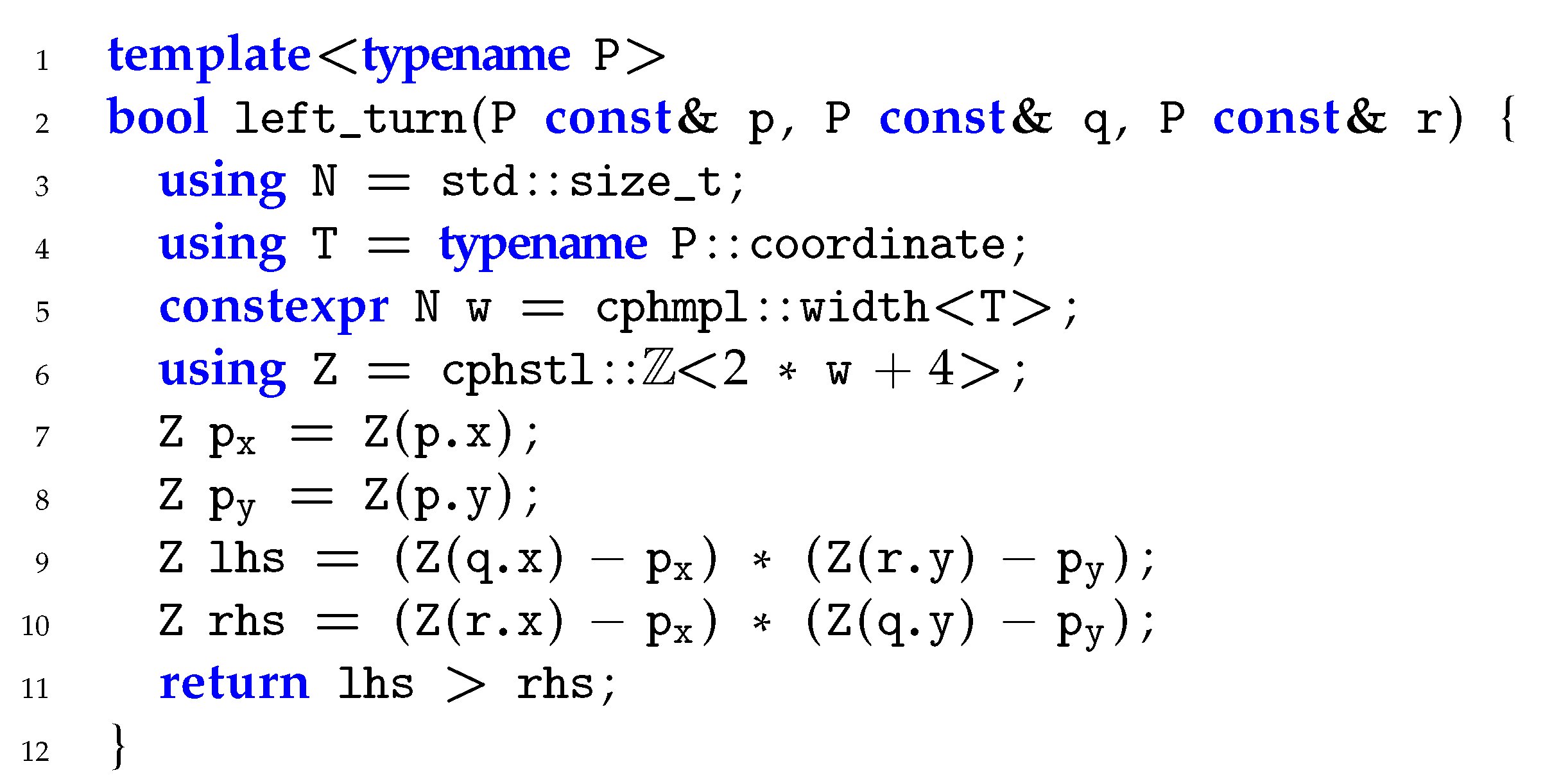
A sequence of points is monotone if the points are sorted according to their x-coordinates—in non-decreasing or non-increasing order. Let p, q, and r be three consecutive vertices on a monotone polygonal chain. Recall that a vertex q of such a chain is concave if there is a left turn or no turn (in the code the condition is not right_turn(p, q, r)) when moving from p to r via q. That is, the angle $\angle pqr$ on the right-hand side with respect to the traversal order is greater than or equal to $\pi$.

The plane-sweep algorithm, proposed by Andrew [3], computes the convex hull for a sequence of points as follows:

(A)

Sort the input points in non-decreasing order according to their x-coordinates.

(B)

Determine the leftmost point (west pole) and the rightmost point (east pole). If there are several pole candidates with the same x-coordinate, let the bottommost of them be the west pole; and on the other end, let the topmost one be the east pole.

(C)

Partition the sorted sequence into two parts, the first containing those points that are above or on the line segment determined by the west pole and the east pole, and the second containing the points below that line segment.

(D)

Scan the two monotone chains separately by eliminating all concave points that are not on the convex hull. For an early description of this backtracking procedure relying on cross-product computations, see [33].

(E)

Concatenate the computed convex chains to form the final answer.

It is worth mentioning that the backtracking procedure used in Step (D) does not work for all polygons as claimed in [33] (for a bug report, see [9]). What is important for our purposes is that it works for monotone polygonal chains provided that the poles are handled as discussed by Andrew [3]: All other points that have the same x-coordinate as the west pole (east pole) are eliminated, except the topmost (bottommost) one provided that it is not a duplicate of the pole. Furthermore, Andrew [3] pointed out that in Step (C) it is only necessary to perform the orientation test for points whose y-coordinate is between the y-coordinates of the west and east poles. Usually, this will reduce the number of orientation tests performed by a significant fraction.

There is a catch hidden in the original description of the algorithm [3]. In Step (C), the partitioning procedure must retain the sorted order of the points, i.e., it must be stable. In Andrew’s description, it is not specified how this step is to be implemented. It is possible to do stable partitioning in place in linear time (see [34]), but all linear-time algorithms developed for this purpose are considered to be galactic. That means they are known to have a wonderful asymptotic behaviour, but they are never used to actually compute anything [35]. Therefore, it is understandable that Gomes’ implementation of torch [4] used extra arrays of indices to carry out multi-way grouping stably.

It is known that the plane-sweep algorithm can be implemented in place. Unfortunately, the description given in [15] does not lead to an efficient implementation; the goal of that article was to show that an in-place implementation is possible.

The problem with stable partitioning can be avoided by performing the computations in a different order: find the west and east poles before sorting. This way, when creating the two candidate collections, we can use unstable in-place partitioning employed in quicksort—for example, the variant proposed by Lomuto ([26], Section 7.1)—and sort the candidate collections separately after partitioning.

Let p and r be two points that are known to be on the convex hull. In our implementation of plane-sweep the key subroutine is chain: It takes an oriented line segment $\overrightarrow{pr}$ and a candidate collection C of points, which all lie on the left of $\overrightarrow{pr}$, and computes the convex chain, i.e., part of the convex hull, from p to r via the points in C. The extreme points are specified by two iterators and the candidate collection is assumed to follow immediately after p in the input sequence. The past-the-end position of the candidate collection is yet another parameter. To make the function generic, so that it can compute both the upper hull and the lower hull, it has a comparator as its last parameter. This comparator specifies the sorting order of the points. As is customary in the C++ standard library, a less-than comparison function orders the points in non-decreasing order and a greater-than comparison function orders them in non-increasing order.

To accomplish its task, chain works as follows: (a) If C is empty, return the position of the successor of p as the answer, i.e., the computed chain consists of p. (b) Sort the candidates in the given order according to their x-coordinates. As a result, the points with equal x-coordinates can be arranged in any order. (c) If in C there are points with the same x-coordinate as p, eliminate all the other except the one having the largest y-coordinate—with respect to the given ordering—before any further processing. (d) Use the standard backtracking procedure [33] to eliminate all concave points from the remaining candidates. The stack is maintained in place at the beginning of the zone occupied initially by p and C coming just after p. This elimination process is semi-stable, meaning that it retains the sorted order of the points in the left part of partitioning; it may change the order of the eliminated points. (e) Return the position of the first eliminated point as the answer (or the past-the-end position of C if all points are convex).

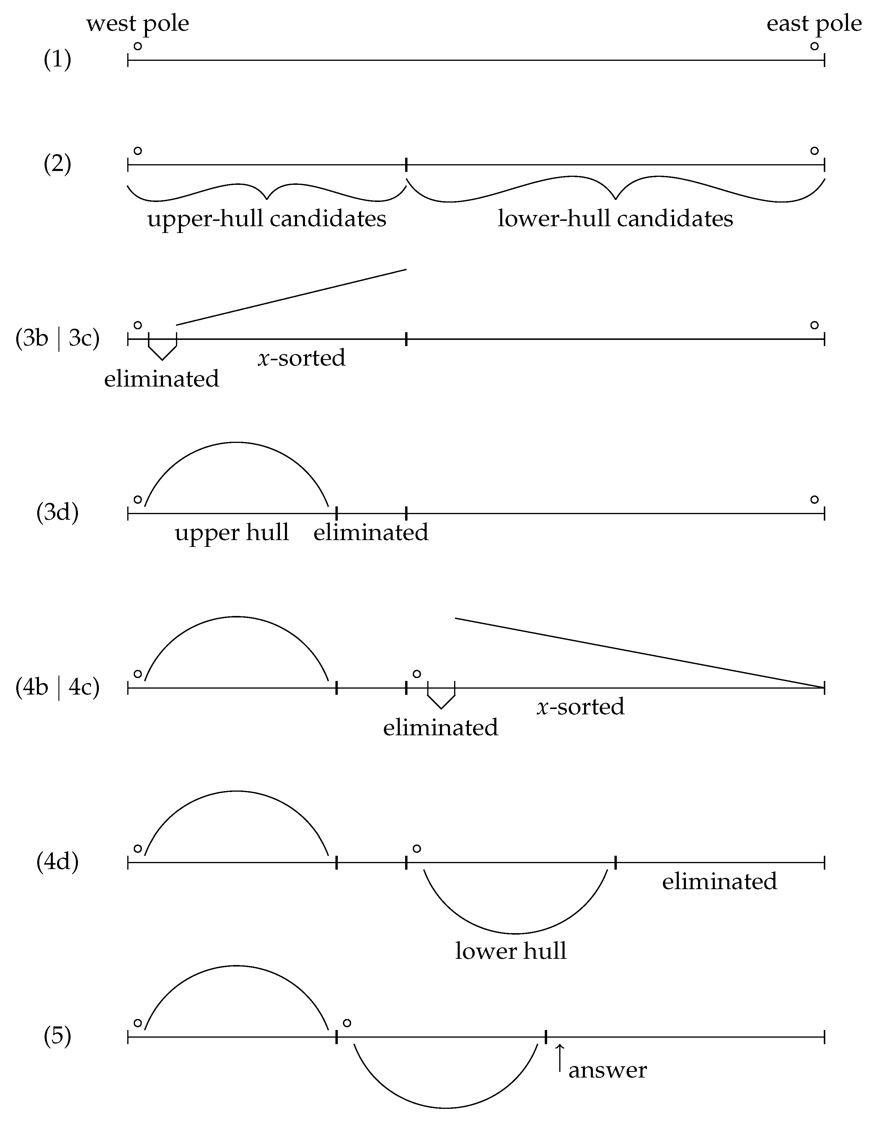
Thus, our in-place implementation of plane-sweep processes any non-empty sequence of points as follows (for an illustration, see Figure 2):

(1)

Find the west and east poles by scanning the input sequence once. Place the poles at their respective ends of the input sequence. If the poles are the same point, stop and return the position of the successor of the west pole.

(2)

Partition the input sequence into two parts: (a) the upper-hull candidates, i.e., the points that are above or on the line segment determined by the west pole and the east pole; and (b) the lower-hull candidates, i.e., the points below that line segment.

(3)

Apply the function chain with the poles, the upper-hull candidates, and comparison function less than. This gives us the upper hull from the west pole to the east pole, excluding the east pole.

(4)

Swap the east pole to the beginning of the lower-hull candidates, and apply the function chain with the two poles—this time giving the east pole first, the lower-hull candidates, and the comparison function greater than. After this we also have the lower hull, but it is not in its final place.

(5)

Move the computed lower hull just after the computed upper hull (if it is not there already). This is a standard in-place block-swap computation. Finally, return the position of the first eliminated point (or the past-the-end position if all points are in the convex hull).

If heapsort [36] was used in the implementation of chain, the whole algorithm would operate in place and run in $O\left(n\lg n\right)$ worst-case time. However, the C++ standard-library introsort [27], which is a combination of quicksort, insertionsort, and heapsort, is known to be more efficient in practice. Still, it guarantees the $O\left(n\lg n\right)$ worst-case running time and, because of careful programming, it operates in situ since the recursion stack is never allowed to become deeper than $2\lg n$.

4.2. Torch

The following definitions are from [37]: (1) A rectilinear line segment is a line segment oriented parallel to either the x-axis or the y-axis. (2) A point set is rectilinear convex if for any two of its points which determine a rectilinear line segment, the line segment lies entirely in the given set. (3) Given a multiset S of points, its (connected) rectilinear convex hull is the smallest connected rectilinear convex set enclosing all the points of S. Roughly speaking, a rectilinear convex hull connects all the maximal points with four rectilinear curves.

At the abstract level, torch [2] operates in two stages: (1) Find the points on the rectilinear convex hull. (2) Refine this approximation by discarding all concave points from it. The correctness of this approach follows directly from the fact that the rectilinear convexity is a looser condition than the normal convexity. Ottmann et al. [37] showed how to compute the rectilinear convex hull in $O\left(n\lg n\right)$ time and $O\left(n\right)$ space. If plane-sweep is used to do the refinement, the overall running time of this procedure is $O\left(n\lg n\right)$. A similar approach was proposed by Bentley et al. [14] (see also [38,39])—they computed all maximal points; they were not interested in the rectilinear curvature. They proved that, under the assumption that the points are chosen from a probability distribution in which each coordinate of a point is chosen independently of all other coordinates, the number of maximal points is $O\left(\lg n\right)$. Using this fact, one can develop algorithms for computing maxima and convex hulls (for a historical review, see [39]), for which the expected running time is $O\left(n\right)$ and the worst-case running time $O\left(n\lg n\right)$.

Gomes [2] combined the rectilinear-convex-hull algorithm by Ottmann et al. [37] and the plane-sweep algorithm [3] as follows: (1) By integrating the two algorithms better, redundant sorting computations can be avoided. (2) By replacing lexicographic sorting with x-sorting, a superset can be computed faster even though now it may include some extra maximal points that lie on the periphery of the rectilinear convex hull—i.e., the computation of the rectilinear convex hull is not fully accurate, but for our purpose these extra maximal points are by no means harmful. We call the points selected by Gomes’ heuristic algorithm boundary points. In torch, Steps (C) and (D) of the plane-sweep algorithm are replaced with the following three steps (for an illustration, see Figure 3):

(B’)

Find the topmost point (north pole) and the bottommost point (south pole) by one additional scan and resolve the ties in a similar fashion as in Step (B).

(C’)

Group the input points into four (overlapping) candidate collections such that, for $i\in \left\{1,2,3,4\right\}$, the i’th collection contains the points that are not dominated by the adjacent poles in the respective direction (north-west, north-east, south-east, or south-west), i.e., these points are in the quadrant $Q_i$ of Figure 3. Note that the quadrant includes the borders.

(D’)

In each of the candidate collections, compute the boundary points before discarding the concave points that are not in the output polygon.

Let us look at Step (D’) a little more thoroughly by considering what is done in $Q_1$: (1) The points in $Q_1$ are sorted according to their x-coordinates. (2) The sorted sequence is scanned from the west pole to the north pole and a point is selected as a boundary point if its y-coordinate is larger than or equal to the maximum y-coordinate seen so far. That is, the selected points form a monotonic sequence both with respect to their x-coordinates and y-coordinates; we call such a sequence a staircase. Since the points on the computed staircase are all maximal and only maximal points on a rectilinear line segment determined by two other points may be discarded, the staircase must contain all vertices of the convex hull that are in $Q_1$. (3) As the final step, the standard backtracking procedure is applied for the points in the staircase to get the part of the convex hull that is inside $Q_1$.

One should observe that the classification, whether a point is a boundary point or not, depends on the original order of the points. For example, consider a multiset of three points $(1,1)$, $(1,2)$, $(1,1)$ given in this order. All these points are dominant in the north-west direction, but the scan only selects the first two as the boundary points. If the order of the last two points had been the opposite, then all three would be classified as boundary points. Since it is unspecified, how a sorting algorithm will order points whose x-coordinates are equal, in our worst-case constructions we assume that such points are ordered so that all maximal points will be classified as boundary points.

The processing in the other quadrants is symmetric. In $Q_2$ the points are scanned from the east pole to the north pole and the staircase goes upwards as in $Q_1$. In $Q_3$ the processing is from the east pole to the south pole and we keep track of the current minimum with respect to the y-coordinates—so the staircase goes downwards. Finally, in $Q_4$ the points are scanned from the west pole to the south pole and the staircase goes downwards as in $Q_3$.

In Step (C’), to do the grouping, it is only necessary to compare the coordinates, the orientation test is not needed. Also, in Step (D’), only coordinate comparisons are done, no arithmetic operations. In the original description [2], the staircases were concatenated to form an approximation of the convex hull before the final elimination scan. However, doing so may cause the algorithm to malfunction—we will get back to the correctness of this approach in Section 5.3.

The asymptotic running time of this algorithm is determined by the sorting steps, which require a total of $\mathrm{\Theta }\left(n\lg n\right)$ time in the worst case and in the average case for the best comparison-based sorting method. If the number of maximal points is small as the theory suggests [14], the cost incurred by the evaluation of the orientation tests will be insignificant. Compared to other alternatives, this algorithm is important for two reasons:

(1)

Only the x-coordinates are compared when sorting the points.

(2)

The number of the orientation tests performed is proportional to the number of maximal points, the coefficient being at most two times the average number of directions the points are dominant in.

As to the use of memory, in the implementation of torch [4], Gomes used

• four arrays of indices—implemented as std::vector—to keep track of the points in each of the four candidate collections,
• an array of points—implemented as std::vector—to store the boundary points in the approximation, and
• a stack—implemented as std::deque—to store the output.

Fact 1.

In the worst-case scenario, Gomes’ implementation may require space for about $8n$ indices and $8n$ points for multiset data (or about $4n$ indices and $4n$ points for set data) for temporary arrays, or $h+512$ points and $\frac{1}{256}h$ pointers for the output stack.

Proof. 

To verify this deficiency for multisets, consider a special input having four poles $(-1,0)$, $(0,1)$, $(1,0)$, $(0,-1)$ and $n-4$ points at the origin. Since the duplicates are on the border, they should be placed in each of the four candidate collections. Hence, each of the index arrays will be of size $n-4$. Since the origin is not dominated by any of the poles, none of the duplicates will be eliminated. Therefore, all the duplicates should be included in the approximation of the convex hull, which may contain about $4n$ points. For sets, in a bad input all input points lie on a line. In this case, all points should be placed in the candidate collections for two of the four quadrants. Again, none of the points on the line are dominated by the poles. Therefore, the approximation may contain $2n$ points.

For C++ standard-library vectors, the total amount of space allocated can be two times larger than what is actually needed (see, for example, the benchmarks reported in [40]). In the C++ standard library, by default a stack is implemented as a deque which is realized by maintaining a vector of pointers to memory segments (of, say, 512 points). From this discussion, the stated bounds follow.  □

It should be emphasized that this heuristic algorithm only reduces the number of orientation tests performed in the average case. There is no asymptotic improvement in the overall running time—in the worst case or in the average case—because the pruning is done after the sorting. The plane-sweep algorithm may perform the orientation test up to about $3n$ times. For the special input described above, torch may perform the orientation test at least $4n-O\left(1\right)$ times, so in the worst case there is no improvement in this respect either. As we utilize an implementation improvement, where not all maximal points are computed, but only those that form a staircase in each of the four quadrants, some of the maximal points may be eliminated already during this staircase formation. Experimentally, the highest number of orientation tests observed to be performed by torch was $3.33n$.

Due to the correctness issues and excessive use of memory, we decided to implement our own version of torch. Our corrected version requires $O\left(1\right)$ or $O\left(\lg n\right)$ words of additional memory, depending on whether heapsort [36] or introsort [27] is used in sorting. After finding the poles, the algorithm processes the points in four phases:

(1a)

Partition the input sequence such that the points in the north-west quadrant ($Q_1$ in Figure 3) determined by the west and north poles are moved to the beginning and the remaining points to the end (normal two-way partitioning).

(1b)

Sort the points in $Q_1$ according to their x-coordinates in non-decreasing order.

(1c)

Find the boundary points in $Q_1$ and move the eliminated points at the end of the zone occupied by the points of $Q_1$. Here the staircase goes upwards.

(1d)

Scan the boundary points in $Q_1$ to determine the convex chain from the west pole to the north pole. Again, the eliminated points are put at the end of the corresponding zone.

(2a)

Consider all the remaining points (also those eliminated earlier) and partition the zone occupied by them into two so that the points in $Q_2$ become just after the west-north chain ending with the north pole.

(2b)

Sort the points in $Q_2$ according to their x-coordinates in non-increasing order.

(2c)

Find the boundary points in $Q_2$ as in Step (1c). Also here the staircase goes upwards.

(2d)

Reverse the boundary points in place so that their x-order becomes non-decreasing.

(2e)

Continue the scan that removes the concave points from the boundary points to get the convex chain from the north pole to the east pole.

(3)

Compute the south-east chain of the convex hull for the points in $Q_3$ as in Step (2), except that now the staircase goes downwards and the reversal of the boundary points is not necessary.

(4)

Compute the south-west chain of the convex hull for the points in $Q_4$ as in Step (2), except that now the sorting order is non-decreasing and the staircase goes downwards.

It is important to observe that any point in the middle of Figure 3 is dominated by one of the poles in each of the four directions. Hence, these points are never moved to a candidate collection. However, if a point lies in two (or more) quadrants, it will take part in several sorting computations. (In Figure 3, move the east pole up and see what happens.) To recover from this, it might be advantageous to use an adaptive sorting algorithm.

4.3. Quickhull

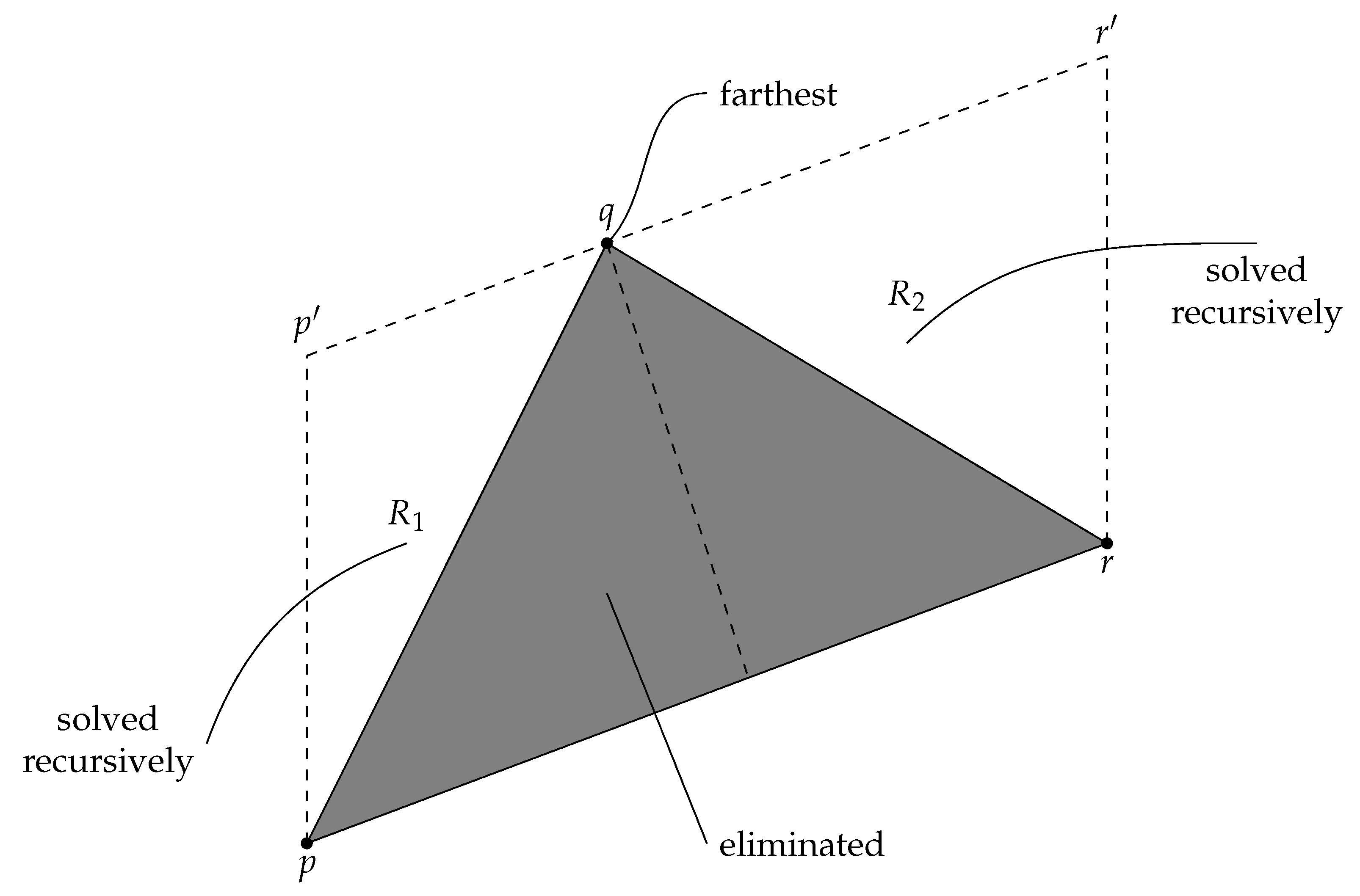
The quickhull algorithm, which mimics quicksort, has been reinvented several times (see, e.g., [8,9,10]). The key subroutine is again the one that chains two extreme points together, but now it is implemented recursively (for a visualization, see Figure 4). The parameters are an oriented line segment $\overrightarrow{pr}$ determined by two extreme points p and r, and a collection C of points on the left side of $\overrightarrow{pr}$. If the cardinality of C is small, we can use any brute-force method to compute the convex chain from p to r, return that chain, and stop. Otherwise, of the points in C, we find an extreme point q in the direction orthogonal to $\overline{pr}$; in the case of ties, we select the leftmost extreme point. Then, we eliminate all the points inside or on the perimeter of the triangle $(p,q,r)$ from further consideration by moving them away to the end of the zone occupied by C. Finally, we invoke the recursive subroutine once for the points of C that are on the left of $\overrightarrow{pq}$, and once for the points of C that are on the left of $\overrightarrow{qr}$. An important feature of this algorithm is that the interior points are eliminated during sorting—full sorting may not be necessary. Therefore, we expect this algorithm to be fast.

Gomes used the qhull program [41] in his experiments. However, he did not give any details how he used this library routine so, unfortunately, we have not been able to repeat his experiments. From the qhull manual [42], one can read that the program is designed to

• solve many geometric problems,
• work in the d-dimensional space for any $d\ge 2$,
• be output sensitive,
• reduce space requirements, and
• handle most of the rounding errors caused by floating-point arithmetic.

Based on this description, we got a feeling that this is like using a sledgehammer to crack a nut. Simply, specialized code designed for finding the two-dimensional convex hull—and only that—should be faster. After doing the implementation work, the resulting code was less than 200 lines long. As an extra bonus,

• we had full control over any further tuning and
• we could be sure that the computed output was correct as, also here, we relied on exact integer arithmetic.

In our implementation of quickhull we followed the guidelines given by Eddy [8] (the space-efficient alternative): (1) As in plane-sweep, find the two poles, the west pole p and the east pole r. Put p first and r last in the sequence. (2) Partition the remaining points between p and r into upper-hull and lower-hull candidates: $C_1$ contains those points that lie above or on the line segment $\overline{pr}$ and $C_2$ those that lie below it. (3) Call the recursive elimination routine described above for the upper-hull candidates with the parameters $\overrightarrow{pr}$ and $C_1$. (4) Move r just after the upper chain computed and the eliminated points after the lower-hull candidates. (5) Apply the recursive elimination routine for the lower-hull candidates with the parameters $\overrightarrow{rp}$ and $C_2$. (6) Now the point sequence is rearranged such that (a) p comes first, (b) the computed upper chain follows it, (c) r comes next, (d) then comes the computed lower chain, and (e) all the eliminated points are at the end. Lastly, return the position of the first eliminated point (or the past-the-end position if no such point exists) as the final answer.

As a matter of fact, the analogy with quicksort [16] is not entirely correct since it is a randomized algorithm—a random element is used as the pivot. Albeit, Barber et al. [41] addressed both randomized and the non-randomized versions of quickhull. Eddy [8] made the analogy with quickersort [43], in which the middle element is used as the pivot and the stack size is kept logarithmic. In our opinion, this analogy is not quite correct either. It would be more appropriate to see the algorithm as an incarnation of the middle-of-the-range quicksort where for each subproblem the minimum and maximum values are determined and their mean is used as the pivot. If the elements being sorted are integers drawn from a universe of size U, the worst-case running time of this variant is $O\left(n\lg U\right)$.

Eddy [8] showed that the worst case of quickhull is $O\left(nh\right)$. However, Overmars and van Leeuwen [44] proved that in the average case the algorithm runs in $O\left(n\right)$ expected time. The result holds when the points are chosen uniformly and independently at random from a bounded convex region. Actually, their proof is stronger, because by exploiting the connection to middle-of-the-range quicksort, it can be applied to get the following:

Fact 2.

When the coordinates of the points are integers drawn from a bounded universe of size U, the worst-case running time ofquickhullis $O\left(n\lg U\right)$.

Proof. 

The key observation made by Overmars and van Leeuwen [44] was that, if in the general recursive step the problem under consideration covers an area of size A (the region of interest must be inside the parallelogram $pr{r}^{\prime }{p}^{\prime }$ in Figure 4), then the total area covered by the two subproblems considered at the next level of recursion is bounded from above by $A/2$ (some regions inside $R_1$ and $R_2$ in Figure 4).

When this observation is applied to the bounded-universe case, we know that the area covered by the topmost recursive call is at most $U^2$. That is, the depth of the recursion must be bounded by $2\lg U$. In the recursion tree, since the subproblems are disjoint, the total work done at each level is at most $O\left(n\right)$. Thus, the running time must be bounded by $O\left(n\lg U\right)$.  □

So, in the bounded-universe case, middle-of-the-range quicksort and quickhull cannot work tremendously badly. As an immediate consequence, if these algorithms are implemented recursively, the size of the recursion stack will be bounded by $O\left(\lg U\right)$.

4.4. Other Elimination Heuristics

The quickhull algorithm brings forth the important issue of eliminating interior points—if there are any—before sorting. When computing the convex hull, one has to consider all directions when finding the extreme points. A rough approximation of the convex hull is obtained by considering only a few specific directions. As discussed in several papers (see, for example, [3,11,12]), by eliminating the points falling inside or on the boundary of such an approximation, the problem size can often be reduced considerably. After this kind of preprocessing, any of the algorithms mentioned earlier could be used to process the remaining points.

For a good elimination strategy two things are important: (1) speed and (2) effectiveness. To achieve high speed, the elimination procedure should be simple. With good elimination effectiveness, the cost of the main algorithm may become insignificant. So there is a trade-off between the two.

Akl and Toussaint [11] found the extrema in four equispaced directions—those determined by the coordinate axes. Also, Andrew [3] mentioned this as an option to achieve further saving in the average-case performance of the plane-sweep algorithm. This poles-first algorithm, as we name it, works as follows: (1) Compute the west, north, east, and south poles. (2) Eliminate the points inside or on the perimeter of the quadrilateral (or triangle or line segment) having these poles as its vertices. (3) Apply the plane-sweep algorithm for the remaining points. The elimination overhead is two scans—so the elimination procedure is fast. Unfortunately, it is not always efficient. For example, in the case that the west and south poles coincide, and the north and east poles coincide, only the points on the line segment determined by the two poles will be eliminated.

Devroye and Toussaint [12] used eight equispaced directions. We name this algorithm throw-away; we implemented it as follows: (1) Find the extreme points in eight predetermined directions: $\pm x$, $\pm y$, $\pm (x+y)$, and $\pm (x-y)$. (2) Eliminate all the points inside or on the boundary of the convex polygon determined by the found points. (3) Apply the plane-sweep algorithm for the remaining points. Also here, the elimination overhead is two scans: one max-finding scan to find the extrema and another partitioning scan to do the elimination. If the plane-sweep algorithm used heapsort, the whole algorithm would work in place; with introsort it works in situ instead.

Devroye and Toussaint [12] proved that for the square data set the number of points left after throw-away preprocessing will be small. Unfortunately, as also pointed out by them, the result depends heavily on the shape of the region, from where the points are drawn randomly.

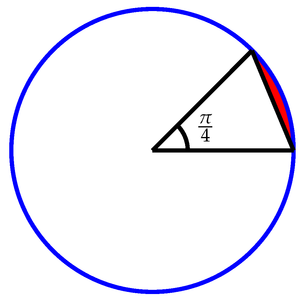
Fact 3.

For the disc data set of size n, the expected number of points left afterthrow-awaypreprocessing is bounded from below by $(1-\frac{2\sqrt{2}}{\pi })n$.

Proof. 

Let r be the radius of the circle, in which the points lie. The preprocessing step finds (up to) eight points. Assume that the polygon determined by the found points covers the largest possible area inside the circle. Trivially, the shape that maximizes the covered area is an equal-sided octagon touching the circle at each of the vertices. Let us now consider one of the sectors defined by two consecutive vertices of such an octagon (see Figure 5). The inside angle of this sector is $\frac{\pi }{4}$. Hence, the area of the sector is $\frac{\pi }{8}{r}^2$. The area of the triangle inside this sector is $\frac{1}{2}{r}^2\sin \left(\frac{\pi }{4}\right)$. Since $\sin \left(\frac{\pi }{4}\right)=\frac{\sqrt{2}}{2}$, the area of the top of the sector inside the circle that is not covered (the red area in Figure 5) is $\frac{\pi r^2}{8}-\frac{\sqrt{2}{r}^2}{4}$. Summing this over all eight sectors, the fraction of the circle that is not covered is $1-\frac{2\sqrt{2}}{\pi }$. This is about $9.968$ %. From this it follows that the expected number of points left after elimination must be larger than $(1-\frac{2\sqrt{2}}{\pi })n$, as claimed.  □

An implementation of the throw-away algorithm was described in [18]. The authors tried to make the integration between the preprocessing step and the plane-sweep algorithm smooth to prevent repetitive work in the latter (recomputation of the poles and orientation tests in partitioning). However, the linear space needed for this integration was a high price to pay because, after elimination, the main bulk of the work is done in sorting.

Yet another alternative is to see quickhull as an elimination algorithm. To integrate quickhull with plane-sweep, we reimplemented it in an introspective way. When the recursion depth reached some predetermined threshold, we stopped the recursion and solved the subproblem at hand using plane-sweep. For integer k, let k-introhull be the member of the family of quickhull algorithms for which the threshold is k. For example, 3-introhull is quite similar to throw-away elimination. The member $\left(\lg n\right)$-introhull is significant, because the amount of work done at the top portion of the recursion tree will be bounded by $O\left(n\lg n\right)$ and the amount of the work done when solving the subproblems at the leaves will also sum up to $O\left(n\lg n\right)$. For this variant, the worst-case running time is $O\left(n\lg n\right)$ as for the plane-sweep algorithm. Still, the average-case running time is $O\left(n\right)$ since the expected number of points left decreases geometrically with recursion depth. From this it follows that the expected number of points left at recursion level $\lg n$ is $O\left(1\right)$.

By the observation of Overmars and van Leeuwen [44], for k-introhull, the expected number of points left after the elimination should at most be around $\frac{1}{2^k}n$ for both of our data sets. To verify this bound in practice, we measured the expected number of points left after elimination for the two data sets. To understand how k-introhull works compared to the other elimination heuristics, we made the same experiments for them, too.

The numbers in

Table 3. The average number of points left after the elimination [%] for different strategies for the two data sets.

n	3-introhull		4-introhull		poles-first		throw-away
	Square	Disc	Square	Disc	Square	Disc	Square	Disc
$2^{10}$	3.37	12.0	0.06	0.30	51.0	37.9	4.29	12.2
$2^{15}$	0.60	10.2	0.02	0.85	50.9	36.5	0.71	10.2
$2^{20}$	0.10	9.99	0.00	0.66	51.3	36.3	0.12	9.99
$2^{25}$	0.01	9.97	0.00	0.64	50.6	36.3	0.01	9.97
$2^{30}$	0.00	9.97	0.00	0.64	50.4	36.3	0.00	9.97

are the averages of many repetitions, except those on the last row. The elimination effectiveness of poles-first is not impressive—although there are no surprises in the numbers. The throw-away algorithm works better; it is designed for the square data set, but the limit $9.968\%$ in the elimination effectiveness for the disc data set leaves some shadows for this algorithm. The numbers for 3-introhull are basically the same as those for throw-away. Roughly speaking, in quickhull all the work is done at a few first recursion levels. Compared to the static throw-away algorithm, the elimination strategy applied in quickhull is adaptive, and it can be made finer by increasing k. If good worst-case efficiency is important and one wants to use quickhull, we can warmly recommend $\left(\lg n\right)$-introhull. The overhead compared to the standard set-up is one if statement in each recursive call to check if the leaf level has been reached. So the worst-case performance of quickhull can be reduced from $O\left(n\lg U\right)$ to $O\left(n\lg n\right)$ if wanted.

5. Testing

When writing the programs for this paper, we tried to follow good industrial practices. First, we made frequent reviews of each other’s code. Second, we built a test suite that could be used to check the answers computed. Only after the programs passed the tests did we benchmark them. One more time we experienced that programming is difficult. Even if the test suite had only a dozen, or so, test cases, it took time before each of the programs passed the tests. Furthermore, the test suite was useful in regression testing when we tuned our programs.

5.1. Test Framework

To be able to verify the correctness of the output automatically, three functions were implemented: same_multiset, convex_polygon, and all_inside. The first function same_multiset takes two multisets of n and m points (both specified by a pair of iterators) as its arguments and checks whether these multisets are the same. If $n\ne m$, this task is trivial. Otherwise, we copied the given multisets, sorted the copies lexicographically, and verified that the sorted sequences were equal. The second function convex_polygon takes a multiset of h points (specified by a pair of iterators) as its argument and checks whether the given points form the consecutive vertices of a convex polygon. The third function all_inside takes a multiset of n points and a convex polygon of h vertices (both specified by a pair of iterators) as its arguments and checks whether all the points in the multiset are inside or on the boundary of the convex polygon.

The function same_multiset is easily seen to require $O\left(n\lg n\right)$ time in the worst case. To implement the function convex_polygon in $O\left(h\right)$ worst-case time, we took inspiration from ([26], Exercise 33.1-5). The function all_inside runs in $O\left(n\lg h\right)$ worst-case time since it performs two binary searches over the convex polygon of size h for each of the n points.

The test suite has—among others—the following test cases, each implemented as a separate function. The names of the test cases were selected to indicate what is being tested:

• empty_set,
• one_point,
• two_points,
• three_points_on_a_vertical_line,
• three_points_on_a_horizontal_line,
• ten_equal_points,
• four_poles_with_duplicates,
• random_points_on_a_parabola,
• random_points_in_a_square (10,000 test cases),
• corners_of_the_universe.

As one can see from this list, we expect that the programs are able to handle multiset data, degenerate cases, and arithmetic overflows.

To use the test suite, every algorithm must be implemented in its own namespace which provides a function solve to be used to compute convex hulls and a function check to be used to check the validity of the answer. Normally, a checker takes a copy of the input, solves the problem with a solver, and uses the tools in our test suite to check that the points in the output are the same as those in the input, that the computed hull is a convex polygon, and that all the input points are inside or on the boundary of the computed convex hull. That is, the programs can be made self-testing if wanted—but the time and space overhead for doing this is quite high due to sorting and extra copies taken.

5.2. Test-First Development

For each of our programs serious debugging has been necessary. At the very beginning, the test framework was primitive; it checked the answers in quadratic time. Thereafter, a natural workflow was to repeatedly write a new implementation and test it. The implementation under consideration was corrected whenever necessary. The test framework was gradually improved when we understood the corner cases better. As shown in Section 5.3, we succeeded in using the test framework to reveal an error at the algorithm level. However, its main purpose was to help remove some small embarrassing errors from the code.

To simplify the implementation task, we used the generic functions of the C++ standard library whenever possible, e.g., std::sort, std::minmax_element, std::max_element, std::partitioning, std::reverse. The consequence of this choice was that our code relies on iterators, array indexing is not used.

When looking at our code, sometimes there seem to be unnecessary complications. Often, however, these complications are there to fix some correctness issue. The basic reason for a complication—which can just be an irritating if statement—is the expectation that the programs must be able to handle multiset data, degenerate cases, and arithmetic overflows. To understand such complications better and to make it easier for others to develop reliable code, we list below some problem areas where we made programming errors. It is imperative to emphasize that the test framework was the most important aid to detect these issues.

• Small instances. It is trivial to handle the cases $n=0$ and $n=1$, but already the case $n=2$ introduces a complication: If the two points are duplicates, special handling is necessary. For larger n, it is also possible that the west pole and the east pole coincide, so this special case must be handled separately.
• Referential integrity. Let p and q be two iterators pointing to some elements. A typical way of swapping these elements is to invoke std::iter_swap(p, q). An unfortunate consequence of this swap is that the iterators are not valid after this operation. It may be necessary to execute std::swap(p, q) just after it. The situation becomes worse when there is another iterator r pointing to the same position as p or q. After the swap, this iterator is not valid any more.
• Empty ranges. Often a subroutine expects to get a range specifying a sequence of elements. In most cases the range is non-empty, but we should also be prepared to handle the empty case.
• Duplicates. These can appear in many places, including places where you do not expect them. For a set of points in general position, it may be enough to execute a single assignment, but in the case of duplicates we may need a loop to jump over them.
• Points on a rectilinear line. When several points are on the same rectilinear line and this happens when finding a pole, a rule is needed to know which one to choose. To break the tie, we use lexicographic ordering even though we want to avoid it in sorting. In a typical case, there is only one pole per direction, so we wanted to avoid the overhead of maintaining two poles per direction, i.e., the bottommost west pole and the topmost west pole.
• Elimination of concave points. After a pole is found, there may be other points on the same rectilinear line. The standard backtracking procedure [33] is not always able to process collinear points correctly. Therefore, a separate routine is needed to find the next convex-hull point that is on the same line and farthest away from the found pole.
• Points on a line. When finding the farthest point from a line segment and several points are equally far, it is necessary to use lexicographic ordering as a tiebreaker. Again, the reason is the standard backtracking procedure—it may fail if collinear points are not processed in the correct order.
• Index arithmetic. When computing the convex hull in pieces, the points may not be in consecutive positions any more. For example, it may be necessary to perform index arithmetic modulo n to get access to the west pole when processing the lower hull after the upper hull has already be computed. Because we operate on iterators, this index arithmetic is not allowed. Therefore, it may be necessary to add some additional parameters for the functions or it may even be convenient to have two copies of the same function where the other takes care of some special case.

Often it is not difficult to handle these special cases correctly, but it may be difficult for a programmer to spot where the fixes are necessary. Luckily, after correcting the code, the performance is not degenerated. It is only a question to produce the correct output.

5.3. Uncovering Algorithm Vulnerability

When using our test framework to test Gomes’ code [4], we realized that not only the program, but the underlying algorithm was incorrect. In the following narration, we will verify this claim.

Let us recall the operating principle of Gomes’ version of torch [2]. There are four basic steps: (1) Find the poles by scanning the input sequence twice. (2) Compute the boundary points in each of the four quadrants. This gives us up to four staircases. (3) Concatenate the staircases to form an approximation of the convex hull. (4) Remove all concave points from this approximation using the standard backtracking procedure [33]. Be aware that the algorithm tries to compute the vertices of the convex hull in counterclockwise order.

The backtracking procedure is known to work for a star-shaped polygon, but one has to be careful if there are duplicates or if there are several points with the same polar angle when sorted around the centre of the polygon—as explained in [5]. It also works for a monotone polygonal chain, provided that the poles are treated separately—as explained in [3]. But the procedure may fail for a self-intersecting polygon—as reported in [9].

Fact 4.

The backtracking procedure—as it is used by the original version oftorchto eliminate all concave vertices from a simple polygon—may fail if some of the vertices overlap.

Proof. 

As a concrete example, consider an input sequence that contains four points from the parabola $y=x^2$: $(3,9)$, $(1,1)$, $(2,4)$, $(0,0)$. All these points are maximal and, since they are monotone in the y-direction, none of them will be eliminated during the staircase formation. There are two staircases: one going up from the origin via the other points to the top and another going down the same way from the top to the origin. Thus, the approximation contains seven points: $(0,0)$, $(1,1)$, $(2,4)$, $(3,9)$, $(2,4)$, $(1,1)$, $(0,0)$. When this polygon is processed using the standard backtracking procedure, the (incorrect) output has two points: $(0,0)$ and $(1,1)$.

The problem is that the orientation predicate cannot distinguish the cases whether the turning angle, when traversing from a point to another point via a third point, is equal to $\pi$ or $2\pi$. Hence, when the test is applied to the points $(2,4)$, $(3,9)$, and $(2,4)$, the middle point will be eliminated—which is a wrong decision. The problem also occurs when there are several points on a vertical line. If the points with the same x-coordinate are not sorted according to their y-coordinates, it can happen that the topmost point will be wrongly eliminated.  □

Since we process the staircases one by one, they are monotone in the x-direction, and we handle the poles separately (collinear points are only a problem at the poles), the correctness of our approach follows directly from the work of Andrew [3].

6. Workhorse Experiments

Now we are ready to investigate the state of algorithms that solve the convex-hull problem in the plane. We selected the following four competitors for further experiments: plane-sweep (Section 4.1), torch (Section 4.2), quickhull (Section 4.3), and throw-away (Section 4.4). As a point of reference, we also made measurements for the standard-library sort function, referred as introsort [27], which was used to sort the points according to their x-coordinates. The theoretical performance of these algorithms is summarized in

Table 4. A summary of the theoretical performance of the algorithms considered. The average-case running time is for the square data set. Here n denotes the size of the input, U the size of the coordinate universe, and $W\left(n\right)$ the amount of the work space required by the sorting routine in use. [*] means that the result was presented in this paper.

Algorithm	Worst Case	Average Case	Work Space
introsort [27]	$\mathrm{\Theta }\left(n\lg n\right)$	$\mathrm{\Theta }\left(n\lg n\right)$	$W\left(n\right)\equiv O\left(\lg n\right)$
plane-sweep [3]	$\mathrm{\Theta }\left(n\lg n\right)$	$\mathrm{\Theta }\left(n\lg n\right)$	$O\left(1\right)+W\left(n\right)$ [15] [*]
torch [2]	$\mathrm{\Theta }\left(n\lg n\right)$	$\mathrm{\Theta }\left(n\lg n\right)$	$O\left(1\right)+W\left(n\right)$ [*]
quickhull [8,9,10]	$O\left(n\lg U\right)$ [*]	$\mathrm{\Theta }\left(n\right)$ [44]	$O\left(\lg U\right)$ [*]
throw-away [12]	$\mathrm{\Theta }\left(n\lg n\right)$	$\mathrm{\Theta }\left(n\right)$	$O\left(1\right)+W\left(n\right)$ [*]

. The goal of the experiments was to see if the theory is able to capture the practical behaviour correctly.

6.1. Experimental Design

To make the programs robust, we considered three alternative approaches when implementing the geometric primitives:

• Multi-precision arithmetic. As described in Section 2.3, we performed intermediate calculations using the multi-precision integers available at the CPH STL [22]. This solution is generic, works for any type of integer coordinates, and the program code is beautiful.
• Double-precision arithmetic. We specialized the geometric primitives to use double-precision integers (signed/unsigned long long), kept track of all the possible overflows, and dealt with them accordingly. This ad-hoc solution relies on the fact that the coordinates are of type int. Unfortunately, we must admit that the resulting code is inelegant.
• Floating-point filter. We converted the coordinates to floating-point numbers and performed the intermediate calculations using them. Only if the result was not known to be correct due to accumulation of rounding errors would we use the multi-precision numbers to redo the calculations. In the present case, we employed Shewchuk’s filter coded in [45]. A readable explanation of how the filter works can be found in [46].

Most of our programs can be run in any of the three modes just by specifying which arithmetic to use in the realization of the geometric primitives.

In our experiments, we fixed the coordinates of the points to be integers of type int, each occupying 32 bits. Hence, the multi-precision solution had to use integers that were wider than any of the built-in integers. The double-precision solution could operate on built-in integers of 64 bits. In our micro-benchmarks, the ad-hoc solution that solely relied on built-in types was the fastest of these three approaches. When the coordinates were of type int, we did not want to slow down the programs unnecessarily, so we used the ad-hoc solution in the experiments reported here. Since we are not reliant on any multi-precision integer library, it should be easier for others to replicate the experiments and reproduce the results.

In earlier studies, the number of orientation tests and that of coordinate comparisons have been targets for optimization. Since the algorithms reorder the points in place, the number of coordinate moves is also a relevant performance indicator. Hence, in addition to the amount of CPU time, we measured the number of orientation tests, coordinate comparisons, and coordinate moves. The number of orientation tests performed is proportional to n in the worst case for plane-sweep, torch, and throw-away; and in the average case for quickhull. The number of coordinate comparisons and coordinate moves is proportional to $n\lg n$ in the worst and average cases for plane-sweep and torch, and to n in the average case for quickhull and throw-away.

6.2. Time Performance

In our first set of experiments, we measured the amount of CPU time used by the competitors to compute the convex hull for the considered data sets. The results are shown in

Table 5. The running time of the competitors [in nanoseconds per point] for the square data set: (a) Linux computer, (b) Windows computer.

(a)
$\mathit{n}$	introsort	plane-sweep	torch	quickhull	throw-away
$2^{10}$	36.65	55.92	49.62	34.67	27.32
$2^{15}$	54.03	72.18	64.68	30.92	26.02
$2^{20}$	71.48	89.24	82.40	31.06	24.40
$2^{25}$	89.37	107.9	101.1	30.78	25.03
$2^{30}$	162.7	281.3	334.4	245.8	247.4
(b)
$\mathit{n}$	introsort	plane-sweep	torch	quickhull	throw-away
$2^{10}$	40.52	53.27	62.40	51.98	34.50
$2^{15}$	64.37	73.86	84.40	48.67	30.90
$2^{20}$	83.76	94.82	106.5	49.54	30.52
$2^{25}$	106.8	124.6	130.4	48.92	30.58

(square),

Table 6. The running time of the competitors [in nanoseconds per point] for the disc data set: (a) Linux computer, (b) Windows computer.

(a)
$\mathit{n}$	introsort	plane-sweep	torch	quickhull	throw-away
$2^{10}$	36.31	52.75	55.01	33.04	27.31
$2^{15}$	53.84	69.10	69.94	30.90	26.96
$2^{20}$	71.20	86.21	87.37	31.06	28.33
$2^{25}$	88.94	104.1	105.4	31.59	30.96
$2^{30}$	212.5	281.3	350.9	226.3	242.3
(b)
$\mathit{n}$	introsort	plane-sweep	torch	quickhull	throw-away
$2^{10}$	40.16	58.66	58.62	47.48	32.84
$2^{15}$	62.19	78.96	79.67	44.64	32.41
$2^{20}$	85.24	101.9	102.2	45.31	34.13
$2^{25}$	108.6	126.6	125.7	46.46	36.29

(disc), and

Table 7. The running time of the competitors [in nanoseconds per point] for the bell data set: (a) Linux computer, (b) Windows computer.

(a)
$\mathit{n}$	introsort	plane-sweep	torch	quickhull	throw-away
$2^{10}$	36.94	53.68	49.96	14.41	20.01
$2^{15}$	54.05	70.67	64.97	12.92	19.12
$2^{20}$	71.11	88.02	81.72	13.22	18.78
$2^{25}$	88.96	105.8	102.5	11.51	18.67
$2^{30}$	224.2	283.0	308.5	152.2	226.3
(b)
$\mathit{n}$	introsort	plane-sweep	torch	quickhull	throw-away
$2^{10}$	40.10	53.51	60.39	22.11	25.95
$2^{15}$	62.68	73.19	82.24	20.32	24.18
$2^{20}$	84.98	95.27	104.6	20.38	23.29
$2^{25}$	114.0	124.9	128.8	20.05	23.55

(bell). The results are unambiguous: For randomly generated data, both quickhull and throw-away are quick! Both of these methods can avoid the sorting bottleneck, which torch does not try to do. We could force quickhull to perform worse than the others when the points were drawn from an arc of a parabola. However, we could only make it a constant factor slower; we could not provoke the $\mathrm{\Theta }\left(nh\right)$ behaviour because of the restricted precision of the coordinates.

When looking at the results, it is eye-catching that, in the Linux computer, the numbers are exceptionally high for the largest problem instance. We observed that, when the size of the input was close to the maximum capacity of main memory, the memory operations became more expensive. The changes in the running times looked normal up to $n=2^{29}$, but after this saturation point the slowdown was noticeable.

In most cases the execution time per point increases as the input instances get larger, while in some cases the cost may stagnate or even get smaller. A logarithmic increase indicates a dominating $O\left(n\lg n\right)$ cost, as the execution times are divided by n. Sorting naturally follows this growth. As both torch and plane-sweep sort a fraction of points a few times, the cost of both is in direct relation to the sorting cost. Both quickhull and throw-away are not directly bounded by this, since they perform some elimination before reverting to sorting. Especially, we note that quickhull tends to become slightly faster (per point) on larger instances. There is a trade-off between the amount of work used for elimination and that used for sorting the remaining points. For randomly generated data, h tends to grow much slower than n, so for quickhull and throw-away the cost incurred by sorting will gradually vanish.

In terms of speed, torch has three success criteria: (1) It should be faster than plane-sweep that it attempts to improve upon; (2) it should perform almost as well as sorting; and (3) it should perform well when compared to other algorithms of industrial standard, as it would otherwise be out-competed by those. For problem instances of low and medium sizes on a square (Table 5) and on a disc (Table 6), torch is placed well in between introsort and plane-sweep. It performs a bit worse in the Windows environment for the bell data set (Table 7), likely because of the earlier-mentioned problem with overlapping work.

We notice that torch becomes relatively slower for large instances. This may be due to the fact that it tries to make the linear term of the cost smaller. To achieve this, it may be necessary to process the same points several times. Thus, for large data collections, its advantage over plane-sweep decreases. There is a trade-off between the elimination cost and the obtained gain. The elimination cost grows with an extra factor of $c\lg n$ per point, albeit with a small constant c, while the saving is a constant per point. As for the third criterion, torch struggles hard with throw-away and quickhull, which are clearly faster, since they eliminate points before sorting, causing the sorting term to grow slower.

One should also notice that the programs behave differently on different computers. On the Linux computer, with some exceptions, torch performs better than plane-sweep, but not significantly better. On the Windows computer, the situation is the opposite between the two. Also, quickhull is slower in the Windows environment. This indicates that the orientation tests can be evaluated faster on the Linux computer, which coincide with indications from our micro-benchmarks. The differences can come from several sources, but we consider it likely that different types of CPUs, compilers, operating systems, and hardware architectures have contributed to this. These differences serve as a warning to those who wish to crown a specific algorithm as the champion, since even with reasonable statistical accuracy, there can be a significant difference in how well a given algorithm performs in different environments.

6.3. Other Performance Indicators

In our second set of experiments, we considered the behaviour of the competitors for the other performance indicators. The average-case scenario was considered, i.e., the coordinates were random ints (square). These experiments were carried out by using a coordinate type that increased a counter each time a comparison, a move, or an orientation test was executed.

The obtained counts are shown in

Table 8. The number of orientation tests executed by the competitors [divided by n] for the square data set.

n	plane-sweep	torch	quickhull	throw-away
$2^{10}$	2.31	0.02	4.95	2.04
$2^{15}$	2.34	0.00	4.86	2.01
$2^{20}$	2.34	0.00	4.82	2.00
$2^{25}$	2.39	0.00	4.70	2.00
$2^{30}$	2.09	0.00	5.37	2.00

(orientation tests),

Table 9. The number of coordinate comparisons performed by the competitors [divided by n] for the square data set.

n	introsort	plane-sweep	torch	quickhull	throw-away
$2^{10}$	12.0	14.8	21.3	2.26	15.0
$2^{15}$	18.1	20.9	28.0	2.25	15.0
$2^{20}$	24.2	27.1	35.3	2.25	15.0
$2^{25}$	30.2	33.3	42.3	2.25	15.1
$2^{30}$	36.5	39.0	49.2	2.25	15.2

(coordinate comparisons), and

Table 10. The number of coordinate moves performed by the competitors [divided by n] for the square data set.

n	introsort	plane-sweep	torch	quickhull	throw-away
$2^{10}$	19.1	30.1	21.3	15.2	21.2
$2^{15}$	26.2	37.2	28.0	14.7	20.2
$2^{20}$	33.3	44.3	35.3	14.5	20.1
$2^{25}$	40.5	51.5	42.3	14.5	20.0
$2^{30}$	47.4	57.8	49.2	16.4	20.4

(coordinate moves). From these numbers it is clear that, for the square data set, both quickhull and throw-away run in linear expected time. As to the orientation tests, torch is a clear winner; since the coordinates are generated independently for the square data set, the expected number of orientation tests executed is $O\left(\lg n\right)$, which explains the zeros. As to the number of coordinate comparisons, torch comes last because interior points take part in four partitioning processes and some of them may also take part in more than one sorting process since the quadrants can overlap. As to the number of coordinate moves, despite repeated work in partitioning, torch performs better than plane-sweep since fewer moves are done in partitioning and in scanning, and the sorting tasks are smaller.

7. Conclusions

We repeat our general conclusion that the quality of implementation really matters in experimental studies. A solid implementation should be based on a correct algorithm. Additional proper testing is necessary before running any experiments. As showcased by this paper, failing to do this may lead to unreliable results and questionable conclusions. The bottom line is that the value of experimental results and their contribution to science are strictly limited by the quality of implementation.

We would like to summarize our findings as follows.

• Robustness. Everyone in computer science knows the problems associated with arithmetic overflows. In the convex-hull algorithms, one has to analyse a single-line formula to determine the maximum precision needed when doing the calculations in an orientation test. This is a type function that maps the type of the input coordinates to the type of some higher-precision numeric type. This mapping can be carried out at compile time. This solution leads to fast performance since the compiler can optimize the generated code. Our message is that a heavyweight static-analysis tool, described in [47], to do automatic code analysis may be an overkill in this particular application, even thought the aim is the same—perform as much work at compile time as possible. On the other end, arbitrary-precision arithmetic provided, for example, by GMP [48] may also be an overkill because the width of the numbers is extended dynamically at run time.
• Correctness. Experimental results can be misleading if the programs do not produce a correct answer. Naturally, testing is not enough to guarantee correctness, but it is a necessary evil to avoid great humiliation. In the case of convex-hull algorithms, a test framework similar to ours can help improve code quality.
• Space requirements. By using less memory, one can avoid the overhead caused by memory management and incur less cache misses. There is a big difference if the amount of extra space used is $\mathrm{\Theta }\left(n\right)$ or $O\left(1\right)$ words. We explained how plane-sweep, torch, poles-first, and throw-away can be implemented in place.
• Arithmetic complexity. For in-situ variants in the integer-arithmetic setting, our experiments indicate that the improvement provided by torch compared to plane-sweep is marginal. However, the situation may change if the arithmetic operations are expensive. Namely, it is expected that torch will execute a fewer number of arithmetic operations than the other investigated algorithms, which always perform $\mathrm{\Omega }\left(n\right)$ orientation tests.
• Reproducibility. In experimental work, a “key principle is that the experiment should be verifiable and reproducible” ([1], Chapter 14). All the programs and scripts used to run the experiments discussed in this paper are publicly available; a frozen release is available as a supplement from the journal (https://www.mdpi.com/1999-4893/11/12/195/s1) and the latest updated release from the home page of the CPH STL [49].

The focus in this paper was on correctness and quality—both in the implementations and experiments. If raw speed is what you need, you may follow some of the following avenues:

• Smarter sorting. In a sorting-based approach, when sorting a sequence of points according to their x-coordinates, if two points are seen to have the same x-coordinate, the point with the smaller (or larger) y-coordinate could be eliminated. More generally, it is possible to sort n elements having at most ℓ different values in $O\left(n\lg \ell \right)$ worst-case time. Another possibility is to use bucketsort when sorting the points [28].
• Further tuning. In this study, quickhull was one of the winners. However, a careful analysis shows that quickhull does redundant orientation tests (as pointed out in [28,50]). By removing some of the redundant work, quickhull can be made even quicker.
• More aggressive elimination. The idea of eliminating interior points during the computation is good! However, in contemporary computers, sorting is fast. So an elimination procedure should not be complicated. In a follow-up paper [51], we implemented a bucketing algorithm ([52], Section 4.4), for which the elimination overhead is three scans and the elimination effectiveness is better than that for the throw-away algorithm. The work space used by this algorithm is $O\left(\sqrt{n}\right)$ words, but because of random access its competitive advantage may fade away when the problem size becomes large.
• Better integration. Many good algorithms are hybrids of several other algorithms. One of the goals is to reach good worst-case and average-case performance at the same time. Taking inspiration from introsort [27], we proposed introhull that combines quickhull [8] and plane-sweep [3]. Gomes’ torch [2] combines the rectilinear-convex-hull algorithm by Ottmann et al. [37] and plane-sweep. However, because of introsort, the average-case running of this hybrid is $\mathrm{\Theta }\left(n\lg n\right)$. As shown by Bentley et al. [14], a divide-and-conquer algorithm could be used to compute a superset which will reduce the average case of the combined algorithm to $O\left(n\right)$, keeping the worst case unchanged. Does this pruning-before-sorting approach have any practical significance?
• Parallel processing. In our benchmarks, only one core was in use even though both of our test computers had four cores. Some previous studies (see, e.g., [53]) have shown that the additional cores can be used to speed up Quicksort, Quickhull, and other divide-and-conquer algorithms. A further study, where speed is at the focus, must consider how technological changes affect the existing algorithms.

References

1. Zobel, J. Writing for Computer Science, 3rd ed.; Springer: London, UK, 2014. [Google Scholar]
2. Gomes, A.J.P. A total order heuristic-based convex hull algorithm for points in the plane. Comput. Aided Des. 2016, 70, 153–160. [Google Scholar] [CrossRef]
3. Andrew, A.M. Another efficient algorithm for convex hulls in two dimensions. Inf. Process. Lett. 1979, 9, 216–219. [Google Scholar] [CrossRef]
4. Gomes, A.J.P. Git Repository. Available online: https://github.com/mosqueteer/TORCH/ (accessed on 2 October 2018).
5. Graham, R.L. An efficient algorithm for determining the convex hull of a finite planar set. Inf. Process. Lett. 1972, 1, 132–133. [Google Scholar] [CrossRef]
6. Jarvis, R.A. On the identification of the convex hull of a finite set of points in the plane. Inf. Process. Lett. 1973, 2, 18–21. [Google Scholar] [CrossRef]
7. Chan, T.M. Optimal output-sensitive convex hull algorithms in two and three dimensions. Discrete Comput. Geom. 1996, 16, 361–368. [Google Scholar] [CrossRef] [Green Version]
8. Eddy, W.F. A new convex hull algorithm for planar sets. ACM Trans. Math. Softw. 1977, 3, 398–403. [Google Scholar] [CrossRef]
9. Bykat, A. Convex hull of a finite set of points in two dimensions. Inf. Process. Lett. 1978, 7, 296–298. [Google Scholar] [CrossRef]
10. Green, P.J.; Silverman, B.W. Constructing the convex hull of a set of points in the plane. Comput. J. 1979, 22, 262–266. [Google Scholar] [CrossRef] [Green Version]
11. Akl, S.G.; Toussaint, G.T. A fast convex hull algorithm. Inf. Process. Lett. 1978, 7, 219–222. [Google Scholar] [CrossRef]
12. Devroye, L.; Toussaint, G.T. A note on linear expected time algorithms for finding convex hulls. Computing 1981, 26, 361–366. [Google Scholar] [CrossRef]
13. McGeorg, C.C. A Guide to Experimental Algorithmics; Cambridge University Press: Cambridge, UK, 2012. [Google Scholar]
14. Bentley, J.L.; Kung, H.T.; Schkolnick, M.; Thompson, C.D. On the average number of maxima in a set of vectors and applications. Inf. Process. Lett. 1978, 25, 536–543. [Google Scholar] [CrossRef]
15. Brönnimann, H.; Iacono, J.; Katajainen, J.; Morin, P.; Morrison, J.; Toussaint, G. Space-efficient planar convex hull algorithms. Theor. Comput. Sci. 2004, 321, 25–40. [Google Scholar] [CrossRef]
16. Hoare, C.A.R. Quicksort. Comput. J. 1962, 5, 10–16. [Google Scholar] [CrossRef] [Green Version]
17. Kettner, L.; Mehlhorn, K.; Pion, S.; Schirra, S.; Yap, C. Classroom examples of robustness problems in geometric computations. Comput. Geom. 2008, 40, 61–78. [Google Scholar] [CrossRef]
18. Bhattacharya, B.K.; Toussaint, G.T. Time- and storage-efficient implementation of an optimal planar convex hull algorithm. Image Vis. Comput. 1983, 1, 140–144. [Google Scholar] [CrossRef]
19. McQueen, M.M.; Toussaint, G.T. On the ultimate convex hull algorithm in practice. Pattern Recognit. Lett. 1985, 3, 29–34. [Google Scholar] [CrossRef]
20. Warren, H.S., Jr. Hacker’s Delight, 2nd ed.; Addison-Wesley Professional: Westford, MA, USA, 2012. [Google Scholar]
21. Katajainen, J. Pure Compile-Time Functions and Classes in the CPH MPL; CPH STL report 2017-2; Department of Computer Science, University of Copenhagen: Copenhagen, Denmark, 2017; Available online: http://hjemmesider.diku.dk/~jyrki/Myris/Kat2017R.html (accessed on 27 November 2018).
22. Katajainen, J. Class templates Z <b> and N <b> for fixed-precision arithmetic. 2018; work in progress. [Google Scholar]
23. Schirra, S. Robustness and precision issues in geometric computation. In Handbook of Computational Geometry; Sack, J.-R., Urrutia, J., Eds.; Elsevier: Amsterdam, The Netherlands, 2000; pp. 597–632. [Google Scholar]
24. Sanders, P. Presenting data from experiments in algorithmics. In Experimental Algorithmics—From Algorithm Design to Robust and Efficient Software; Fleischer, R., Moret, B., Meineche Schmidt, E., Eds.; Springer: Berlin/Heidelberg, Germany, 2002; LNCS; Volume 2547, pp. 181–196. [Google Scholar] [CrossRef]
25. GeeksforGeeks. Convex Hull ∣ Set 2 (Graham Scan). Available online: http://www.cdn.geeksforgeeks.org/convex-hull-set-2-graham-scan/ (accessed on 2 October 2018).
26. Cormen, T.H.; Leiserson, C.E.; Rivest, R.L.; Stein, C. Introduction to Algorithms, 3rd ed.; The MIT Press: Cambridge, MA, USA, 2009. [Google Scholar]
27. Musser, D.R. Introspective sorting and selection algorithms. Softw. Pract. Exp. 1997, 27, 983–993. [Google Scholar] [CrossRef]
28. Allison, D.C.S.; Noga, M.T. Some performance tests of convex hull algorithms. BIT Numer. Math. 1984, 24, 2–13. [Google Scholar] [CrossRef] [Green Version]
29. Bhattacharya, B.K.; Sen, S. On a simple, practical, optimal, output-sensitive randomized planar convex hull algorithm. J. Algorithms 1997, 25, 177–193. [Google Scholar] [CrossRef]
30. Chan, T.M.Y.; Snoeyink, J.; Yap, C.K. Output-sensitive construction of polytopes in four dimensions and clipped Voronoi diagrams in three. In Proceedings of the 6th Annual ACM-SIAM Symposium on Discrete Algorithms, San Francisco, CA, USA, 22–24 January 1995; pp. 282–291. [Google Scholar]
31. Kirkpatrick, D.G.; Seidel, R. The ultimate planar convex hull algorithm? SIAM J. Comput. 1986, 15, 287–299. [Google Scholar] [CrossRef]
32. Wenger, R. Randomized quickhull. Algorithmica 1997, 17, 322–329. [Google Scholar] [CrossRef]
33. Sklansky, J. Measuring concavity on a rectangular mosaic. IEEE Trans. Comput. 1972, C-21, 1355–1364. [Google Scholar] [CrossRef]
34. Katajainen, J.; Pasanen, T. Stable minimum space partitioning in linear time. BIT Numer. Math. 1992, 32, 580–585. [Google Scholar] [CrossRef] [Green Version]
35. Lipton, R.J. Galactic Algorithms. Available online: https://rjlipton.wordpress.com/2010/10/23/galactic-algorithms/ (accessed on 27 November 2018).
36. Williams, J.W.J. Algorithm 232: Heapsort. Commun. ACM 1964, 7, 347–349. [Google Scholar] [CrossRef]
37. Ottmann, T.; Soisalon-Soininen, E.; Wood, D. On the definition and computation of rectilinear convex hulls. Inf. Sci. 1984, 33, 157–171. [Google Scholar] [CrossRef]
38. Devroye, L. A note on finding convex hulls via maximal vectors. Inf. Process. Lett. 1980, 11, 53–56. [Google Scholar] [CrossRef]
39. Bentley, J.L.; Clarkson, K.L.; Levine, D.B. Fast linear expected-time algorithms for computing maxima and convex hulls. Algorithmica 1993, 9, 168–183. [Google Scholar] [CrossRef]
40. Katajainen, J. Worst-case-efficient dynamic arrays in practice. In Proceedings of the 15th International Symposium on Experimental Algorithms, St. Petersburg, Russia, 5–8 June 2016; Goldberg, A.V., Kulikov, A.S., Eds.; Springer: Cham, Switzerland, 2016. LNCS. Volume 9685, pp. 167–183. [Google Scholar] [CrossRef]
41. Barber, C.; Dobkin, D.; Huhdanpaa, H. The Quickhull algorithm for convex hulls. ACM Trans. Math. Softw. 1996, 22, 469–483. [Google Scholar] [CrossRef]
42. Barber, C.B. Qhull Manual. Available online: http://www.qhull.org/ (accessed on 2 October 2018).
43. Scowen, R.S. Algorithm 271: Quickersort. Commun. ACM 1965, 8, 669–670. [Google Scholar] [CrossRef]
44. Overmars, M.H.; van Leeuwen, J. Further comments on Bykat’s convex hull algorithm. Inf. Process. Lett. 1980, 10, 209–212. [Google Scholar] [CrossRef]
45. Shewchuk, J.R. Adaptive Precision Floating-Point Arithmetic and Fast Robust Predicates for Computational Geometry. Available online: http://www.cs.cmu.edu/~quake/robust.html (accessed on 27 November 2018).
46. Ozaki, K.; Bünger, F.; Ogita, T.; Oishi, S.; Rump, S.M. Simple floating-point filters for the two-dimensional orientation problem. BIT Numer. Math. 2016, 56, 729–749. [Google Scholar] [CrossRef]
47. Fortune, S.; van Wyk, C.J. Static analysis yields efficient exact integer arithmetic for computational geometry. ACM Trans. Graph. 1996, 15, 223–248. [Google Scholar] [CrossRef]
48. gmplib.org. GMP: The GNU Multiple Precision Arithmetic Library. Available online: https://gmplib.org/ (accessed on 27 November 2018).
49. Gamby, A.N.; Katajainen, J. Convex-Hull Algorithms in C++; CPH STL report 2018-1; Department of Computer Science, University of Copenhagen: Copenhagen, Denmark, 2018; Available online: http://hjemmesider.diku.dk/~jyrki/Myris/GK2018S.html (accessed on 27 November 2018).
50. Hoang, N.D.; Linh, N.K. Quicker than Quickhull. Vietnam J. Math. 2015, 43, 57–70. [Google Scholar] [CrossRef]
51. Gamby, A.N.; Katajainen, J. A faster convex-hull algorithm via bucketing. 2018; work in progress. [Google Scholar]
52. Devroye, L. Lecture Notes on Bucket Algorithms; Birkhäuser: Basel, Switzerland, 1986. [Google Scholar]
53. Näher, S.; Schmitt, D. A framework for multi-core implementations of divide and conquer algorithms and its application to the convex hull problem. In Proceedings of the 20th Annual Canadian Conference on Computational Geometry, Montreal, QC, Canada, 13–15 August 2008; pp. 203–206. [Google Scholar]
54. Gamby, A.N.; Katajainen, J. A Note on the Implementation Quality of a Convex-Hull Algorithm; CPH STL report 2017-3; Department of Computer Science, University of Copenhagen: Copenhagen, Denmark, 2017; Available online: http://hjemmesider.diku.dk/~jyrki/Myris/GK2017R.html (accessed on 27 November 2018).
Figure 1. The left-turn predicate written in C++. The compile-time function cphmpl::width<T> returns the width of the coordinates of type T in bits. The class template cphstl::bbb Z <b> provides fixed-width integers; the width of the numbers is b bits and, for numbers of this type, the same operations are supported as for built-in integers.
Algorithms 11 00195 g001
Figure 2. In-place plane-sweep algorithm illustrated.
Algorithms 11 00195 g002
Figure 3. torch algorithm illustrated; the staircase in Q 1 is displayed in red and all hollow points are discarded during the staircase formation.
Algorithms 11 00195 g003
Figure 4. A visualization of the general recursive step in quickhull.
Algorithms 11 00195 g004
Figure 5. The region uncovered by throw-away preprocessing for the disc data set.
Algorithms 11 00195 g005