Parameter Tuning of PI Control for Speed Regulation of a PMSM Using Bio-Inspired Algorithms

Abstract

This article focuses on the optimal gain selection for Proportional Integral (PI) controllers comprising a speed control scheme for the Permanent Magnet Synchronous Motor (PMSM). The gains calculation is performed by means of different algorithms inspired by nature, which allows improvement of the system performance in speed regulation tasks. For the tuning of the control parameters, five optimization algorithms are chosen: Bat Algorithm (BA), Biogeography-Based Optimization (BBO), Cuckoo Search Algorithm (CSA), Flower Pollination Algorithm (FPA) and Sine-Cosine Algorithm (SCA). Finally, for purposes of efficiency assessment, two reference speed profiles are introduced, where an acceptable PMSM performance is attained by using the proposed PI controllers tuned by nature inspired algorithms.

1. Introduction

Recently, the permanent magnet synchronous motor (PMSM) has achieved notoriety in industrial applications (e.g., electric vehicles [1], computer numerical control machines [2], industrial robots [3]). Among its most relevant features are a fast dynamic response, compact size, high power density, high torque capacity and low losses due to heat dissipation, which make it highly efficient. The performance of the PMSM can be affected during operation by the non-linearity of the dynamic system, some parametric variations and bounded perturbations of the load torque, which the controller must be able to overcome in real-time operation by always considering the physical constraints of the machine [4,5,6].

In the literature, several speed-control schemes have been proposed for PMSM, where a proper performance in tasks of regulating the speed of the rotor is achieved [7,8,9,10,11,12]. Some controllers use adaptive schemes [8,13,14,15], artificial neural networks (ANNs) [5,11,12,16], sliding mode control (SMC) based techniques [17,18,19,20], and fuzzy logic [5,10], to name a few methods. Sliding-modes based control provides a high disturbance rejection and a low sensitivity to parametric variations. However, the well-known phenomenon of chattering is also presented, which leads to low precision, warm-up in electrical power devices and wear in motor’s mechanical parts. With the use of fuzzy logic a good performance is presented but it has the problem that the fuzzification rules, the inference mechanism, and the defuzzification operations are not clear and, in addition, they demand high computational processing capacity. Where using ANNs, a large amount of data and various operating scenarios of the plant are required for offline training. Also, it’s necessary to have a device with a high processing capacity to manipulate all of the data, resulting in greater cost and system complexity.

The conventional integral proportional controller (PI) is the dominant choice in most industrial applications due to its easy implementation. However, PI controllers are unable to offer effective solutions against different external disturbances and parametric variations. In this paper, we propose the use of stochastic optimization algorithms based on evolutionary and particle intelligence techniques, as well as mathematical functions for calculation of the controller gains, in order to improve and optimize the closed-loop system performance under different operating conditions.

Nature inspired algorithms, stochastic algorithms, and algorithms based on population behavior are inspired by two principles: (1) nature; (2) the environment. The first aspect is Darwin’s evolutionary theory, where only the strongest individuals or those who adapt to the environment around them survive [21]. This feature is the basis for the development or inspiration of evolutionary algorithms, where the best solutions generated by mutation and crossover operators are used to transfer the best genes to the next generation in an evolutionary simulation process, an example of which is the biogeography-based optimization (BBO) algorithm developed by Dan Simon [22], which takes up the work “The Theory of Island Biogeography” by Marc Arthur and Wilson (1960), this algorithm is based on the behavior of the species within a habitat, taking into account the phenomena of emigration, immigration and mutation. Another clear example is the flower pollination algorithm (FPA) proposed by Yang (2012) [23], in which flower reproduction is imitated by taking into account all the factors and processes necessary for pollination, and where the reproduction of the most suitable floral species predominates.

The second aspect of inspiration are the algorithms developed or created from observing different kinds of particle swarms [24]. In 1995 Russell Eberhart and James Kennedy developed a particle swarm optimization algorithm based on groups of social relationships between individuals. Thanks to this research, the behaviors of some biological species have been emulated, such as birds, fish, ants, fireflies, whales, bats, gray wolves, termites, among others. These search algorithms are based on a randomly generated population that moves continuously around a search space using variation operators. In [25] the cuckoo search algorithm (CSA) is modeled on the aggressive way of reproduction of the cuckoo bird and the characteristic flight patterns of other types of birds. In reference [26] the so-called bat algorithm (BA) is proposed that mimics the phenomenon of echolocation of small bats to reach their prey. Beneoluchi et al [27] proposed an algorithm based on the behavior of the African buffalo that has the ability to organize itself through two basic sounds for finding solutions. Another algorithm based on swarm intelligence is the Artificial Bee Colony (ABC), in which the honeybee’s food search is imitated to solve problems of numerical optimization, both the ABC and the improved algorithms that derive from it have been applied in the training of neural networks [28,29].

There are also meta-heuristics that do not necessarily have a real inspiration, where simple mathematical functions can also be used to design optimization algorithms in this field. One of these is the sine cosine algorithm (SCA), which uses the sine and cosine functions to explore and exploit the space between two solutions in the search space in order to find better solutions.

Several bioinspired algorithms have been used for the calculation of conventional controller gains are detailed in different works. In reference [30], the BA is used to optimize a PID robust controller that takes care of maintaining a constant voltage level at the load of a DC-DC converter. Similarly, in reference [31] a BA searches for the gains of a PI controller to calculate the maximum power point of a photovoltaic system that supplies the current and voltage for a switchable reluctance motor.

In the same way, in reference [32] the performance of the frequency control strategy of a hybrid power system based on the CSA is investigated. The system’s generator units are used in hybrid vehicles. Here CSA-optimized PI/PID controllers are used for control of wind turbine generators, a diesel engine generator, and a battery power storage system to adjust total active power generation according to load demand. Also, in reference [33] we have found the use of the CSA for finding optimal tuning parameters for the I-PD and PI-PD controllers, which are applied for speed control of DC motors in the presence of load disturbances.

In reference [34], FPA is used for the calculation of the gains of a PI controller of two degrees of freedom, to control of the heat flow experiment. Also, in reference [35], it is used for the optimization of a PI-PD controller in cascade within a multi-area power system. The BBO algorithm is also found in reference [36] where the comparison is made between the use of BBO for the optimization of PI and PID controllers, for handling of a thermal hybrid system composed of a Dish-Stirling solar thermal and a wind turbine. This type of strategy is also present in the control of electrical devices as in reference [37], where a PI controller is optimized for the control of the voltage of a three-phase rectifier. In reference [38] SCA is used along with a PI controller for the optimal control of a capacitive energy storage system, just as in reference [39] a hybrid system is used that consists of the calculation of optimal gains of a PID controller through the use of SCA and fuzzy logic for frequency control in an autonomous power system.

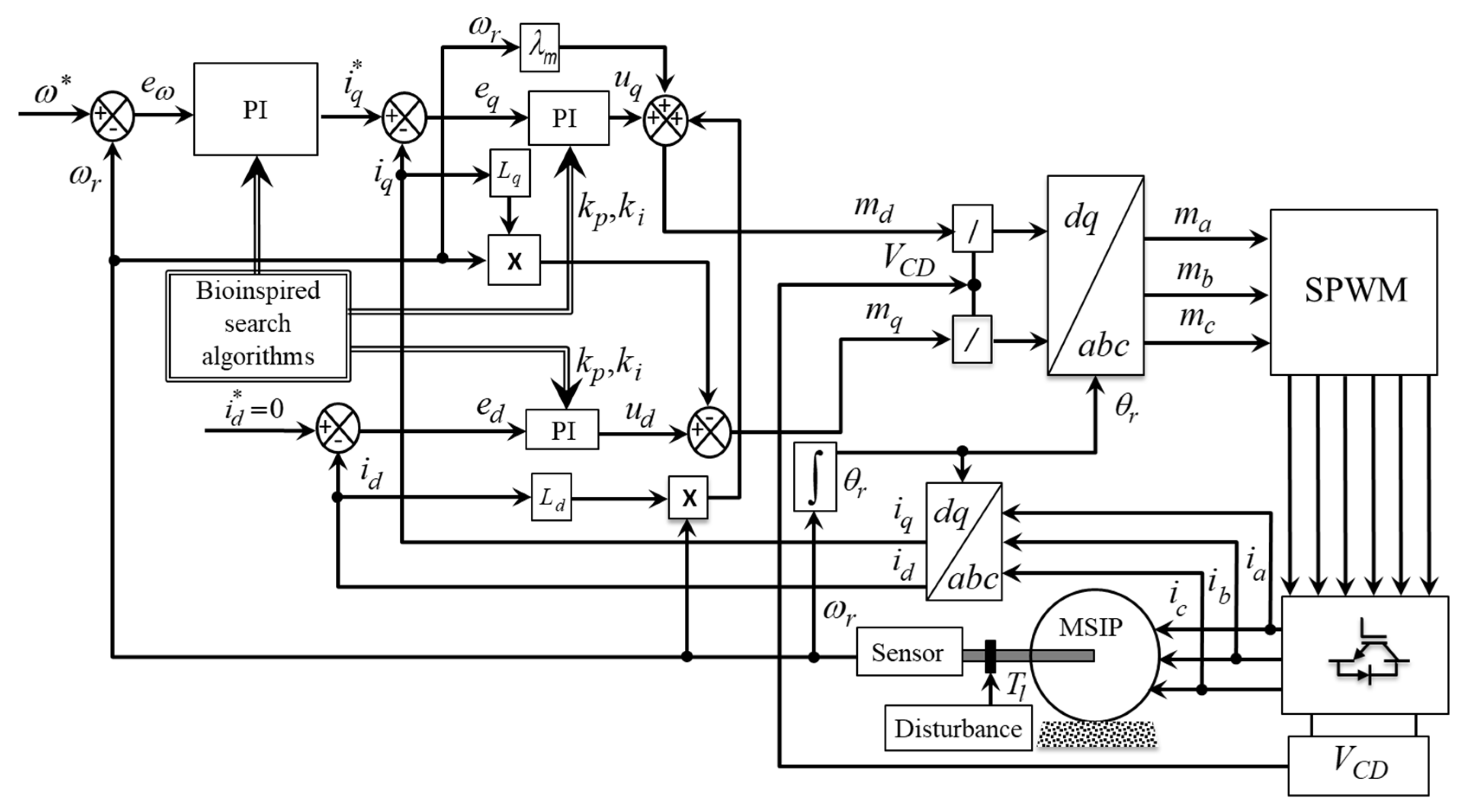
The purpose of this paper is to compare five different nature inspired algorithms to adjust the parameters of the PI controllers in order to determine which provides better performance when applied to the speed control of a PMSM. Algorithms inspired by the nature of BA, BBO, CSA, FPA and SCA are tested and the result is compared to show which one is more useful for speed regulation tasks. In summary, nature inspired algorithms search six gains for the speed tracking of a PMSM. The control system is based on three PI controllers where the gains are tuned using nature-inspired algorithms. The external PI control loop regulates the rotor speed to the desired reference value and sets the reference values for the internal control loop which regulates the currents on the d-axis and q-axis of the PMSM (Figure 1). The internal control loop consists of two PI controllers whose tasks are to regulate the i_q current to the value set by the external control loop and keep the i_d current equal to zero.

It is important to note that these optimization algorithms are increasingly popular in engineering applications because: (I) they are based on fairly simple concepts and are easy to implement; (II) they do not require gradient information; (III) they can overlook local optimals; (IV) they can be used in a wide range of problems spanning different disciplines.

2. Mathematical Model of PMSM

The PMSM is a nonlinear system, strong coupling between its mechanical and electrical variables. The differential equations that define the dynamics of the motor in a frame of reference dq can be defined as:

$$\frac{d{i}_d}{dt}=-\frac{R_s}{L_d}{i}_d+\frac{P{L}_q}{L_d}{i}_q\omega +\frac{1}{L_d}{u}_d$$

(1)

$$\frac{d{i}_q}{dt}=-\frac{R_s}{L_q}{i}_q-\frac{P{L}_d}{L_q}{i}_d\omega -\frac{P{\lambda }_m}{L_q}\omega +\frac{1}{L_q}{u}_q$$

(2)

$$\frac{d\omega }{dt}=\frac{1.5P{\lambda }_m}{J}{i}_q-\frac{b}{J}\omega -\frac{1}{J}{T}_l$$

(3)

where $i_d$, $i_q$, $u_d$ and $u_q$, are dq components of the current and the voltage in the stator respectively, $R_s$ is the stator resistance, $P$ is the number of pole pairs, ${\lambda }_m$ is the flux generated by the permanent magnet of the rotor, $L_d$ and $L_q$ are the dq components of the stator winding inductance, $b$ is a viscous damping coefficient, $J$ is the inertia moment and $T_l$ is the load torque. In case the PMSM is surface mounted permanent magnet type, $L_q$ is equal $L_d$, consequently, the electromagnetic torque $T_e$ can be defined as follows:

$$T_e=1.5\frac{n_p}{2}{\lambda }_m{i}_q$$

(4)

where n_p is the number of poles. The dynamic equations of the mechanical variables of the PMSM are expressed as

$$\frac{d{\omega }_r}{dt}=\frac{1}{J}\left(T_e-T_l\right)$$

(5)

$$\frac{d{\theta }_r}{dt}={\omega }_r$$

(6)

where ω_r is the mechanical speed of the rotor and, θ_r is the position of the rotor.

3. Control Scheme for PMSM

The control objective is to design an asymptotically stable speed controller for PMSM to make the rotor speed track the reference trajectory correctly under different parameter perturbations and load torque disturbances. Therefore, the main signal error can be defined as,

$$e_{\omega }={\omega }^{*}-{\omega }_r$$

(7)

where ω* is the desired rotor speed. If that the constant flow links have a linear relationship with the current in the stator; thereby its values can be estimate in an easy way. We can define the tracking error of the d-axis current as,

$$e_d=i_d^{*}-i_d$$

(8)

where $i_d^{*}$ is the d-axis current reference value. In theory, the proposed controller forces the current i_d to have a value of zero in a finite time, so that the electric torque is proportional to current i_q. Therefore, the current error in q-axis is defined as follows

$$e_q=i_q^{*}-i_q$$

(9)

where $i_q^{*}$ is the q-axis current reference value. The proposed control system is based on a sinusoidal pulse width modulation (SPWM) scheme; m_q and m_d are the modulating signals in dq reference frame. The modulation signals are transformed to abc system using the Park transformation and rotor position θ_r, for comparison with high-frequency carrier signal. Figure 1 details the control scheme.

4. Definition of the Tuning Problem Based on Optimization Algorithms

The problem to be solved in this work is a search for more optimal values for three PI controllers that regulate the rotor speed of the PMSM. To solve the optimization problem, it is necessary to use a target function to generate an adequate search space and find the best parameters of PI regulators. The objective function can be defined using different error criteria of the dynamic response of the system, such as: (a) Integrated absolute error (IAE), (b) Integrated Squared Error (ISE), (c) Integrated Time Squared Error (ITSE), (d) Integrated Time Absolute Error (ITAE). Although these definitions work properly, in this work we propose to use the following objective function [40], which allows us to obtain better results:

$$\min J=\left(1-e^{-\beta }\right)\left(M_p+e_{ss}\right)+e^{-\beta }\left(t_s-t_r\right)$$

(10)

where $M_p$ is the maximum overshoot; $e_{ss}$ is the error in steady state; $t_s$ is the time of establishment; $t_r$ is the rise time; and $\beta$ is the weighting factor that can be modified depending on the dynamic characteristics that are required to be reached. In relation to the objective function, Equation (10) the optimization problem can be defined as follows: minimize J subject to:

$$k_{p,j}^{min}\le k_p\le k_{p,j}^{max}$$

(11)

$$k_{i,j}^{min}\le k_i\le k_{i,j}^{max}$$

(12)

for j = [i_q, i_d, w]. It should be mentioned that β in (10) determines the magnitude of the characteristic values of the transient response of the system. If β > 0.7 is reduced M_P and e_ss; if β < 0.7 is minimized t_r and t_s. The search space of the parameters is defined as:

$$\begin{array}{cc}{k}_{p,i_q}=\left(0.01,300\right)& k_{i,i_q}=\left(0.01,50\right)\\ k_{p,i_d}=\left(0.01,180\right)& k_{i,i_d}=\left(0.01,150\right)\\ k_{p,{\omega }_r}=\left(0.01,500\right)& k_{i,{\omega }_r}=\left(0.01,350\right)\end{array}$$

The control scheme for PMSM is exposed in section three, however, a proper operation requires robust strategies or adaptive control that ensure safe and reliable performance also must respond quickly and appropriately to various scenarios that it may face.

5. Nature-Inspired Algorithms

The optimization process refers to finding the optimal values of the parameters of a given system from all possible values, in order to maximize or minimize its performance. Optimization problems can be found in all fields of study, which makes the development of optimization algorithms essential.

Optimization algorithms can be classified based on their nature as deterministic or stochastic algorithms. Deterministic algorithms follow a rigorous procedure, and its path and values of both design variables and functions are repeatable. Most conventional classical algorithms are deterministic, an example is the Newton Raphson algorithm.

Stochastic algorithms always have some randomness, the strings or solutions in the population will be different each time a program is executed because the algorithms use some pseudo-random numbers, the final results may not be very different, but the paths of each individual are not exactly equal. These algorithms are divided into two main groups: heuristic and metaheuristic.

The term heuristics means “to find or discover by trial and error”, using these algorithms quality solutions are found for a difficult optimization problem in a reasonable time, but there is no guarantee that optimal solutions will be reached. Metaheuristic algorithms generally work better than a simple heuristic, because these use some randomization trading and local search. It is worth noting that there are no agreed definitions of heuristics and metaheuristics in literature; some use “heuristics” and “metaheuristics” interchangeably [41].

Metaheuristics can be classified by their source of inspiration, most new algorithms today have been developed inspired by nature, most nature-inspired algorithms are based on some successful features of the biological system (biologically inspired, or bioinspired for short). Not all algorithms were based on biological systems, as many algorithms have been developed using the inspiration of physical, chemical and mathematical systems [42].

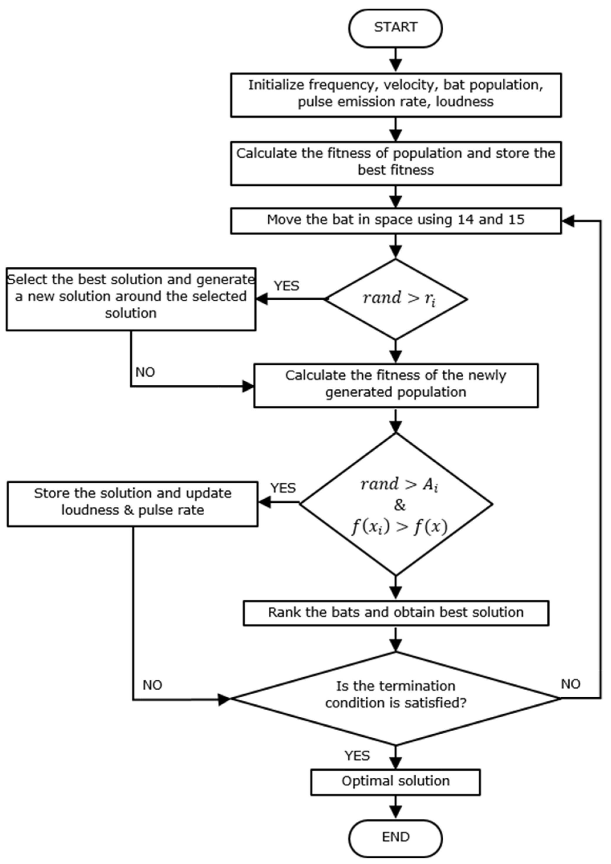
5.1. Bat Algorithm

The BA was developed by Yang [43] and mimics the behavior of small bats that use echolocation to orient themselves in the dark to avoid obstacles, detect prey and locate cracks. Echolocation is a navigation system based on the hearing of bats and some other animals to detect objects in their environment by emitting a sound signal to the environment.

Within the BA each virtual bat in the initial population employs a similar echolocation phenomenon to update its position. Bat echolocation is a perceptual system in which a series of strong ultrasonic waves are released to create echoes. These waves return with delays and at different audio levels, those bats evaluate to detect a specific prey. BA is based on the following rules that can summarize the behavior of bats using the echolocation process:

(a) Each bat uses the characteristics of the echolocation process to make a classification among its prey and obstacles.

(b) Bats fly randomly at an initial speed v_i to reach the initial position x_i; with a frequency that can vary from a minimum frequency f_min to a maximum frequency f_max; or varying the wavelength λ and its intensity or volume L to search for their prey. Bats can automatically adjust the wavelength or frequency of the signal they emit, and the number of pulses emitted r depends on how close your prey or target is.

(c) The intensity or volume changes from a high value L₀ to a constant minimum value L_min.

During the optimization process, the x_i position and v_i speed of each bat must be specified and updated in each BA iteration. The rules for obtaining new bat solutions and velocities are given by the following equations

$$f_i=f_{min}+\left(f_{max}-f_{min}\right)rand$$

(13)

$$v_i^{t+1}=v_i^t+\left(x^{*}-x_i^t\right)f_i$$

(14)

$$x_i^{t+1}=x_i^t+v_i^{t+1}$$

(15)

where $\mathrm{rand}\in [0,1]$ is a random vector that follows a normal distribution, $f_i$ is the frequency of the ith virtual bat, $f_{\min }$ and $f_{\max }$ is the minimum and maximum frequency that the bats will emit, respectively, $v_i^t$ and $v_i^{t+1}$ is the flight speed of the ith current bat and the next flight speed respectively, $x_i^t$ and $x_i^{t+1}$ is the position of the ith bat currently and at a later instant; y x* is the best solution currently generated, which is calculated by comparing all bat solutions. For the local search, a solution of all the best current solutions is chosen, a new solution for each bat is generated by means of a random path defined by the following expression

$$x_n=x_a+\epsilon L^t$$

(16)

where $x_n$ is the new solution, $x_a$ is the best old solution $\epsilon \in [-1,1]$, is a random number, $L^t$ is the average volume of all bats in iteration $t$. As the intensity is reduced if the bats are closer to their prey, while the number of emitted pulses is increased, the volume can be adjusted to a convenient value as follows

$$L_i^{t+1}=\alpha +L_i^t$$

(17)

$$r_i^{t+1}=r_i^0\left(1-e^{-\gamma t}\right)$$

(18)

where α is a random constant between 0 and 1, γ is a constant value greater than zero. The basic steps in the BA algorithm process are presented in the flowchart shown in Figure 2.

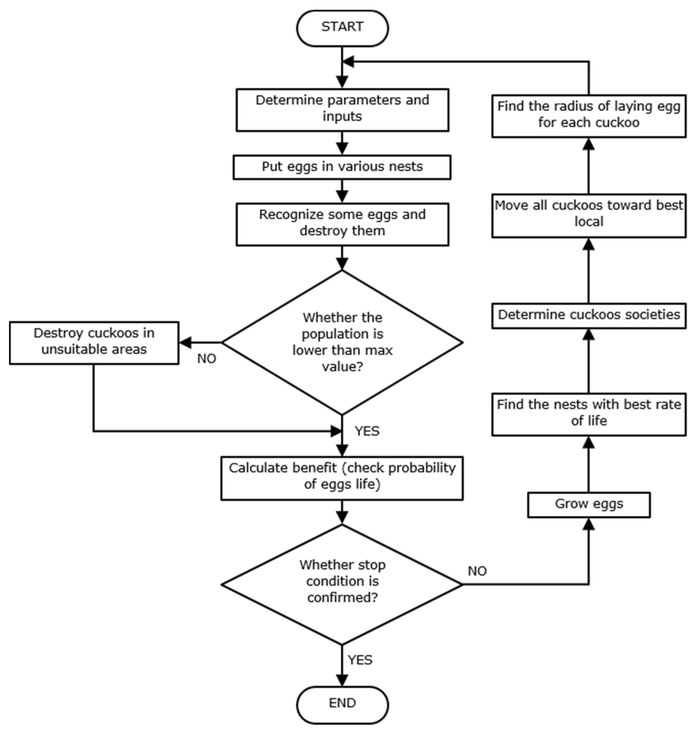
5.2. Cuckoo Search Algorithm

CSA is an algorithm based on the application of metaheuristics from nature. The CSA is an algorithm based on the aggressive breeding strategy of cuckoo birds and the Lévy flight characteristics of some bird species [44]. The CSA begins when the mother cuckoo lays her eggs in other people’s nests, of the same or another species of bird. The mother nest owner may discover that the eggs do not belong to her, so she may destroy the eggs or leave the nest with all the eggs inside.

Some species of cuckoo birds have evolved in such a way that the females throwing the eggs can imitate the color and pattern of the eggs of the selected nest. This action reduces the chance of the egg being abandoned and increases the ability to reproduce.

The cuckoo search algorithm can be described by the following three actions:

(a) Each cuckoo lays one egg at a time, which represents a set of coordinates of the solution and deposits it in a nest chosen at random.

(b) The part of the nests that contain the best eggs or candidate solutions is moved to form the next generation.

(c) The number of nests is fixed and sometimes the nest owner may discover a strange egg with a probability P_a ∈ [0, 1]. If this happens, the host may destroy the egg or leave the nest. This results in the construction of a new nest at a different location.

Using the above three rules, the CSA starts with an initial population randomly distributed to perform the search for a nest to lay the egg. The random position of the nest where the egg is laid is decided by making Levy flights, defined as:

$$x\left(t+1\right)=x\left(t\right)+\alpha \oplus Levy\left(\lambda \right)$$

(19)

where t is the current generation number and α > 0 is the step size. The product means input multiplications. Basically, Lévy flights provide a random walk, while their random steps are drawn from a Lévy distribution, which for large steps has an infinite variance with an infinite mean, with the form

$$Levy ~u=t^{-{\lambda }_c}, \left(-1<{\lambda }_c\le 3\right)$$

(20)

In the real world, if the egg of a cuckoo bird is very similar to the egg of the nest-owning bird, then the egg has less chance of being discovered so the suitability must be related to the difference in solutions. Following the rules defined above, the optimization algorithm can be summarized in the following flowchart (Figure 3).

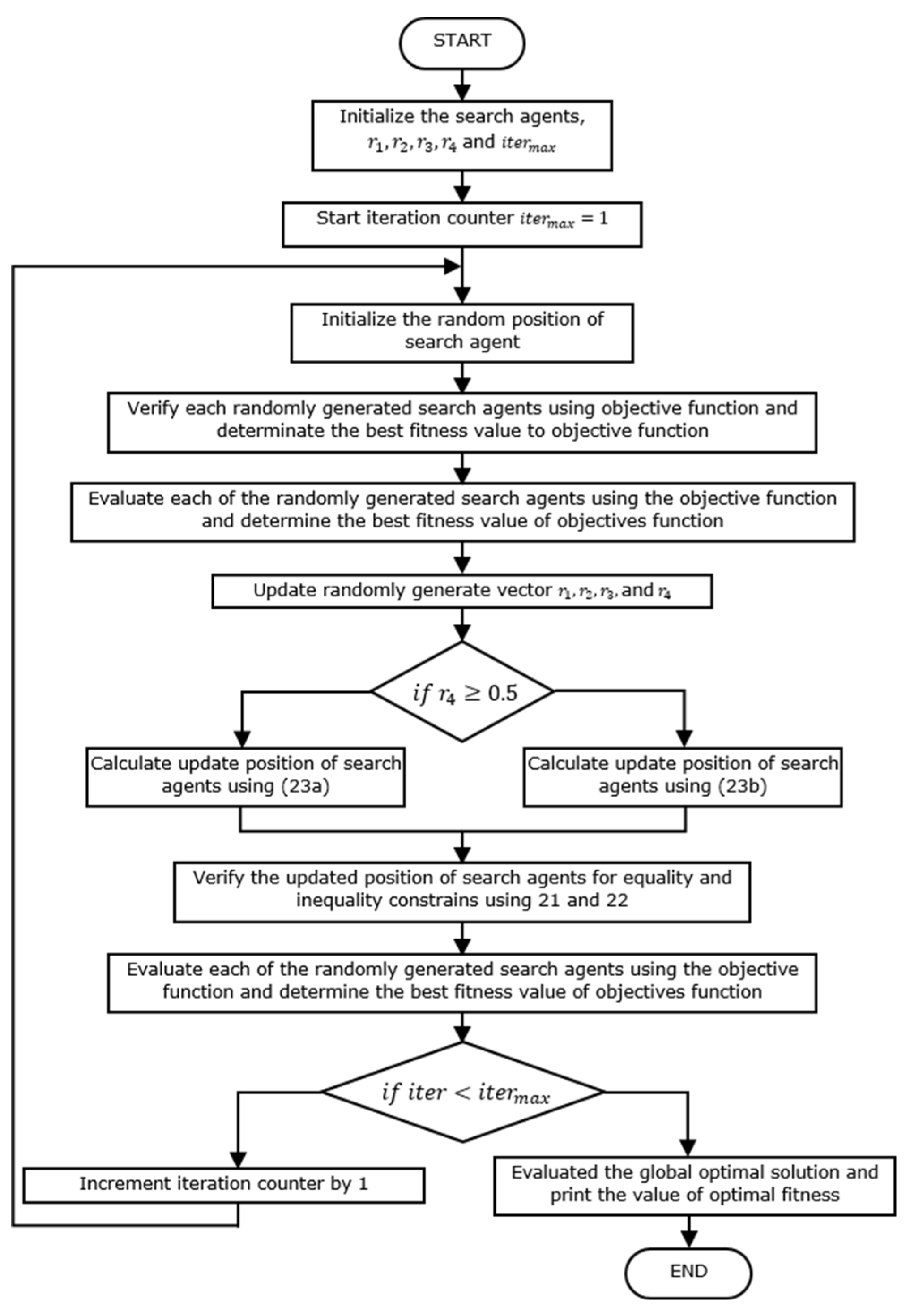
5.3. Sine-Cosine Algorithm

The sine cosine algorithm (SCA) is a new metaheuristic algorithm SCA is population based optimization technique that founds the optimization process with a set of random solutions [45]. These solutions are iteratively calculated over the course of iterations by an objective function. The probability of finding global optima is increased with the sufficient number of random solutions. The SCA is simply based on the Sine-Cosine function used for exploration and exploitation phases in optimization problems, which can be formulated as:

$$X_i^{t+1}=X_i^t+r_1\times \sin \left(r_2\right)\times \left|r_3{P}_i^t-X_i^t\right|$$

(21)

$$X_i^{t+1}=X_i^t+r_1\times \cos \left(r_2\right)\times \left|r_3{P}_i^t-X_i^t\right|$$

(22)

where $X_i^t$ is the location of current solution in i-th dimension at t-th iteration r₁, r₂, r₃ are random values, and P_i is the location of targeted optimal solution. The parameter r₁ is a control parameter that is decreased linearly from a constant value a to 0 by each iteration to achieve the balance between the exploration and exploitation phases of the algorithm Equations (21) and (22) are combined to be used for exploration and exploitation processes as follows:

$$X_i^{t+1}=\{\begin{array}{c}{X}_i^t+r_1\times \sin \left(r_2\right)\times \left|r_3{P}_i^t-X_i^t\right|, r_4<0.5\\ X_i^t+r_1\times \cos \left(r_2\right)\times \left|r_3{P}_i^t-X_i^t\right|, r_4\ge 0.5\end{array}$$

(23)

The designed parameter r₁ is employed to guide the next position’s region, which may be between the solution and destination or outside it. To achieve balance between exploration and exploitation phase, the dynamical fine-tune of r₁ during search process is carried out using Equation (24) as:

$$r_1=a-t\frac{a}{T}$$

(24)

where a is a constant, T is the maximum number of iterations and t is the current iteration. The r₂ is random variable which used to find the direction of the movement of the next solution (i.e., if it towards or outwards P_i). Also, the r₂ is random variable which gives random weights for P_i in order to stochastically emphasize (r₃ > 1) or deemphasize (r₃ < 1) the effect of desalination in defining the distance. The r₄ is a random number in [0, 1] is used to switch between the sine and cosine functions as in Equation (23). The steps of the SCA algorithm are given in Figure 4.

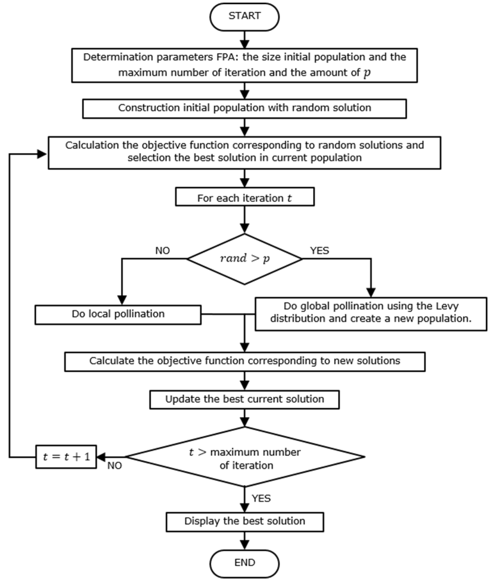
5.4. Flower Pollination Algorithm

Pollination is a natural mechanism for the reproduction of flowering plants and is defined as the transfer of pollen from one flower to the stigma of the pistil of the same flower or another flower of the same plant species. There are two types of pollination according to pollen transfer methods: (1) biotic pollination (90% of plants have this pollination) this is done by pollinators such as insects or animals. and (2) abiotic pollination (10% of plants have this pollination) does not require the transfer of pollen by living organisms, it is done by water, wind or gravity as pollinators. When pollen goes from one plant to another of the same type, such pollination is called cross-pollination and self-pollination occurs when pollen is delivered to the same flower or flowers of the same plant.

Generally, the size of the flowers is consistent with the bodies of the insects so that the insects can enter the flowers and their bodies are in contact with the pollen and pistil. Pollinating insects are often associated with a specific type of flower, which is defined as the constancy of the flower. That is, pollinators tend to sit on certain species of flowers. Therefore, flower constancy helps to quantify the cost of searching for each of the pollinators. For biotic pollination, pollinators such as flies, birds, and bats can fly long distances. Therefore, they can be considered as global pollination. Similarly, the passage jump or flight of birds or bees can be described as a collection flight. The strategies of biotic pollination, cross-pollination, abiotic pollination and self-pollination are defined in the domain optimization and incorporated in the flower pollination algorithm. The pollination process includes a series of complex mechanisms in plant production strategies. A flower and its pollen gametes form a solution to the optimization problem. The constancy of the flower as an adjusted solution is perceptible. In global pollination, pollinators transfer pollen over long distances to high adaptation. On the other hand, local pollination within a limited area of a single flower takes place under the shade of wind or water. Global pollination occurs with a probability called change probability. If this step is removed, then local pollination replaces it [23].

Four rules are followed in the FPA algorithm:

• Biotic pollination and cross-pollination are considered global pollination and pollen transporters or pollinators move in a way that follows Lévy flights.
• Abiotics and self-pollination are considered local pollination.
• Pollinators, including insects, can develop a floral constancy. Flower constancy is a production probability that is proportional to the similarity of two flowers involved.
• The interaction of global and local pollination can be controlled by the probability of change.

The first and third rules can be expressed as:

$$x_i^{t+1}=x_i^t+\gamma \times L\left(\lambda \right)\times \left(g_{*}-x_i^t\right)$$

(25)

where $x_i^t$ is the pollen or solution vector in iteration t; g_* is the best solution of all the generation of current solutions; γ is a scale factor to control the step isize and L is the pollination force, which is a step size related to the Lévy distribution.

Levy flight is a group of random processes in which the length of each jump follows Levy’s probability distribution function and has infinite variation. Following, L for a Levy distribution is given by:

$$L\approx \frac{\lambda \times \Gamma \left(\lambda \right)\times sin\frac{\pi \lambda }{2}}{\pi }\times \frac{1}{S^{1+\lambda }}S\gg S_{0}0,$$

(26)

where Γ(λ) is a standard range function.

For pollination, the second and third rule is given by

$$x_i^{t+1}=x_i^t+\epsilon \left(x_j^t-x_k^t\right)$$

(27)

where $x_j^t$ y $x_k^t$ are pollens from different flowers of the same plant species. This essentially imitates the constancy of the flower in a limited neighborhood. Mathematically, if $x_j^t$ y $x_k^t$ come from the same species or are selected from the same population, this becomes a local random walk if we extract $\in$ from a uniform distribution in [0, 1].

Most flower pollination activities can occur on both a local and global scale. In practice, adjacent flower patches or flowers in the not-so-distant neighborhood are more likely to be pollinated by local flower pollen than those that are far away. For this, we use a change probability (Rule 4) or a proximity probability p to switch between global pollination common to intensive local pollination.

Figure 5 represents the flowchart of the FPA algorithm that provides information on the execution steps of the optimization technique.

5.5. Biogeography-Based Optimization Algorithm

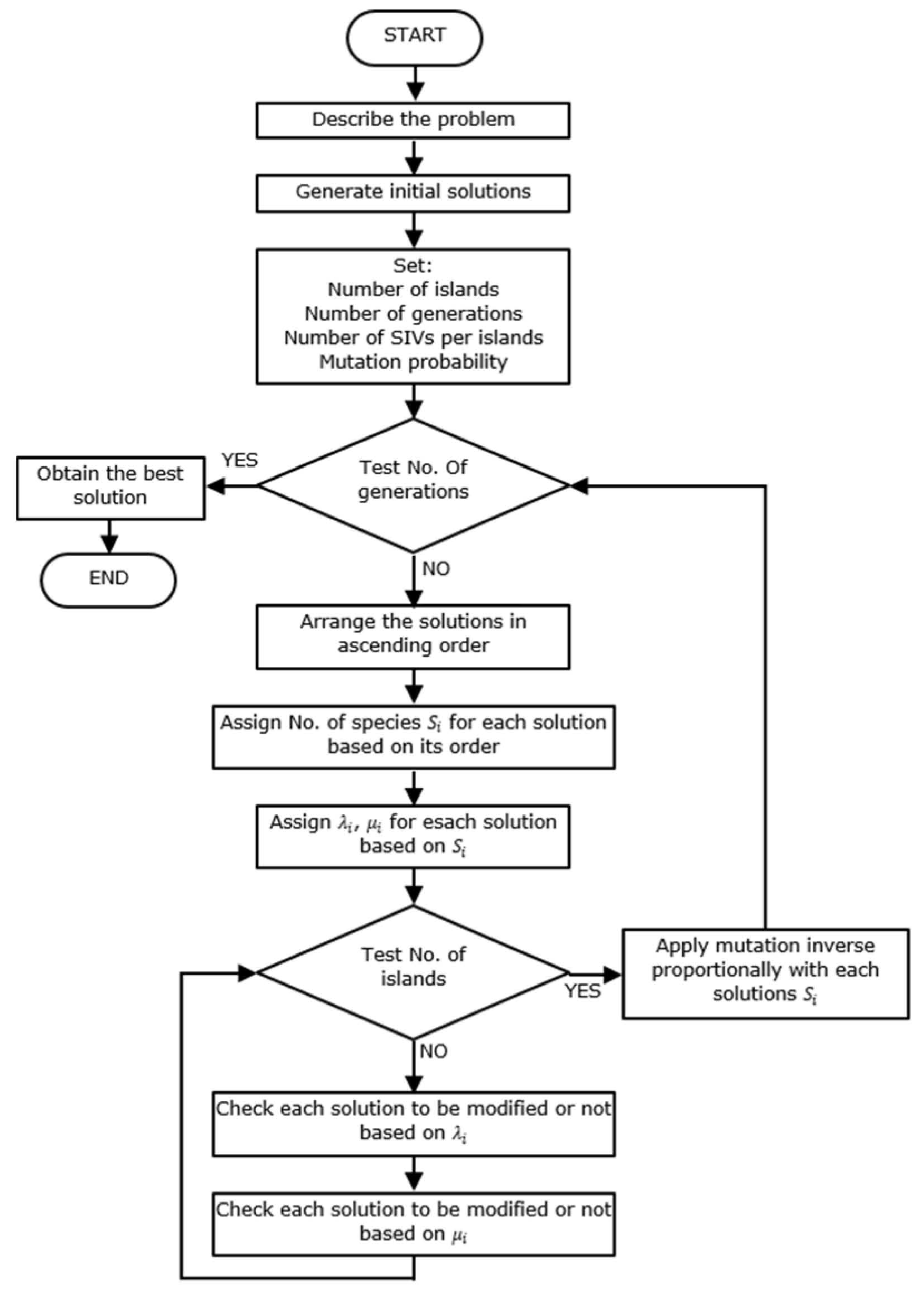
Inspired by biogeography, Simon developed a new approach called Biogeography-Based Optimization (BBO) in 2008. This algorithm is an example of how a natural process can be modeled to solve optimization [14]. In BBO, each possible solution is an island and their features that describe habitability are included in a Habitat Suitability Index (HSI). The goodness of each solution are named Suitability Index Variables (SIV). For example, of the natural process, why some islands may lean towards accumulating many more species than others. Because of possess certain environmental features that are more suitable to sustaining that kind than other islands with fewer species. It is axiomatic the habitats with high HSI have large populations and a high immigration rate and feature of a large number of species that migrate to other habitats. The rate of immigration will be lower if these habitats are already saturated with species. On the other hand, habitats with low HSI have high immigration and low immigration rate, because of the sparse population.

The fitness function FF is associated with each solution of Biogeography-Based Optimization BBO, which is analogous to HSI of a habitat. A good solution is analogous to a habitat having high HSI and a poor solution represents a habitat having a low HSI. The best solutions share their geographies of the lowest solutions throw migration (emigration and immigration). The best solutions have more resistance to change than the lowest solutions. However, the lowest solutions have more change from time to time and accept many new features from the best solutions. The immigration rate and emigration rate of the j-th island may be formulated as follows in Equations (28) and (29) [22].

$${\lambda }_i=I\left(1-\frac{j}{n}\right)$$

(28)

$${\mu }_i=\frac{E.j}{n}$$

(29)

where: μ_i, λ_i are the immigration rate and the emigration rate of j individual; I is the maximum possible immigration rate; E is the maximum possible emigration rate; j is the number of species of j-th individual; and is the maximum number of species. j-th in BBO, the mutation is used to increase the diversity of the population to get the best solutions.

Mutation operator modifies a habitat’s SIV randomly based on mutation rate. The mutation rate m_j is expressed in Equation (30).

$$m_j=m_{max}\left(\frac{1-p_j}{p_{max}}\right)$$

(30)

where m_j is the mutation rate for the j-th habitat having a j number of species; m_max is the maximum mutation rate; p_max is the maximum species count probability; p_j the species count probability for the j-th habitat and is given by Equation (31):

$$X_i^{t+1}=\{\begin{array}{c}-({\lambda }_i+{\mu }_i)P_j+{\mu }_i{P}_j,j\le 0\\ -({\lambda }_i+{\mu }_i)P_j+{\lambda }_{j-1}{P}_{j-1}+{\mu }_{j+1}{P}_{j+1},1\le j\le n\\ -({\lambda }_i+{\mu }_i)P_j+{\lambda }_{j-1}{P}_{j-1}+,j\le n\end{array}$$

(31)

where ${\mu }_{j+1}$, ${\lambda }_{j+1}$ are the immigration and emigration rate for the j-th habitat contains j + 1 species; ${\mu }_{j-1}$, ${\lambda }_{j-1}$, are the immigration and emigration rate for the j-th habitat contains j − 1 species. Figure 6 represents the flowchart of the BBO.

6. Results and Discussion

The adjustment parameters of the algorithms, which were used for the BBO are number of habitats equal to 40, a permanence range of 1 and a mutation factor of 0.04 [46]. For SCA was set maximum of iterations equal to 40 and 40 search agents, r₁ = 2 − (0.2t), r₂, r₃ and r₄ with a randomized value [45]. While CSA occupied the parameters 40 nests and a probability of finding foreign eggs P_a = 0.25 [25], the adjustment of the FPA are as size of population equal to 40, a maximum number of iterations equal to 40 and initial value of p equal to 0.8 [47], and BA with r₀ = 0.1, L₀ = 0.9, γ = 0.9, α = 0.9, F_min = 0 and F_max = 0 [43]. The initial population and the number of iterations for all the algorithms was fixed at 40, the same value was chosen so that the results could be object of comparison, the parameters of each algorithm are taken from the referenced articles.

Obtaining the gains of the three PI controllers that make up the speed control scheme occurs based on simulations developed in the Matlab environment, where the different heuristics and the dynamic model of the PMSM described by the differential Equations (1)–(3) are integrated.

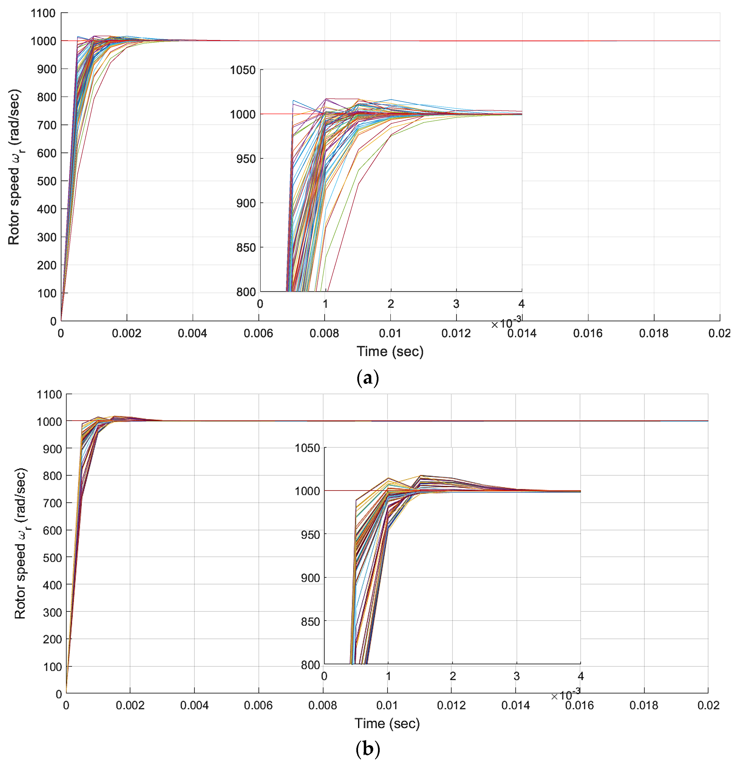
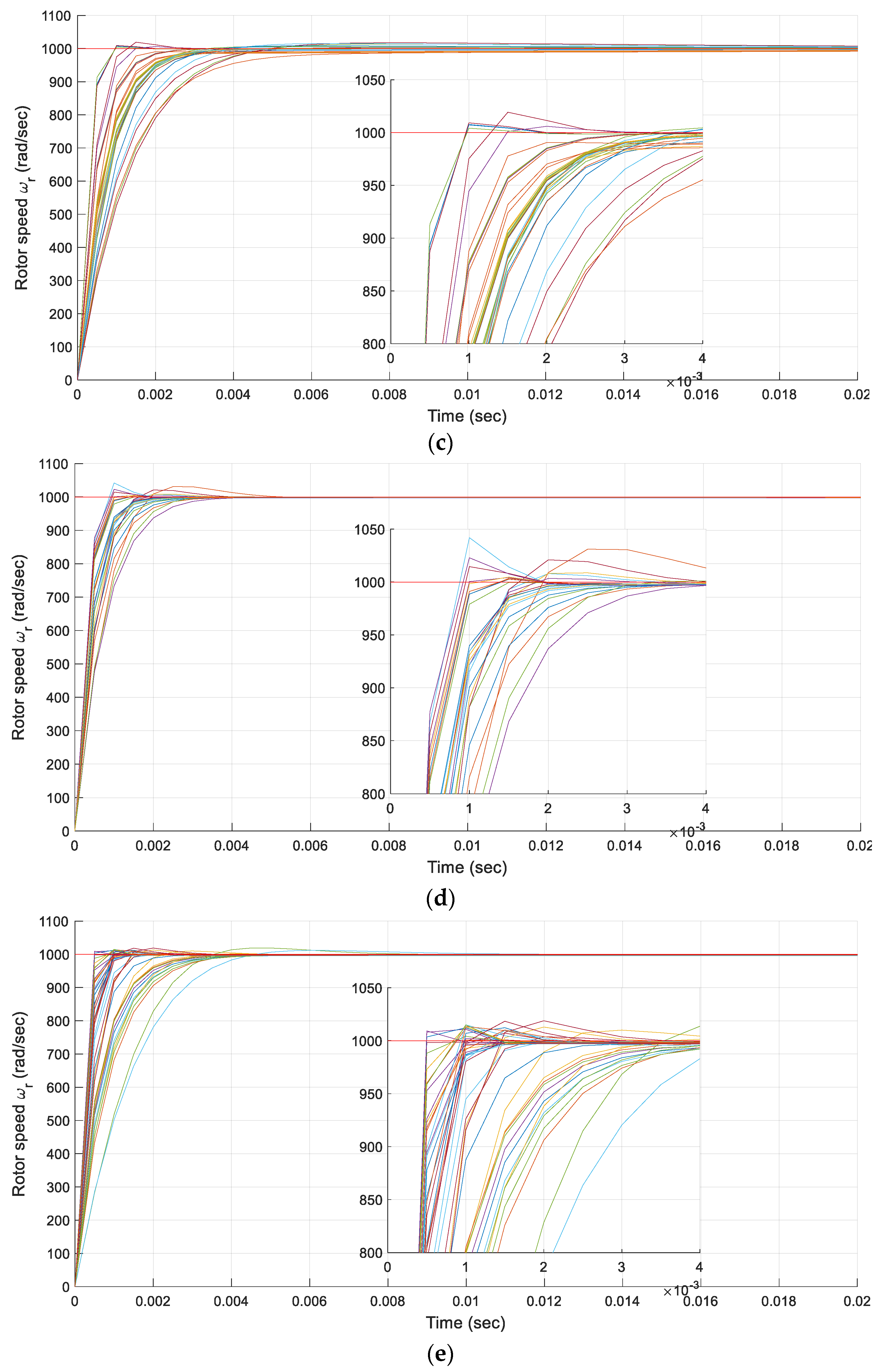
The motor parameters used in the simulation are contained in

Table 1. Parameters of PMSM.

Parameter	Symbol	Value and Units
Inertia moment	$J$	3.5 × 10−5 Nm
Nominal voltage	$v$	200 V
Stator resistance	$r_s$	2.6 Ω
Stator inductance d	$L_d$	6.73 mH
Stator inductance q	$L_q$	6.73 mH
Magnetic flux	${\lambda }_m$	0.319 Wb
Pole pairs	$n_p$	4

. While the graphs in Figure 7 show the behavior of the system using the different algorithms, feeding with a step (1000 rad/s), and under constant load torque (1 Nm).

The results of single run might be unreliable due to the stochastic nature of meta-heuristics. All of the algorithms are run 25 times and statistical results from the evaluation of the gains of the three PI controllers, calculated by the different optimization algorithms in the control the PMSM (minimum, maximum, mean and standard deviation) are collected and reported in

Table 2. Minimum function statistical data using different optimization algorithms.

Algorithm	Min	Max	Mean	Std
FPA	1.7518	11.9437	5.93158	2.9066
BBO	10.1006	22.3857	13.0411	3.4514
BA	10.9315	32.5701	18.1538	6.3145
CSA	10.4840	15.2290	12.0131	1.2182
SCA	10.2420	14.0670	11.49813	1.3842

. These results show that the FPA managed to obtain the smallest value of the minimum function, with the BBO being the second best, followed by SCA and CSA, with BA presenting the worst result.

The gains of PI controllers found through BA, FPA, SCA, CSA and BBO are listed in

Table 3. Optimal gains for PI controllers.

Algorithm	${\mathit{k}}_{\mathit{p}},\mathsf{\omega }$	${\mathit{k}}_{\mathit{i}},\mathsf{\omega }$	${\mathit{k}}_{\mathit{p}}$$,{\mathit{i}}_{\mathit{q}}$	${\mathit{k}}_{\mathit{i}}$$,{\mathit{i}}_{\mathit{q}}$	${\mathit{k}}_{\mathit{p}}$$,{\mathit{i}}_{\mathit{d}}$	${\mathit{k}}_{\mathit{i}}$$,{\mathit{i}}_{\mathit{d}}$
FPA	0.2252	9.7873	6.7903	12.1943	2.6506	8.5429
BBO	0.3274	18.4462	9.7514	19.2666	19.0868	10.9512
BA	0.3449	18.2279	9.1039	25.0000	31.3601	13.1409
CSA	0.3460	17.0000	9.0940	3.4042	6.9401	4.1019
SCA	0.3158	17.0000	9.6341	1.9076	0.1152	4.6480

. The tests were performed on PC with Intel (R) Core (TM) i7-7500U 2.9 GHz with 8.00 GB in RAM and with 2016b version of Matlab.

The execution time of the different algorithms for the calculation of the profits of the PI controllers is shown in

Table 4. Execution time of optimization algorithms.

Algorithm	Average Running Time (s)
FPA	7.7704
BBO	30.0921
BA	5.8327
CSA	5.1923
SCA	5.2713

.

In order to know the performance of controllers in operating conditions where an unknown variable load torque is presented, the load torque is modeled using a Lorenz system described by the following first-order differential equations.

$$\frac{dx}{dt}=a\left(y-x\right)$$

(32)

$$\frac{dy}{dt}=x\left(b-z\right)-y$$

(33)

$$\frac{dz}{dt}=xy-cz$$

(34)

$$T_l=0.04z$$

(35)

where a = 5, b = 12y, c = 25; with initial conditions: x(0) = 0.1, y(0) = 0.1 and z(0) = 0.5 [48]. Below are two cases in which the reference trajectory has different natures. In the first case the transition between the desired speed values is smooth. In the second case the changes in the reference speed are values with a constant rate of change defined by slopes.

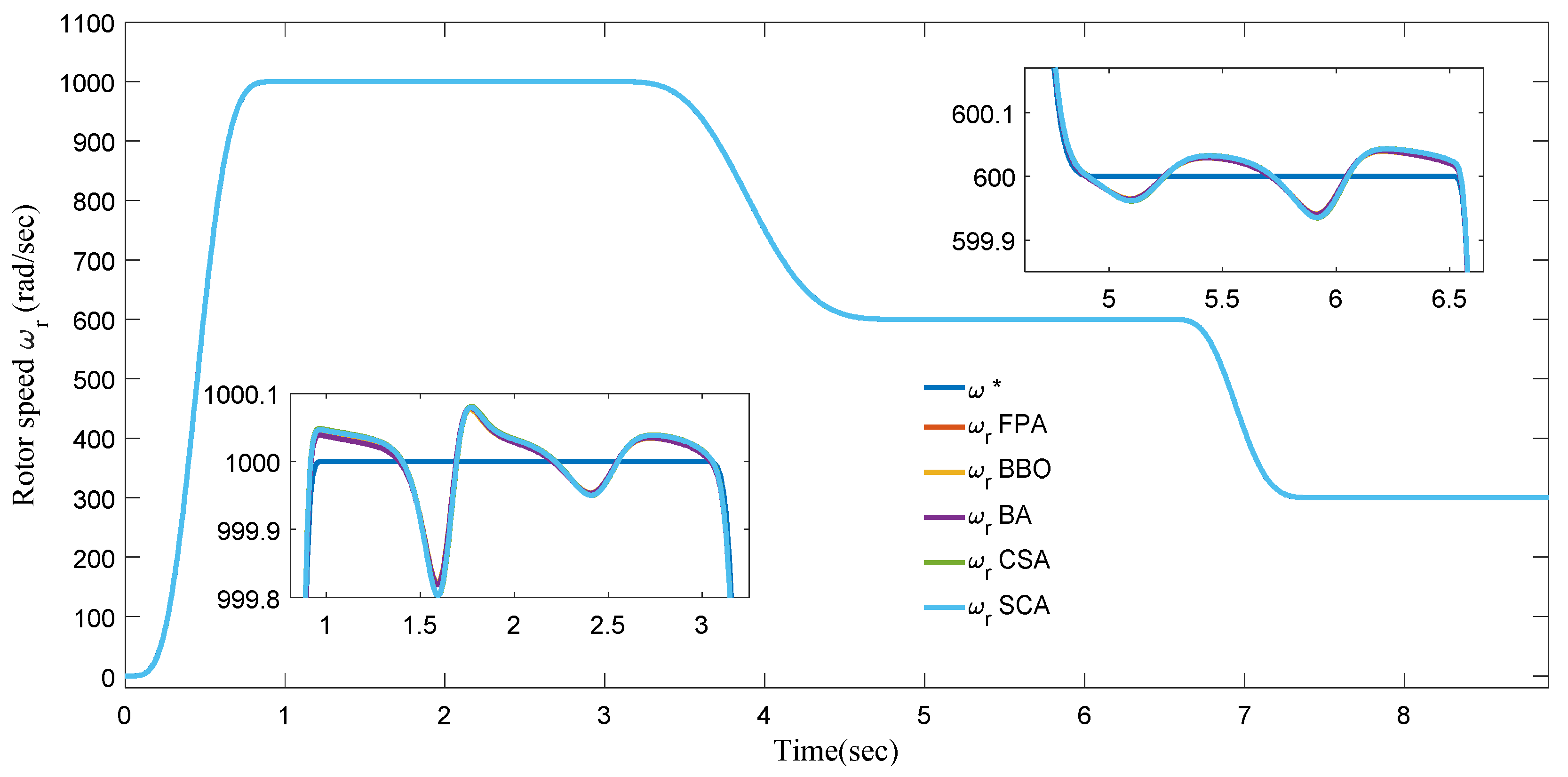
6.1. Case 1 PMSM Response to a Speed Reference Characterized by Bezier Polynomials with Variable Load Torque

The reference speed is given by a Bézier polynomial ψ for providing a sufficiently smooth transfer between the actual and desired speed reference values, within a specific time interval. Then, the reference trajectory is as follows [49]

$${\omega }^{*}=\{\begin{array}{cc}{\omega }_1+({\omega }_2-{\omega }_1)\psi (t,T_1,T_2)& for T_1\le t\le T_2\\ {\omega }_1& for T_2\le t\le T_3\\ {\omega }_1+({\omega }_2-{\omega }_1)\psi (t,T_3,T_4)& for T_3\le t\le T_4\\ {\omega }_2& for T_4\le t\le T_5\\ {\omega }_1+({\omega }_3-{\omega }_2)\psi (t,T_5,T_6)& for T_5\le t\le T_6\\ {\omega }_3& for t>T_6\end{array}$$

(36)

where ω₁ = 1000 rad/s, ω₂ = 600 rad/s, ω₃ = 300 rad/s, T₁ = 0 s, T₂ = 1 s, T₃ = 3 s, T₄ = 5 s, T₅ = 6.5 s y T ₆ = 7.50 s, and ψ is a polynomial function with the form

$$\psi =K^5\left[r_1-r_{2}K+r_3{K}^2-r_4{K}^3+\dots -r_6{K}^5\right]$$

(37)

$$K=\frac{t+T_i}{T_f-T_i},\mathrm{for}i=1,2,3,4$$

(38)

The performance of the controllers is verified using performance indices such as ISE, IAE, ITSE and ITAE. The ISE penalizes the controller for steady state errors, while IAE penalizes the controller for transient errors, ITSE penalizes the controller for steady state errors over a prolonged time and ITAE penalizes the controller for transient state errors over a prolonged time.

Table 5. Performance indices of PI controllers tuned using BA, BBO, CSA, FPA and SCA in case 1.

Algorithm	ISE	IAE	ITSE	ITAE
FPA	0.0692	0.4489	0.1122	1.6248
BBO	0.0681	0.4445	0.1095	1.6036
BA	0.0697	0.4494	0.1126	1.6251
CSA	0.0824	0.4925	0.1340	1.7851
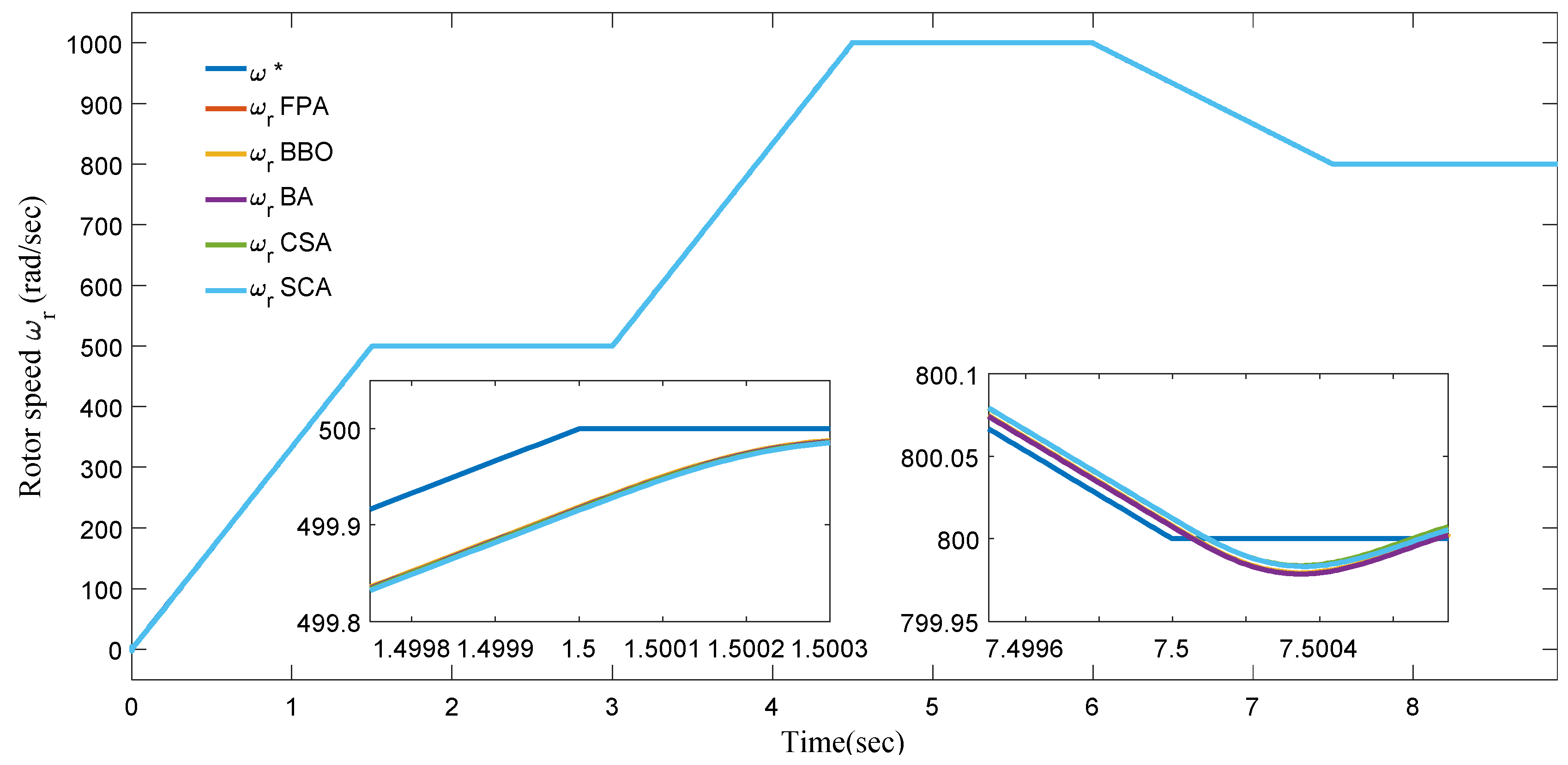
SCA	0.0820	0.4886	0.1318	1.7697

shows these indicators for case 1. The smallest indicators are the result of the BBO algorithm, presenting the best performance in speed tracking, followed by the FPA, BA, SCA algorithms and with the largest amount of error for the CSA.

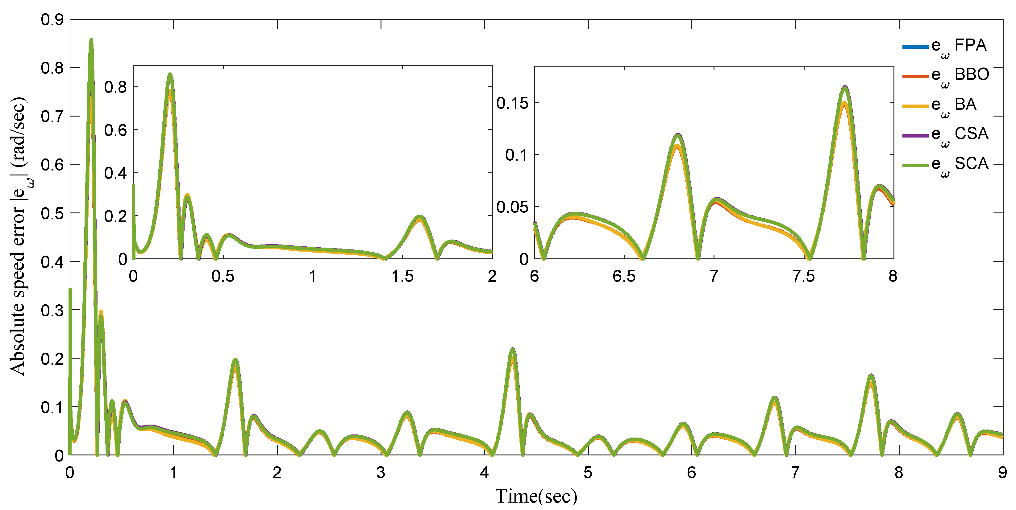
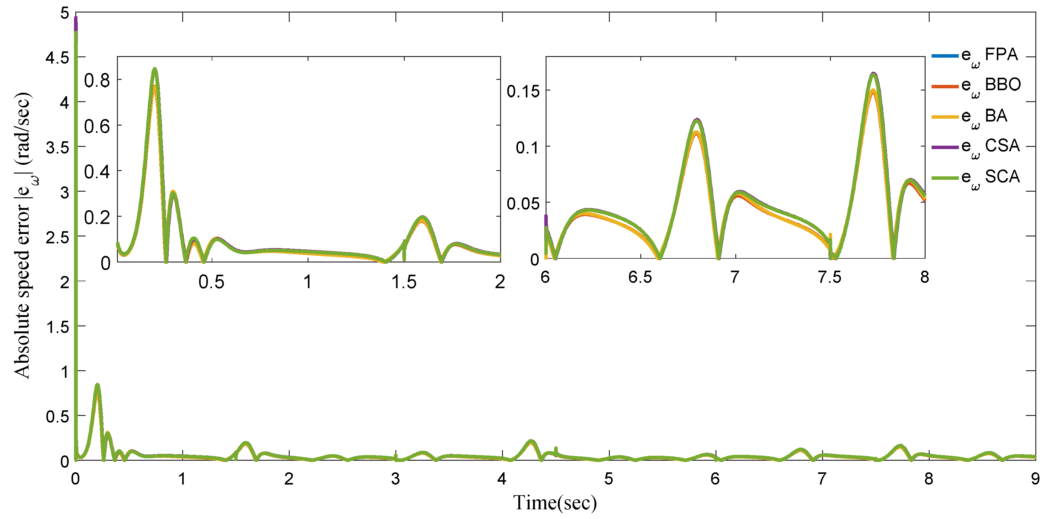
Figure 8 show the speed tracking of all algorithms for case 1, where there is an error in steady state less than 0.001% of the nominal reference value, it can be observed that the different algorithms achieve the appropriate tracking of the desired speed profile. The absolute error is shown in Figure 9, being the maximum error of just 0.9 rad/s, being the BBO the algorithm that gives the least error and CSA the one that gives the greatest error.

6.2. Case 2 PMSM Response to a Trapezoidal Speed Reference with Variable Load Torque

The speed references given by a series of trapezoidal shapes, where the change of reference values depends on the slope of the waveform. Then, the reference trajectory is as follows

$${\omega }^{*}=\{\begin{array}{cc}(\frac{{\omega }_2-{\omega }_1}{T_2-T_1}\times t)+{\omega }_1& for T_1\le t\le T_2\\ {\omega }_2& for T_2\le t\le T_3\\ (\frac{{\omega }_4-{\omega }_3}{T_4-T_3}\times t)-{\omega }_3& for T_3\le t\le T_4\\ {\omega }_4& for T_4\le t\le T_5\\ (\frac{{\omega }_6-{\omega }_5}{T_6-T_5}\times t)+({\omega }_6+{\omega }_5)& for T_5\le t\le T_6\\ {\omega }_6& for t>6\end{array}$$

(39)

where ω₁ = 0 rad/s, ω₂ = 500 rad/s, ω₂ = ω₃, ω₄ = 1000 rad/s, ω₄ = ω₅, ω₆ = 800 rad/s, T₁ = 0 s, T₂ = 1.5 s, T₃ = 3 s, T₄ = 4.5 s, T₅ = 6 s and T₆ = 7.5 s.

Figure 10 shows the speed tracking of all algorithms for case 2, the speed behavior is shown when the path changes from a slope-dependent value to a constant value. The absolute error is shown in Figure 11, where unlike case 1, the initial error is greater because this path is not as smooth. As in case 1 the best result is obtained using the BBO and the algorithm with the largest error is CSA.

Table 6. Performance indices of PI controllers tuned using BA, BBO, CSA, FPA and SCA in case 2.

Algorithm	ISE	IAE	ITSE	ITAE
FPA	0.0803	0.4513	0.1133	1.6335
BBO	0.0784	0.4462	0.11036	1.6120
BA	0.0804	0.4515	0.1134	1.6338
CSA	0.0928	0.4938	0.1349	1.7937
SCA	0.0915	0.4896	0.1328	1.7781

shows performance indicators ISE, IAE, ITSE and ITAE for case 2, sorting these algorithms in ascending order according to the smallest error we first have the BBO, followed by FPA, BA, SCA and lastly CSA.

The results shown prove the usefulness and good performance of nature inspired algorithms. The tests carried out with the gains of the PI controllers calculated for the speed control show that the algorithms have a similar behavior since everyone complies with the tracking of the reference speed trajectory, only highlighting the BBO algorithm as the one that has a minor error.

7. Conclusions

In this work we compare optimization algorithms based on nature to tune three PI controllers that regulate the rotor speed of a PMSM. Four algorithms inspired by nature: BA, BBO, CSA and FPA and one algorithm inspired by the mathematical function SCA were taken into account to make the most optimal search for gains.

The results of the simulations show that the five algorithms used to tune the parameters of the PI controllers work well to follow different trajectories with variable or constant load torque. By comparing the response of each of the algorithms in the two proposed cases, and based on the different error indicators (Table 5; Table 6) it can be concluded that the BBO works best under different operating conditions. It is worth mentioning that the gains were calculated in conditions of constant load torque and constant speed. Under these conditions, the algorithm that showed the best performance was the FPA, having the smallest minimum function and the smallest average among all the algorithms as can be seen in Table 3, situation that changed when having a variable load torque. Future research should focus on improving the response of these algorithms to disturbances, uncertainties and parametric variations.

Future works consist of the application of different algorithms inspired by nature to calculate and optimize PID controller gains for others electric machines. Experimental results on optimized PID controller combined with adaptive control in electromechanical energy conversion systems will also be introduced in subsequent studies. Another research line will involve testing the response of more complex industrial plants when using other bio-inspired and intelligent techniques. In the same way, a statistical analysis will be included to determine the significance of the results. The final research goal will include the experimental validation of this paper.