Parameterized Algorithms in Bioinformatics: An Overview

Abstract

Bioinformatics regularly poses new challenges to algorithm engineers and theoretical computer scientists. This work surveys recent developments of parameterized algorithms and complexity for important NP-hard problems in bioinformatics. We cover sequence assembly and analysis, genome comparison and completion, and haplotyping and phylogenetics. Aside from reporting the state of the art, we give challenges and open problems for each topic.

1. Introduction

With the dawn of molecular biology came the need for biologists to process and analyze data way over human capacity, implying the need for computer programs to assemble sequences, measure genomic distances, spot (exceptions to) patterns, and build and compare phylogenetic relationships, to name only few examples. While many of these problems have efficient solutions, others are inherently hard. In this work, we survey selected NP-hard problems in genome comparison and completion (Section 2), sequence assembly and analysis (Section 3), haplotyping (Section 4), and phylogenetics (Section 5), along with important results regarding parameterized algorithms and hardness. While trying to be accessible to a large audience, we assume that the reader is somewhat familiar with common notions of algorithms and fixed-parameter tractability, such as the $O^{*}(.)$-notation, giving only exponential parts of a running time, ignoring polynomial factors (for details about parameterized complexity, we refer to the recent monographs [1,2]). In a nutshell, parameterized complexity exploits the fact that the really hard instances are pathological and real-world processes generate data which, although enormous in size, are very structured and governed by simple processes. It seems straightforward that biological datasets abide by this “law of low real-world complexity”.

While excellent surveys of fixed-parameter tractable (FPT) problems in bioinformatics exist [3,4,5,6], this work tries to present an update, summarizing the state of the FPT-art as well as reporting on some additional “hot topics”. We further aim at: 1. iterating that parameterized algorithms are a viable and widespread tool to attack NP-hard problems in the context of biological data; and 2. supplying engineers and problem-solvers with computational problems that are actually being solved in practice, inspiring research on concrete open questions. Herein, we focus on problems that are particular for bioinformatics, avoiding more universal and general problems such as the various versions of Clustering which, while important for bioinformatics, have applications in many areas.

Generally, each topic has a problem description, a results section, some open problems and, possibly, an assortment of notes, giving additional information about less popular variants, often only mentioning results or problems related to the main topic without going into details. Finally, we want to apologize for the limited coverage of relevant work but, as our colleague Jesper Jansson wrote,

“Writing a survey about bioinformatics-related FPT results sounds like a monumental task!”

2. Genome Comparison and Completion

This section considers genetic data at its largest scale, i.e., as a sequence of genes, independent of their underlying DNA sequences. At this scale, long-range evolutionary events occur, cutting and pasting whole segments of chromosomes (“chromosomal rearrangement”) [7]. The number of such rearrangements between the genomes of two species can be used to estimate their “genetic distance” which, in turn, allows for phylogenetic reconstruction. Further, we consider the problems of identifying genes with a common ancestor after duplications, and filling the gaps in an incomplete genome.

In the most general setting, a genome G may be represented as a collection of strings and circular strings, where each string represents a chromosome and each character represents a gene or gene family. However, for ease of representation, most models use a single-sequence representation of the genome (which generalizes easily to multi chromosomal inputs in most cases). There is however an important distinction between the string model, allowing gene repetitions (also called duplicates, or paralogs), and the permutation model enforcing that each gene appears exactly once. Many problems in the following sections can be formulated in both models. The string model is obviously the most general in practice, but often comes with a prohibitive algorithmic cost. Parameterized algorithms can offer a good solution, using the fact that most genes only have a small number of occurrences. Thus, the maximum number of occurrences of any character in an input string, denoted occ in this paper, is a ubiquitous parameter. In both models, a genome is signed if each gene is given a sign (+ or −) representing its orientation along the DNA strand.

In the following, a string $s^{\prime }$ is called substring of a string s if $s^{\prime }=s$ or $s^{\prime }$ is the result of removing the first or last character of some substring of s. Further, $s^{\prime }$ is called subsequence of s if $s^{\prime }=s$ or $s^{\prime }$ is the result of removing any character from a subsequence of s. We say that two strings are balanced if each character appears with the same number of occurrences in both.

2.1. Genomic Distances

The problems in this section aim at computing a distance between genomes, reflecting the “amount of evolution” that occurred since the last common ancestor. Among the most basic distances for the permutation model is the breakpoint distance, counting the number of pairs of genes that occur consecutively in one genome but not in the other (a pair $\mathtt{ab}$ is considered to be identical to $\mathtt{ba}$ in the unsigned model, however $+\mathtt{a}+\mathtt{b}$ is identical only to $+\mathtt{a}+\mathtt{b}$ and $-\mathtt{b}-\mathtt{a}$ in the signed model). Its complement is a measure of similarity, the number of common adjacencies (the number of pairs of consecutive genes that occur in both genomes). Common adjacencies can easily be generalized in the string model: adjacencies of each genome are seen as a multi-set, and the number of common adjacencies is the size of the intersection of these multi-sets.

More advanced genomic distances are rearrangement distances. A rearrangement acts on the genome by reordering some genes in a certain way, mimicking a large-scale evolutionary event. The core question in rearrangement distances is to compute the minimum number of rearrangements transforming a genome into another. These distances are more precise—in the sense that they directly describe parsimonious evolutionary scenarios—but in most cases significantly more difficult to compute than the breakpoint distance. Note that balanced genomes are usually considered, i.e., any character appears with the same number of occurrences in every genome. See the work of Fertin et al. [8] for an extensive survey on rearrangement distances.

2.1.1. Double-Cut and Join Distance

Problem Description. The double-cut and join distance needs the most general genome model as intermediary steps, that is, a multi-set of strings and circular strings. A double-cut and join operation splits the genome in two positions and joins the four created endpoints in any way (see Figure 1). For signed genomes, this operation is required to maintain consistent orientation of each gene. We focus on the case where the source and target genomes have a single chromosome (i.e., strings or permutations).

Results. The DCJ distance can be computed in linear time in the signed permutations model [9,10]. However, it is NP-hard in the unsigned permutation or string models [11]. On the positive side, it admits an $O\left(2^{2k}n\right)$-time algorithm for unsigned permutations [12].

An issue with the DCJ distance is that the solution space might be very large, as many different scenarios may yield the same distance. Thus, more precise models have been designed to “focus” the solution towards the most realistic scenarios. Fertin et al. [13] introduced the wDCJ distance, where intergene distances are added to the genome model and must be accounted for in the DCJ scenario (when breaking between consecutive genes, the number of intergenomic bases must be shared among both sides). This variant makes the problem NP-hard for signed permutations, but fixed-parameter tractable for the parameter k. Another constraint focuses on common intervals, which are segments of the genomes that have exactly the same gene content, but in different orders. A DCJ scenario is perfect if it never breaks a common interval. Bérard et al. [14] showed that finding a perfect scenario with a minimum number of operations is FPT for a parameter given by the common interval structure.

2.1.2. Reversal Distance

Problem Description. A reversal [15] is a rearrangement reversing the order of the characters in any substring of the genome. When considering signed genomes, a reversal additionally switches all the signs in the reversed substring (see Figure 2).

Results. Sorting by Reversals is polynomial-time solvable in the signed-permutations model [16]. However, it is NP-hard for unsigned permutations [17] and for strings, even when occ = 2 [18] and for binary signed strings [19]. For unsigned permutations, Sorting by Reversals is easily FPT for k, using the fact that reversals never need to cut at positions that are not breakpoints [20]. For balanced strings, a possible parameter, $b_{max}$, is the number of blocks of the input strings, where a block is a maximal factor of the form ${\mathtt{a}}^n$ for some character $\mathtt{a}$. Sorting by Reversals can be solved in $O^{*}\left(b_{max}^{O\left(b_{max}\right)}\right)$ time in both the signed and unsigned variants [21]. As for DCJ, the variant restricting scenarios to reversals preserving common intervals is also NP-hard, and FPT for a parameter given by the common interval structure [22].

Notes. Other rearrangements can be considered, such as transpositions (two consecutive factors are swapped), and the prefix and/or suffix variants of reversals and transpositions (that is, reversals and transpositions affecting the first or last character of the sequence, respectively) (see, e.g., [23]).

No polynomial-time algorithm is known for computing these rearrangement distances, although NP-completeness is still open, notably on permutations for signed prefix reversals and prefix transpositions. Fixed-parameter tractability results may be achieved in the permutation model using the relationship between these rearrangements and breakpoints [24], and in the string model using the number of blocks $b_{max}$ as a parameter [21,25].

2.2. Common Partitions

Two strings $S_1$ and $S_2$ have a common string partition S if S is a (multi-)set of strings called blocks such that both $S_1$ and $S_2$ can be seen as the concatenation of the blocks of S. Furthermore, S is a common strip partition if each of its blocks has length at least two. Note that any two balanced strings have a common string partition, but may not have a common strip partition. Common strings or common strips may be used to identify syntenic regions between two genomes. Intuitively, most genes from the genomes of two close species should have a simple common string partition.

2.2.1. Minimum Common String Partition

Problem Description. The most natural partition problem is Minimum Common String Partition [18] (see Figure 3), which admits slightly different formulations [26,27]. It can be seen as a generalization of the breakpoint distance on balanced strings. Indeed, a common string partition may be seen as a mapping between the characters of both strings, i.e., a permutation, whose breakpoints correspond to the limits between consecutive blocks. Rather than a genomic distance, it can also be seen as a method for assigning orthologs across two genomes, assuming that all duplication events happened before their last common ancestor. For example, depending on how orthologs are matched, genomes abacd and acdab may be seen as permutations 12345 and 34512 (i.e., matching two blocks ab and acd), or 12345 and 14532 (matching four blocks a, b, a, and cd). Gene sequences alone may not be sufficient to distinguish both cases: in such a situation, the first option presumably reflects better the evolutionary history of these species, since it involves fewer large-scale events in the genome.

Results. MCSP is FPT for several combinations of parameters, depending on the relative size of the blocks, the size k of the partition and/or the maximum number occ of occurrences of a character  [28,29]. It can also be solved in $k^{O\left(k^2\right)}$ time [30], although this is too slow to be of practical interest. Finally, MCSP admits a more practical algorithm for the parameter $k+$ occ, running in O(occ^2kkn) time [31]. This last algorithm also applies to unbalanced strings where the problem is extended as follows: excessive characters may be removed from their respective input strings, but only between consecutive blocks.

Another possible parameter is the number of preserved duos, $k^{\prime }=\left|G_1\right|-k$. Note that MCSP is denoted Maximum-Duo Preserving String Mapping in the context of approximations and parameterized algorithms maximizing $k^{\prime }$. This version is FPT as well, and admits a kernel of size $O\left(k^{\prime 8}\right)$ [32].

2.2.2. Maximal Strip Recovery

Problem Description. In the Maximal Strip Recovery problem [33] (see Figure 4), the goal is again to identify common blocks between two genomes. But here, we may remove characters (genes) from the input strings so that the resulting subsequences can be partitioned into common strips. Only the number of deleted genes is counted in the objective function, rather than the number of strips.

Results. In the permutation model, this problem admits a linear kernel [34] and an $O^{*}\left({2.36}^k\right)$ FPT algorithm [35]. The picture is less simple for parameter $|G_1^{\prime }|$ (i.e., the Maximal Strip Recovery problem) in the permutation model. The generalization to four strings instead of two is W[1]-hard [36]. On the other hand, it is FPT for parameter $|G_1^{\prime }|+\delta$, where $\delta$ is the maximum number of consecutive characters deleted within any strip [35]. The main case (MSR with two strings and parameter $|G_1^{\prime }|$ only) is still open.

Open Problems. Very little is known about MSR and CMSR in the string model. Both are NP-hard, and MSR is polynomially solvable for constant parameter values (by enumerating all possible subsequences of a given size and their strip partitions), but no other parameterized result is known. In particular, is CMSR NP-hard on strings for $k=0$? In other words, is there a polynomial-time algorithm finding any common strip partition of two balanced strings?

2.3. Genome Completion

In both problems in this section, the goal is no longer to compare two genomes (either by building a rearrangement scenario or identifying conserved regions), but to generate a complete genome, based on incomplete data and/or genomic sequences of close species.

2.3.1. Scaffold Filling

Problem Description. A scaffold is a partial representation of the genome, obtained after creating and ordering contigs from reads. Errors during DNA sequencing, low coverage, or sequence repetitions yield unavoidable gaps in the genome assembly (see Section 3). One solution to obtain an approximation of the original genome is to use a better-known genome to infer the missing genes. A completion of genome $G_1$ with respect to $G_2$ is a supersequence $G_1^{\prime }$ of $G_1$ such that $G_1^{\prime }$ and $G_2$ are balanced. The quality of the completion is evaluated by a genomic distance (DCJ, breakpoints, etc.) denoted by d in the following.

Results. In the signed permutations model, d-SF can be solved in polynomial time when the considered distance d is the DCJ distance [37]. On the other hand, for the string model, only weaker distances have been considered: the problem turns out to be NP-hard even for the common adjacencies measure, but is FPT for this measure as parameter [38]. The string algorithms can be generalized to the variant where one seeks extensions of both input genomes at the same time (the “two-sided” case).

Open Problems. What is the parameterized complexity of MCSP-SF on strings? As MCSP is NP-hard, this problem must be too, but it may admit efficient algorithms parameterized by the MCSP distance and/or the parameter occ. Another open question is the DCJ algorithm can be fully generalized to the two-sided case.

2.3.2. Breakpoint Median

Problem Description. In the Breakpoint Median problem, the goal is to build a most-likely common ancestor from three genomes, which can in turn be used to recreate all ancestral genomes in a phylogenetic tree [39].

Results. The problem can be seen as a special case of Traveling Salesman [39] and can be solved in $O\left({2.15}^{d}n\right)$ time.

3. Genome Assembly and Sequence Analysis

Producing the genetic code (sequence of bases A, C, G, and T) present in a sample lies at the core of almost all research in molecular biology. This, however, requires solving an intricate puzzle with millions of pieces (“reads”), involving many computational problems on sequences, such as the Scaffolding problem [40].

Moreover, to draw conclusions from sequences, they have to be analyzed and compared. Such comparisons are made difficult, at the most basic level, by the amount of genetic variation and errors that can appear all along the sequences. A central task is to detect character insertions, deletions, and substitutions within a set of strings representing “similar” DNA or peptide sequences, thereby identifying a common structure [41].

3.1. Multiple Sequence Alignment

Problem Description. Multiple Sequence Alignment is the central alignment problem in bioinformatics, used to align DNA sequences along one another, taking insertions, deletions, and substitutions into account (see Figure 5). An extension of a string s is a string obtained from s by inserting any number of gap characters, denoted -. An alignment of strings $s_1,\dots ,s_k$ is obtained by creating an extension $s_1^{\prime },\dots ,s_k^{\prime }$ of each input string, all of the same size. Column i of an alignment is the tuple $(s_1^{\prime }\left[i\right],\dots ,s_k^{\prime }\left[i\right])$. A cost function is any function assigning a positive cost to a column. The unit cost function counts the total number of mismatches in a column, i.e., the number of pairs $(j,j^{\prime })$ such that $s_j\left[i\right]\ne s_{j^{\prime }}\left[i\right]$.

Results. Multiple Sequence Alignment can be solved by a straightforward dynamic programming in time ${\ell }^{O\left(k\right)}$ for any cost function (where ℓ is an upper-bound on the input string length). It is NP-hard for a wide range of cost functions, including all metric cost functions (even on binary strings), and in particular the unit cost function [42,43,44]. Due to its central position in DNA analysis, this problem has been the subject of over 100 heuristics over the last decades (this was already said in 2009 [45]), but there does not seem to be any success so far in terms of exact parameterized algorithms.

Open Problems. Does Multiple Sequence Alignment admit an FPT algorithm for parameter k? If not, can ${\ell }^{o\left(k\right)}$ be achieved?

3.2. Identifying Common Patterns

3.2.1. Closest String (and Variants)

Problem Description. In Closest String, the goal is to find, given a set of strings, a center string that is close enough to all others (counting the number of mismatches, i.e., the Hamming distance, denoted by Ham). This problem and many variants have been widely studied under the point of view of parameterized algorithms: we only highlight some prominent results, and refer the reader to the work of Bulteau et al. [46] for a more exhaustive review.

Results. Closest String is NP-hard, even for binary alphabets [47]. On the other hand, it is FPT for any of the following parameters: $d_r$, k, and ℓ [48]. However, the algorithm for k makes use of an integer linear program with at most $2^k$ variables, implying a mostly impractical combinatorial explosion. An easier (actually trivial) variant, denoted Consensus String, aims at minimizing the sum (or average) of the hamming distances to the center, rather than the worst-case distance.

Closest Substring. 

A common generalization of CS called Closest SubString asks for a common pattern in all input strings, i.e., it allows trimming input strings until they reach a desired given length m. In this case, the consensus variant, optimizing the sum of distances, is no longer trivial and is denoted Consensus Pattern. Although these problems become much harder than Closest String and are W[1]-hard for any single parameter among ℓ, k, d, and m, they still admit FPT algorithms for several combinations of these parameters [49,50,51,52].

Closest String with Outliers. 

Another noteworthy variant allows ignoring a small number t of outliers from the input set of strings [53]. Interestingly, all parameterized algorithms for Closest String extend to this variant when t is considered as an additional parameter.

Radius or sum. 

A generalization for Closest String (that also applies to the variants above) considers both a constraint on the maximum hamming distance (the radius, $d_r$) and on the sum of hamming distances (denoted $d_s$). Indeed, the radius constraint only focuses on worst-case strings, and the sum constraint tends to overfit large sets of clustered strings, so taking both constraints can help reduce those problems. All algorithms mentioned for the radius-only version can be extended, in one way or another, to take both constraints into account without additional parameters [54].

Another point of view consists in seeing the radius and sum measures as the $L_1$ and $L_{\infty }$ norms, respectively, of the vector $(d(s^{*},s_1),\dots ,d(s^{*},s_k))$. Thus, a possible compromise consists in optimizing the $L_p$ norm of this vector for any rational p, $1<p<\infty$. Chen et al. [55] studied Closest String under these norms on binary alphabets, proved its NP-hardness, and gave an FPT algorithm for parameter k.

3.2.2. Longest Common Subsequence

Problem Description. The Longest Common Subsesquence problem in its simplest version asks for a string of maximal length that is a subsequence of two input strings (see Figure 6(left)). It admits a classical dynamic programming algorithm, with complexity $O\left(n^2\right)$. However, the problem becomes NP-hard when we increase the number of strings, as follows.

Results. The foremost parameters for Longest Common Subsesquence are k, ℓ, m, and the alphabet size denoted $|\Sigma |$. However, it is W[1]-hard (or worse) for all combinations of these parameters that do not yield a simple brute-force enumeration algorithm, i.e., $k+m$ with any $|\Sigma |$, and k with $|\Sigma |=2$ [56,57].

Omitted letters. 

Another possible parameter is the number of omitted letters, $\ell -m$: Longest Common Subsesquence is FPT for parameters $\ell -m$ and k [58], and the complexity is open for parameter $\ell -m$ only.

Sub-quadratic time? ($\mathit{k}\mathbf{=}\mathit{2}$) 

For two strings, there is no sub-quadratic algorithm unless the strong exponential time hypothesis fails [59]. However, parameterized algorithms can help subdue this lower bound to some extent: Bringmann and Künnemann [60] proposed an extensive study of the possible combinations of parameters yielding “FPT in P” algorithms (also sometimes referred to as “fully polynomial FPT”, see [61,62,63]), with matching lower-bounds in each case.

Constrained LCS. ($\mathit{k}\mathbf{=}\mathit{2}$) 

In this variant, the solution must contain each of a given set of f restriction strings as subsequences. The problem is in P for $f=1$ [64], NP-hard in general, and W[1]-hard for parameter f [65]. Finally, it is FPT for the total size of the restriction strings [66].

Restricted LCS. 

Here, the restriction strings are forbidden subsequences (rather than mandatory). The problem is FPT for the parameter $\ell +k+f$ [67], as well as for the total size of restriction strings (with $k=2$) [66].

Open Problems. What is the complexity of Longest Common Subsesquence parameterized by $\ell -m$, i.e., the maximal number of letters deleted in any string?

3.2.3. Shortest Common Supersequence

Problem Description. In Shortest Common Supersequence, we now want to find a larger string of which every input string is a subsequence (see Figure 6(right)).

Results. As for LCS, Shortest Common Supersequence is W[1]-hard for parameter k even on binary alphabets [56], and does not admit an ${\ell }^{o\left(k\right)}$ algorithm [68]. It does admit an FPT algorithm for the number of repetitions, $m-|\Sigma |$ when occ = 1 (each character appears at most once in any string) [69].

Open Problems. Can the FPT algorithm for occ = 1 be extended to more general strings?

3.2.4. Center and Median Strings

Problem Description. In the problems described so far in this section, the goal is to find a string minimizing the distance to all input strings, where the distance counts the number of substitutions (Closest String and Consensus String), deletions (Longest Common Subsesquence) or insertions (Shortest Common Supersequence). Each problem has its own applications, depending on the input data and allowed operations. A more generic variant allows for all three operations, i.e., uses the edit distance (also referred to as the Levenshtein distance, denoted $\mathsf{Lev}$) to measure the similarity to the solution string.

Results. Both problems are NP-hard and W[1]-hard for k, even on binary strings [70]. On the other hand, Center String is FPT for parameter $d+k$ [71].

Open Problems. Are these problems FPT when parameterized by d only, or by the string length?

3.3. Scaffolding

Problem Description. As mentioned previously, overlapping reads usually does not lead to a fully reconstructed (that is, one sequence per chromosome) genome. Instead, assembly algorithms usually produce fairly long and correct substrings called contigs that cannot be extended by overlapping reads. However, current sequencing techniques (“Next-Generation Sequencing” (NGS)) yield additional information about reads. Indeed, NGS-produced reads come in pairs (“mate pairs”) and a rough estimate about the number of base-pairs between the two reads of a pair is known. Thus, it is possible that a read r of a pair $(r,r^{\prime })$ aligns well with parts of some contig c while $r^{\prime }$ aligns well with parts of contig $c^{\prime }$. This presents evidence that, in the target genome, contig c is followed by contig $c^{\prime }$ and gives us an approximation of the distance between them (see Hunt et al. [72] for more details). To represent this information, we can construct a scaffold graph by representing contigs as pairs of vertices connected by a perfect matching, and connecting contig extremities u and v with an edge weighted by the number of mate-pairs indicating that u is followed by v in the chromosome. In this graph, we are looking for a cover of all matching edges using a small number of paths and cycles (corresponding to linear and circular chromosomes in the genome).

Huson et al. [73] considered G as multigraph in which each non-contig edge has an approximate length. This makes for more realistic modeling since two hypotheses involving different gap-sizes between contigs should be incompatible. The authors showed NP-completeness for this problem.

To better support repetitions, (Chateau et al. [74] unpublished) added multiplicities to the contig edges, which can be roughly estimated from coverage numbers. Then, a solution is a set of $\le {\sigma }_p$ open and $\le {\sigma }_c$ closed walks in G. They presented an ILP solving a slight generalization of this problem, but no parameterized algorithms are known in this case. However, the multiplicity-supporting version of Scaffolding gives rise to another problem: optimal solutions are much less likely to be unique and each individual optimal solution is thus likely to correspond to chimeric sequences (a genomic sequence is called chimeric if it contains material from different chromosomes or from unrelated parts of one chromosome). This gives rise to the problem of removing inter-contig edges such as to extract the sub-walks that are shared by all decompositions of a solution into walks [75].

Results. Gao et al. [76] presented an $O\left(\right|V\left(G\right){|}^w\left|E\left(G\right)\right|)$-time algorithm for SCA where w is the maximum number of contigs spanned by any inter-contig edge in the solution ordering. SCA is known to be W[1]-hard for k [75] but solvable in $O^{*}\left({(tw!)}^2\right)$ time [77], where $tw$ denotes the treewidth of G. A simple reduction from Hamiltonian Path proves SCA NP-hard even on bipartite planar graphs with constant edge weights and ${\sigma }_p+{\sigma }_c=1$ [75]. For a variation of this problem, they proved a kernel for a parameter involving the feedback edge set number of G. Finally, Scaffold Linearization has been shown to be NP-hard under multiple cost-measures for the solution X [78], but can be solved in $O^{*}\left(c^{tw}\right)$ time for different $c\le 5$, depending on the cost-measure [79].

Notes. Donmez and Brudno [80] approached scaffolding by first computing an orientation of the contigs, formulated as Odd Cycle Transversal (the problem of removing few vertices from a graph such that the result is bipartite), and then ordering them in the scaffold graph using a formulation as Feedback Arc Set. Note further that advances in engineering resulted in so-called “third-generation sequencing” techniques that allow researchers to read large chunks of DNA from a single chromosome [81]. Since these “long reads” have an elevated error rate, focus has recently shifted to detecting and correcting these errors with short reads instead of scaffolding paired reads.

Open Questions. Dallard et al. [82] observed that a simple, fast greedy heuristic often produces good scaffolds. It would be interesting to know if those scaffolds are generally similar to optimal scaffolds and, if so, consider parameters measuring this distance.

4. Haplotyping

Cells of diploid (or, more generally, polyploid) species have two (multiple) copies of each chromosome. These copies are imperfect in that they can differ in a tiny percentage of their positions (“sites”) and such positions are called Single-nucleotide polymorphisms (SNPs). When sequencing a diploid genome (see Section 3 for more on sequencing), each read comes from one of the copies of some chromosome but, a priori, there is no way of knowing whether two reads came from the same copy or not. Thus, an assembled diploid genome of an individual contains SNPs where both chromosomes agree (“homozygous sites”) and SNPs where they disagree (“heterozygous sites”). Since the vast majority of SNPs exist in only two states (“biallelic SNPs”) [83,84], the SNPs of a chromosome can be represented as a string over the alphabet $\{\mathtt{0},\mathtt{1}\}$ called a haplotype and the SNPs of a diploid individual can be represented as a string over the alphabet $\{\mathtt{0},\mathtt{1},\mathtt{2}\}$ called the genotype, where $\mathtt{0}$ and $\mathtt{1}$ mean that the two chromosomes agree on one of the biallelic states, whereas 2 means that the chromosomes disagree. Now, experimentally determining the genotype of an individual is (relatively) cheap and easy while experimentally determining the haplotypes of the chromosomes is expensive [85,86]. For many applications, however, knowledge of the haplotypes is required and, thus, computational methods have been developed to infer haplotype data (“haplotyping” or “phasing”). In Section 4.1, we consider the problem of inferring the haplotypes by overlapping reads from a diploid genome, similar to the reconstruction of DNA sequences (see Figure 7). In Section 4.2, we consider the problem of inferring the haplotypes of a population, given its genotypes (see Figure 8). This requires assuming that the distribution of haplotypes follows a parsimony criterion. Although most parsimonious solutions often do not reflect the truth [87], they can form the basis for more precise algorithms in the future.

For surveys on both variants of haplotyping, refer to the works in [88,89,90,91,92,93,94,95].

4.1. Haplotype Assembly

Problem Description. A matrix M with m length-n rows (“fragments”) over $\{\mathtt{0},\mathtt{1},-\}$ is called in conflict if there are rows r and $r^{\prime }$ and a position $i<n$ such that $r\left[i\right]$, $r^{\prime }\left[i\right]$ and − are pairwise distinct (that is, $-\ne r\left[i\right]\ne r^{\prime }\left[i\right]\ne -$) and conflict-free (or 1-conflict-free), otherwise. For all $p\ge 1$, M is called p-conflict-free if its rows can be partitioned into p conflict-free sets of rows. While we prefer stating the general (“polyploid”) version of this problem, the special case that $p=2$ (“diploid” genome) is by far the most commonly considered.

p-IH can be interpreted as a clustering problem that finds p consensus strings such as to minimize the sum of the radii needed to capture all input strings (rows), where the distance function depends on the nature of allowed “operations”. Most of the results are for diploid genomes, that is, for the 2-IH problem. In the following, a row r is called active in position j if there are i and ℓ such that $i\le j<\ell$ and $r\left[i\right]\ne -\ne r[\ell ]$, the set of positions in which r is active is called $\alpha \left(r\right)$ and a gap in a row r is any position $i\in \alpha \left(r\right)$ with $r\left[i\right]=-$. We let g denote the maximum number of gaps in any row of M, we let $\ell :={max}_r\left|\alpha \left(r\right)\right|$ denote the maximum number of active positions of any row, and we let $c:={max}_j{\alpha }^{-1}\left(j\right)$ denote the “coverage”, that is, the maximum over all positions j of the number of rows r that are active in j. Note that gapless rows can still contain chains of -at the beginning and end.

Results. The complexity of 2-IH depends on the type of operations allowed on the matrix. Mainly, three operations have been considered in the literature:

Deleting rows. 

The problem of turning M 2-conflict-free by row-deletions is known as Minimum Fragment Removal (MFR). It is equivalent to turning the “conflict graph” bipartite by removing vertices (this problem is called Odd Cycle Transversal or Vertex Bipartization in the literature). Herein, the vertices of the conflict graph are the rows of M and rows u and v have an edge if they cannot be assigned to the same chromosome, that is, $-\ne u\left[i\right]\ne v\left[i\right]\ne -$ for some position i. MFR is NP-hard even if each row has at most one gap [96], but becomes polynomial-time solvable for gapless M [96,97]. It can be solved in $O(2^{2g}{m}^{2}n+2^{3g}{m}^3)$ time [97] and in $O(nc{3}^c+mlogm+m\ell )$ time [98]. Of course, results for Odd Cycle Transversal apply to MFR: it admits $O^{*}\left(3^k\right)$-time [99,100] and $O\left({2.32}^k\right)$-time [101] algorithms as well as a randomized kernel of size $O\left(k^{4.5}\right)$ [102].

Deleting columns. 

The problem of turning M 2-conflict-free by column-deletions is known as Minimum SNP Removal (MSR). It has been shown to be NP-hard even if each row has at most two gaps [96], but polynomial-time solvable for gapless M [96,103]. Bafna et al. [97] showed an $O\left(2^{g}m{n}^2\right)$-time algorithm.

Flipping values. 

By far the most studied approach is turning M 2-conflict-free by flipping values, that is, turning a 1 into a 0 or vice versa. This problem is known as Minimum Error Correction (MEC) or Minimum Letter Flip in the literature and it is has been shown to be NP-hard, even on gapless inputs [104]. A simple reduction from Edge Bipartization [105] further shows that MEC is still NP-hard if each row contains at most three non-(-) characters and each column contains at most two non-(-) characters, thus excluding parameterized algorithms, even for the combined parameter. A parameterized algorithm with running time $O^{*}\left(2^m\right)$ is trivial (assign each row to one of the two partitions/chromosomes) and an $O^{*}\left(2^n\right)$-time algorithm was presented by Wang et al. [106]. Further research focused on the coverage c, which is very small in practice. $O^{*}\left(2^c\right)$-time algorithms with various polynomial factors were presented by Xie et al. [107], Deng et al. [108], Patterson et al. [109], Pirola et al. [110], and Garg et al. [111]. MEC can be linearly reduced to Odd Cycle Transversal [105], implying that results for Odd Cycle Transversal carry over to MEC as well ($O^{*}\left(3^k\right)$ time [99,100], $O^{*}\left({2.32}^k\right)$ time [101], and $O\left(k^{4.5}\right)$-size randomized kernel [102]).

On gapless inputs, MEC can be solved in $O\left(2^{\ell }mn\right)$ time [112] (assuming that all positions in the corrected matrix are “heterozygous”, that is, contain both 0 and 1) or in $O(3^{\ell }\ell m)$ time [105].

Notes. A variant of MFR in which rows are to be removed such as to make M 2-conflict-free and to maximize the number of SNPs covered by the solution, called Longest Haplotype Reconstruction, has been shown to be NP-hard but solvable in $O\left(n^2(n+m)\right)$ time [104] for gapless M. A more practical variant of MEC, incorporating the aspect of sequencing that each position in a read is given as four probabilities (probability for C, G, A, and T (or U)) instead of a single character was considered by Xie et al. [107], who included a “GenoSpectrum” in the input and give an algorithm running in $O(nc{2}^c+mlogm+m\ell )$ time. Another version of MEC, constraining output matrices by a “guide-genotype” was considered by Zhang et al. [113], showing that this version can be solved in $O\left(4^{\ell }m\right)$ time. A slight modification of the MEC problem, asking for two haplotypes $h_1$ and $h_2$ and a bipartition $(R_1,R_2)$ of the rows such that $h_i$ is at most k flips away from the reads in $R_i$ for $i\in \{1,2\}$, was considered by Hermelin and Rozenberg [114]. Their algorithm solves this problem in $O\left(2^g{k}^{k}mn\right)$ time.

Since diploid species usually inherit one chromosome from each of their parents, it seems plausible that knowledge of the pedigree of a group of species helps infer their haplotypes. In this context, Garg et al. [115] considered a set I of individuals and a set T of mother–father–child relations, given in addition to the fragment-matrices of each individual, and ask for a set of flips in each fragment-matrix such as to minimize the cost of the flips plus a cost function penalizing unlikely inheritance scenarios. They solved this modified problem in $O^{*}\left(2^{4\left|T\right|+\left|I\right|+c}\right)$ time.

Finally, regarding polyploidy (that is, $p>2$), Li et al. [116] showed that p-ploid MFR can be solved in $O(2^{2g}n{m}^2+2^t{\left(2m\right)}^{p+1})$ time and in $O(n{m}^2+m^{p+1})$ time if the input matrix M is gapless. Further, p-ploid MEC can be solved in $O^{*}\left(2^{p(\ell +1)}\right)$ time and in $O^{*}\left(p^c\right)$ time [105].

Open Questions. Parameterizations for the IH problem focus mainly around the number g of gaps per row and the coverage c. While the coverage c was reasonably estimated with 10–30 for past sequencing projects, future technology is expected to increase this number. Even today, whole-exome-sequencing uses coverages of at least 100 [117]. Quoting Garg [118],

“developing a parameterized algorithm for this integrative framework and deciding parameters that work well in practice is very important.”

Thus, a future challenge will be to find more relevant parameters and exploit them to design parameterized algorithms. We suspect that graph-measures of the conflict graph might come to the rescue here, using the known reductions to bipartization problems [105]. Indeed, a more thorough investigation into the multivariate complexity of Odd Cycle Transversal would certainly yield important consequences for the presented variants of (Single) Individual Haplotyping.

A second challenge for (Single) Individual Haplotyping is the development of efficient preprocessing strategies. While some effective reduction rules for variants of IH are known [119,120,121], many of them are formulated and tuned for ILP formulations—kernelization results, whether positive or negative, have been amiss.

Finally, an obvious open question is to extend the results for the polyploid case, where only little is known in terms of parameterized complexity. Indeed, algorithms deciding the vertex-deletion distance into p-colorable graphs would be a good starting point to attack this problem.

4.2. Haplotype Inference

Problem Description. A genotype g is a string over the alphabet $\{\mathtt{0},\mathtt{1},\mathtt{2}\}$ and a haplotype is a string over the alphabet $\{\mathtt{0},\mathtt{1}\}$. Two haplotypes h and $h^{\prime }$ resolve a genotype g if, for each position i, $g\left[i\right]=h\left[i\right]$ if $h\left[i\right]=h^{\prime }\left[i\right]$ and $g\left[i\right]=\mathtt{2}$, otherwise. Then, a list of haplotypes resolves a list of genotypes if, for each genotype on the list, there are two haplotypes on the list that resolve it.

Results. The literature considers two major variants of the HI problem.

Pure Parsimony. 

In the Pure Parsimony Haplotyping problem, the cost is the number k of different haplotypes needed to explain the given genotypes. This problem is NP-hard [122,123,124,125,126], even for three letters 2 per genotype and three letters 2 per position in the genotypes, but becomes polynomial-time solvable if each genotype has at most two letters 2 [104,127] or each position has at most one letter 2 [126,128]. Further special cases were considered by Sharan et al. [125] who also presented an $O\left(k^{k^2+k}m\right)$-time algorithm for the general case [125]. A variant where haplotypes can only be picked from a prescribed pool $H^{\prime }$ was considered by Fellows et al. [129] who showed a $O\left(k^{O\left(k^2\right)}{n}^{2}m\right)$-time algorithm. Fleischer et al. [130] later presented an $O\left(k^{4k+3}m\right)$-time algorithm for the unconstrained version that can also solve the constraint version in $O\left(k^{4k+3}m\right|H^{\prime }{|}^2)$ time (indeed, these running times can be decreased to $O\left(k^{4k+2}m\right)$ and $O\left(k^{4k+2}m\right|H^{\prime }\left|\right)$ on average using perfect hashing) as well as a size-$O\left(2^k{k}^2\right)$ kernel. Their algorithm can also output all optimal solutions.

Perfect Phylogeny. 

In the Haplotyping by Perfect Phylogeny problem, haplotypes are required to fit a “perfect phylogeny”, that is, a tree whose leaves are labeled by the haplotypes resolving the input genotypes such that, for each position i, the subtrees induced by the leaves with 0 and 1 at position i do not intersect. Gusfield [131] introduced this problem for $k=\infty$ and showed an almost-linear-time algorithm, which was later improved to linear time [132,133]. Otherwise, the problem is NP-hard [126] but admits some polynomial-time solvable special cases based on the number of 2s in the genotypes [126].

Notes. A variant of Pure Parsimony Haplotyping is XOR-Haplotyping, where genotypes do not contain the letter 2 and two haplotypes resolve a genotype if it is the result of the bitwise XOR of the haplotypes. While not known to be NP-hard, this variant can be solved in $O\left(m(2^{k^2}k+n)\right)$ time [120]. Note that the $O^{*}\left(k^{4k}\right)$-time algorithm of Fleischer et al. [130] can be adapted for this problem.

Another problem called Shared Center that aims at identifying SNPs that correlate with certain diseases was considered from the viewpoint of parameterized complexity by Chen et al. [134] who showed hardness and tractability for it.

Open Questions. A prominent open question is whether Pure Parsimony Haplotyping can be solved in polynomial time when the number of 2s per position is bounded by two [125,135,136]. For parameterized complexity, one of the most important questions is whether Pure Parsimony Haplotyping admits a single-exponential-time algorithm or a polynomial-size kernel when parameterized by k. Further, parameterizations for this problem have mostly focused on the “natural parameter” k but, in practice, other parameters may be more relevant and promising. Some measure of how convoluted the given genotypes are may be a promising avenue for future research. From a biological point of view, a parameter related to the number of 2s may be promising, but the known results suggest that such a parameter can only lead to FPT-results if combined with others. Finally, from a practical point of view, it may be interesting to combine the Haplotype Inference and (Single) Individual Haplotyping problems. For example, it would be interesting to find a set of few haplotypes that explain the given genotypes modulo few errors or to infer few haplotypes given a set of genotypes along with a pedigree indicating their inheritance.

5. Phylogenetics

To put sequences of different species in perspective and to understand historical evolution, as well as try to predict future directions of the development of life on Earth, a “phylogeny” [137] (evolutionary tree or network) needs to be constructed. Indeed, some see the reconstruction and interpretation of a species phylogeny as the pinnacle of biological research [138]. A likely evolutionary scenario can be constructed from a multiple alignment, a character-state matrix, or a collection of sub-phylogenies, and methods for this are plentiful [139,140]. In the scope of this survey, however, we focus on recent results for NP-hard problems surrounding phylogenetic trees and networks.

5.1. Preliminaries

An evolutionary (or phylogenetic) network N is a graph whose degree-one nodes $\mathcal{L}\left(T\right)$ (“leaves”) are labeled (by “taxa”). A rooted phylogenetic network N is a rooted acyclic directed graph whose non-root nodes either have in-degree one or out-degree one and whose out-degree-zero nodes $\mathcal{L}\left(T\right)$ (“leaves”) are labeled (by “taxa”). A (rooted) phylogenetic tree is a (rooted) phylogenetic network whose underlying undirected graph is acyclic. In the context of this section, we drop the prefix “phylogenetic” for brevity and sometimes refer to networks as “phylogenies”. Some works consider trees in which each leaf-label may occur more than once. These objects are called multi-labeled trees (or MUL trees). For a set $\mathcal{T}$ of networks, we abbreviate ${\bigcup }_{T\in \mathcal{T}}\mathcal{L}\left(T\right)=:\mathcal{L}\left(\mathcal{T}\right)$. An important parameter of networks is their level, referring to the largest number of reticulations in any biconnected component of the underlying undirected graph (see [141]).The restriction of T to L, denoted by $T{\mid }_L$, is the result of removing all leaves not in L from T and repeatedly removing unlabeled leaves and suppressing (that is, contracting any one of its incident edges/arcs) degree-two nodes. A network N displays a network T if T is a topological minor of N, respecting leaf-labels, that is, N contains a subdivision of T as a subgraph. Herein, a directed edge can only be subdivided in accordance to its direction, that is, the subdivision of an arc $uv$ creates a new node w and replaces $uv$ by the arcs $uw$ and $wv$. This notion can be generalized to the case that N is the disjoint union of some networks (see Section 5.2.3). For non-binary networks, there are two different notions of display: the “hard”-version is defined analogously to the binary case, while we say that a network N “soft”-displays a network T if any binary resolution of N displays any binary resolution of T, where a binary resolution of a network N is any binary network that can be turned into N by contracting edges/arcs. “Soft” and “hard” versions of display are derived from the concept of “soft” and “hard” polytomies, meaning high degree nodes that represent either a lack of knowledge of the correct evolutionary history leading to the children taxa (“soft”) or a large fan-out of species due to high evolutionary pressure (“hard”).

Note that many kernelization results in phylogenetics bound only on the number of labels in a reduced instance. If the input contains many trees or an intricate network, kernelization results should more fittingly be described as “partial kernel” (see [142]). We thus usually refer to such results as “kernel with … taxa”.

5.2. Combining and Comparing Phylogenies

Problem Description. An approach to reconstruct a phylogeny from the genomes of a set of species is to first reconstruct the phylogenies of the genes (using multiple alignments and after clustering them together into families) into so-called “gene trees” and then to combine these trees into a tree representing the evolutionary history of the set of species called the “species tree” (see also Section 5.3 for more on the divergence between gene trees and species trees). In general, given trees $T_i$ each on the taxon-set $X_i$, we want to “amalgamate” the trees into a single tree T, which, since it agrees with and contains all the $T_i$, is called an agreement supertree. This problem is known as Tree Consistency (and, sometimes Tree Compatibility).

For surveys about the combination of phylogenies (“consensus methods”) we refer to Bryant [143] and Degnan [144].

Results. For unrooted trees, TCY can be solved in polynomial time if all $T_i$ share a common taxon [145] but is NP-complete in general, even if all input trees contain four taxa [145] (such a “quartet” is the smallest meaningful unrooted tree since unrooted trees with at most three taxa do not carry any phylogenetic information). This restricted problem is also known as Quartet Inconsistency. TCY can be solved in polynomial-time for two unrooted (non-binary) trees [146]. More generally, using powerful meta-theorems [147,148] (problems formulatable in “Monadic Second Order Logic” (MSOL) are FPT for the treewidth of the input structure), TCY is fixed-parameter tractable for the treewidth of the display graph [149,150] (that is, the result of identifying all leaves of the same label in the disjoint union of the input trees), which is smaller than the number t of trees. Baste et al. [151] improved the impractical running time resulting from the application of the meta-theorems, showing an $O^{*}\left(2^{O\left(t^2\right)}\right)$-time algorithm.

For rooted trees, Tree Consistency can be solved in polynomial time [152,153] (even for non-binary trees) but, due to noisy data and more complicated evolutionary processes, practically relevant instances are not expected to have an agreement supertree [154,155]. Thus, derivations of the problem arose, asking for a smallest amount of modification to the input such that an agreement supertree exists. The most prominent modification types are removing trees (Rooted Triplet Inconsistency), removing taxa (Maximum Agreement Supertree), and removing edges (Maximum Agreement Forest), which we discuss in the following.

5.2.1. Consensus by Removing Trees

When reconstructing a species tree from gene trees, we may hope that the gene trees of most of the sampled gene families actually agree with the species phylogeny and only few such families describe outliers that developed nonconformingly. In this case, we can hope to recover the true phylogeny by removing a small number of gene trees.

Results. Rooted Triplet Inconsistency is NP-hard [156,157,158], even on “dense” triplet sets [159] (a triplet set $\mathcal{T}$ is called dense or complete if for each leaf-triple $\{a,b,c\}$, $\mathcal{T}$ contains exactly one of $ab\mid c$, $ac\mid b$ and $bc\mid a$). While the general problem is W[2]-hard for k [159], the dense version admits parameterized algorithms. Indeed, Guillemot and Mnich [160] showed parameterized algorithms running in $O\left(4^k{n}^3\right)$ and in $O^{*}\left(2^{O(k^{1/3}logk)}\right)$ time, as well as an $O\left(n^4\right)$-time computable, sunflower-based kernel containing $O\left(k^2\right)$ taxa (see [161] for details on the sunflower kernelization technique). Their result has recently been improved to linear size by Paul et al. [162].

Notes. Generalizing RTI to ask for a level-ℓ network displaying the input trees yields a somewhat harder problem, which can be solved for dense inputs in $O\left(\right|T{|}^{\ell +1}{n}^{4\ell /3+1})$ time [163] and in $O\left(\right|T{|}^{\ell +1})$ time for a particular class of networks [164].

The unrooted-tree version of dense RTI (where the input consists of quartets) is known to be solvable in $O(4^{k}n+n^4)$ time [165].

5.2.2. Consensus by Removing Taxa

In many sciences, the most interesting knowledge can be gained by looking more closely to the non-conforming data points. In this spirit, biologists are particularly interested in taxa causing non-compatibility, that is, whose removal allows for an agreement supertree. In the spirit of parsimony, we are thus tempted to ask for a smallest number of taxa to remove from the input trees such that an agreement supertree exists.

Results. While MASP can be solved in $O\left(n^{1.5}\right)$ time for two rooted trees [166,167,168] (n denoting the total number of labels in the input), it is NP-hard for $t>2$, even if all $T_i$ are triplets [166,169], and the NP-hardness persists for fixed t [166] (but large trees). Guillemot and Berry [170] showed that, on dense, binary, rooted inputs, MASP can be solved in $O\left(4^k{n}^3\right)$ and $O({3.12}^k+n^4)$ time by reduction to 4-Hitting Set. They further improved an $O\left(t{\left(2n^2\right)}^{3t^2}\right)$-time algorithm of Jansson et al. [166] for binary $T_i$ to $O\left({\left(8n\right)}^t\right)$ time [170], which was subsequently improved to $O\left({\left(6n\right)}^t\right)$ time by Hoang and Sung [171]. The latter also gave an $O\left({(t\Delta )}^{t\Delta +3}{\left(2n\right)}^t\right)$-time algorithm for general rooted inputs ($\Delta$ denoting the maximum out-degree among the input trees). MASP is W[2]-hard for k, even if the input consists of rooted triplets [169], and W[1]-complete in the rooted case for the dual parameter $n-k$, even if we add t to it [170]. On the positive side, the problem can be solved in $O\left({\left(2t\right)}^{k}t{n}^2\right)$ time for binary trees [170] which has been generalized to arbitrary trees by Fernández-Baca et al. [172]. For completeness, we want to point out that many of the results for MASP also hold for MASP’s sister problem Maximum Compatible Supertree  (MCSP), in which equality with the restricted agreement supertree $T^{*}$ is relaxed to being a contraction of $T^{*}$ (with the notable exception that MCSP can be solved in $O\left(2^{2t\Delta }{n}^t\right)$ time in both the rooted and unrooted case [171]).

Notes. The special case of MASP in which ${\mathcal{X}}_1={\mathcal{X}}_2=\dots$ is called Maximum Agreement Subtree  (MAST) and has been studied extensively. While still NP-hard for $t=3$ non-binary trees [173], MAST can be solved in $O(k{n}^3+n^{\Delta })$ [157,174], in which time we can also compute a “kernel agreement subtree”, denoting the intersection of all leaf-sets of all optimal maximum agreement subtrees [175]. MAST is fixed-parameter tractable for k with parameterized algorithms running in time $O(min\{3^{k}tn,{2.18}^k+t{n}^3\})$ [176,177,178] (by reduction to 3-Hitting Set).

More fine-grained versions of MAST that allow removal of different taxa from each $T_i$ were introduced by Chauve et al. [179]. In Agreement Subtree by Leaf-Removal  (AST-LR), the objective is to minimize the total number q of removed leaves and, in AST-LR-d, the objective is to minimize the maximum number d of leaves that have to be removed from any of the trees. Both versions are NP-hard [179] but can be solved in $O\left({(4q-2)}^q{t}^2{n}^2\right)$ (AST-LR) and $O\left(c^d{d}^{3d}(n^3+tnlogn)\right)$ time for some constant c (AST-LR-d) [179,180].

Lafond et al. [181] considered MAST for multi-labeled trees showing that it remains NP-hard and can be solved in $O^{*}\left({\left(2n\right)}^t{k}^{kt}\right)$ time.

Finally, Choy et al. [141] showed that a “maximum agreement subnetwork” for two binary networks of level ${\ell }_1$ and ${\ell }_2$, respectively, can be computed in $O^{*}\left(2^{{\ell }_1+{\ell }_2}\right)$ time.

5.2.3. Consensus by Removing Edges—Agreement Forests and Tree Distances

An important biological phenomenon that governs the discordance of gene trees are non-tree-like processes such as hybridization and horizontal gene transfer (HGT) (see also Section 5.3). If a branch in a gene tree corresponds to a horizontal transfer, then we expect that deleting this branch results in a forest, which is in agreement with the other gene trees. This gives rise to the idea of “agreement forests”, resulting from the deletion of branches in the input phylogenies.

Maximum agreement forests come in three major flavors: unrooted maximum agreement forests (uMAFs), rooted maximum agreement forests (rMAFs), and maximum acyclic agreement forests (MAAFs). Herein, “acyclic” makes reference to the constraint that the “inheritance graph is acyclic” (see Figure 9). Formally, the inheritance graph of an agreement forest F for two trees $T_1$ and $T_2$ has the trees of F as nodes and an arc $uv$ if and only if the root of u is an ancestor of the root of v in $T_1$ or in $T_2$. Demanding acyclicity of this graph forbids, for example, that a tree u of F is “above” another tree v in $T_1$ but “below” v in $T_2$. This definition generalizes straightforwardly to more than two trees $T_i$. In the following, the size of an agreement forest F is the number of trees in F and it is equal to the number of branches to remove in each input tree to form (a subdivision of) F and F is called maximum if it minimizes this number. For surveys about tree distances and agreement forests, we refer to Shi et al. [182] and Whidden [183].

Results. Evidently, results heavily depend on the type of agreement forest we are looking for. Interestingly, each of the three versions corresponds to a known and well-studied distance measure between trees and we thus also include results stated for the corresponding distance-measure.

Unrooted Agreement Forest. 

The size of a uMAF of two binary trees $T_1$ and $T_2$ is exactly equal to the minimum number of “TBR moves” necessary to turn $T_1$ into $T_2$ [184,185] (and vice versa; indeed, this defines a metric and it is called the “TBR distance” between $T_1$ and $T_2$). Herein, a TBR (tree bisection and reconnection) move consists of removing an edge $uv$ from a tree (“bisecting” the tree) and inserting a new edge between any two edges of the resulting subtrees (“reconnecting” the trees), that is, subdividing an edge in each of the subtrees and adding a new edge between the two new nodes.

For two trees, deciding uMAF is NP-hard [184], but fixed-parameter tractable in k. More precisely, the problem can be solved in $O^{*}\left(k^O\left(k\right)\right)$ time [185], $O(4^k{k}^5+n^{O\left(1\right)})$ time [186], and $O(4^{k}k+n^{O\left(1\right)})$ time [187]. These results make use of the known kernelizations with $15k$ [185,188] and $11k$ taxa [189]. For $t>2$ binary trees, Shi et al. [190] presented an $O\left(4^{k}nt\right)$-time algorithm. Chen et al. [191] considered the uMAF problem on multifurcating trees, showing that it still corresponds to the TBR problem and can be solved in $O\left(3^{k}n\right)$ time.

Rooted Agreement Forest. 

The size of an rMAF of two rooted binary trees $T_1$ and $T_2$ is exactly one more than the minimum number of “rSPR moves” necessary to turn $T_1$ into $T_2$ [192,193] (and vice versa; indeed, this defines a metric and it is called the “rSPR distance” between $T_1$ and $T_2$). Herein, an rSPR (rooted subtree prune and regraft) move consists of removing (“pruning”) an arc $uv$ from a tree and “regrafting” it onto another arc $xy$, that is, subdividing $xy$ with a new node z and inserting the arc $zv$.

The problem is known to be NP-hard and algorithms parameterized by k have been extensively studied and improved. An initial $O\left(4^k{n}^4\right)$-time algorithm [187,194] was improved to $O\left(3^{k}n\right)$ time [187], $O\left({2.42}^{k}n\right)$ time [195], $O\left({2.344}^{k}n\right)$ time [196], and the current best $O\left(2^{k}n\right)$-time algorithm by Whidden [183]. In contrast, a kernel with $28k$ taxa [193] has stood since 2005. For $t>2$ trees, rMAF can be decided in $O^{*}\left(6^k\right)$ time [197] and $O\left(3^{k}nt\right)$ time [190].

Collins [198] showed that using “soft”-display, rMAFs still correspond to computing the rSPR distance between two multifurcating trees. This problem can be solved in $O^{*}\left(4^k\right)$ time [199] and in $O\left({2.42}^{k}n\right)$ time [183,200] and admits a kernel with $64k$ taxa [198,201]. For $t>2$ trees, the multifurcating rMAF problem is solvable in $O\left({2.74}^k{t}^3{n}^5\right)$ time [202]. Notably, Shi et al. [202] also considered the “hard” version of the problem and presented an $O\left({2.42}^k{t}^3{n}^4\right)$-time algorithm for it.

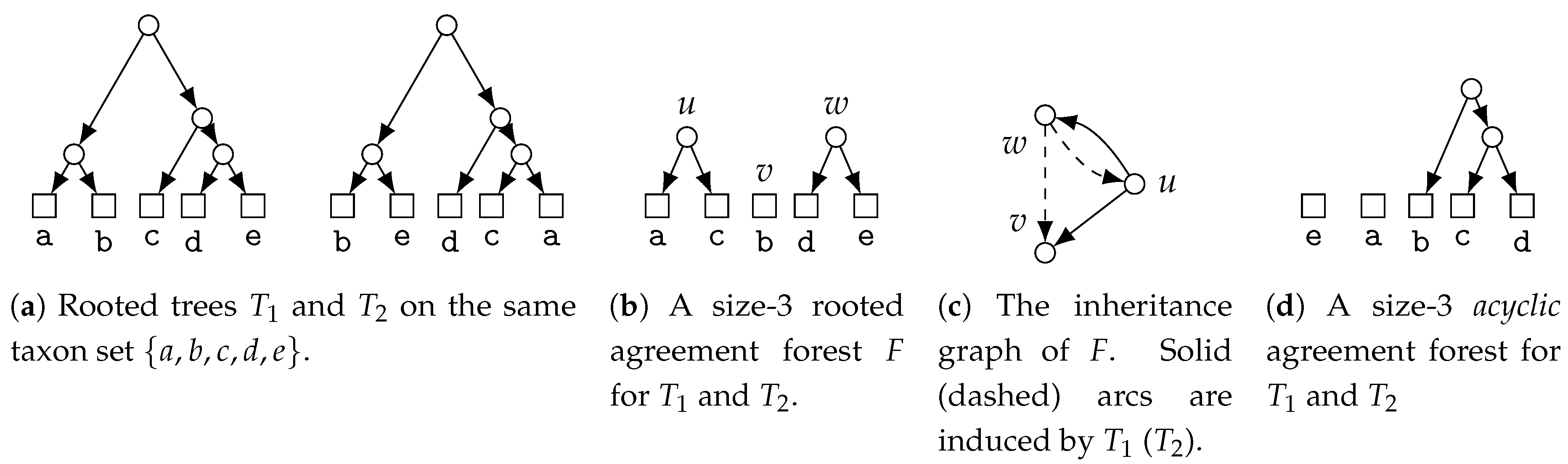
Acyclic Agreement Forest. 

The size of a MAAF of two rooted binary trees $T_1$ and $T_2$ is exactly one more than the minimum number of reticulations found in any phylogenetic network displaying both $T_1$ and $T_2$ [192] and this relation holds also if $T_1$ and $T_2$ are non-binary [203].

Deciding this number is known as the Hybridization Number (HN) problem and it has been shown to be NP-hard by Bordewich and Semple [204]. The problem can be solved in $O\left(3^{n}n\right)$ time by crawling a bounded search-tree [205]. In 2009, Whidden and Zeh claimed an $O(3^{k}nlogn)$-time algorithm, which they later retracted and replaced by an $O\left({3.18}^{k}n\right)$-time algorithm [183,195]. For $t=3$ binary trees, HN can be decided in $O^{*}\left(c^k\right)$ time, where c is an “astronomical constant” [206].

Concerning preprocessing, a kernel with at most $9k$ taxa is known [188,201] and this kernelization result has been generalized to the case of deciding HN for $t>2$ binary trees (in which case HN and MAAF no longer coincide) by van Iersel and Linz [207], showing a kernel with $20k^2$ taxa for this case, which has again been generalized to $t>2$ non-binary trees by van Iersel et al. [208], showing a kernel with at most $20k^2(\Delta -1)$ (and at most $4k{\left(5k\right)}^t$) taxa [208]. For MAAF with $t=2$ non-binary trees, Linz and Semple [203] showed a linear bikernel (that is, a kernelization into a different problem, see [209]) with $89k$ taxa, which implies a quadratic-size classical kernel. For this setting, algorithms running in $O^{*}(6^{k}k!)$ [210] and $O^{*}\left({4.83}^k\right)$ [211] time are also known.

Notes. Any algorithm for binary uMAF, rMAF, and MAAF with running time $f\left(k\right)n^{O\left(1\right)}$ can be turned into an algorithm running in $f(\ell )n^{O\left(1\right)}$, where ℓ is the level of any binary network displaying the two input trees [212]. Furthermore, all three agreement forest variants are fixed-parameter tractable for the treewidth of the display graph of the input trees [213] (see corresponding results for unrooted Tree Consistency [149,150]). The rSPR distance has been generalized to a distance measure for phylogenetic networks called SNPR and its computation is fixed-parameter tractable [214] parameterized by the distance. Variations of the discussed distance measures include: (1) the uSPR distance, which does not have an agreement-forest formulation, is NP-hard to decide [215], admits a kernel with $76k^2$ taxa [216] (in a preprint, Whidden and Matsen [217] claimed an improvement to $28k$ taxa), and can be calculated in $O^{*}(\left(28k\right)!!{16}^k)$ time [218] (using the mentioned preprint-kernel); (2) its close sibling, the replug distance, which admits a formulation as “maximum endpoint agreement forest”, is conjectured to be NP-hard to decide but admits an $O^{*}\left({16}^k\right)$-time algorithm [218]; (3) the “temporal hybridization number”, denoting the smallest amount of reticulation required to explain trees with a temporal network, which was shown to be NP-hard for two trees [219] but admits an $O^{*}\left({\left(9k\right)}^{9k}\right)$-time algorithm [220]; and (4) the parsimony distance, which is NP-hard [221,222] but can be solved in $O^{*}\left({1.618}^{38d_{\mathrm{TBR}}}\right)$ time [223], where $d_{\mathrm{TBR}}$ is the TBR distance between the input trees.

Open Questions. Consensus methods in phylogenetics can profit from a wide range of parameters, describing the particularities of likely set of inputs. While we would indeed expect that the consensus has a small distance to the input trees, a lot depends on how we choose to measure this distance. More general distance measures make for stronger parameters and, while the Hybridization Number problem can be solved in single-exponential time for the “standard parameter” k, it would be interesting to parameterize by a stronger parameter, such as the rSPR radius in which the input trees lie.

Inspired by the groundbreaking results of Bryant and Lagergren [149], research into the display graph and its treewidth has been conducted with some success [150,224]. However, we have yet to design concrete, practical algorithms for consensus problems parameterized by the treewidth of the display graph. As this would potentially yield very fast, practical algorithms, we suspect that this would be a fruitful topic in the coming years. Another interesting parameter is the “book thickness” of the display graph, that is, the minimum number of edge-colors needed to color the display graph such that each color class permits an outerplanar drawing. For obvious reasons, this parameter is smaller than the number t of input trees. Can the results for t be strengthened to work with the book thickness instead?

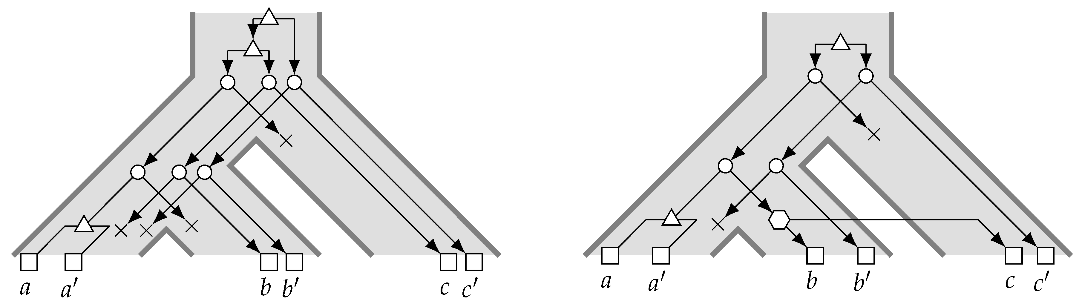
5.3. Reconciliation

Problem Description. In practice, trees depicting the evolutionary history of families of genes sampled from a set of species do not agree with the evolutionary history of the species themselves; hybridization, horizontal gene transfer, and incomplete lineage sorting being only few known causes for such discrepancies. In theory, even gene duplication and gene loss are enough to explain gene trees differing arbitrarily from the corresponding species tree. To better understand how a family of genes developed in the genome of a concurrently developing set of species, we can compute an “embedding” of the gene tree nodes to the edges of the species phylogeny called a reconciliation (see Figure 10). Reconciliations also allow drawing conclusions when comparing phylogenies of co-evolving species such as hosts/parasites or flowers/pollinators. More formally, a DL-reconciliation of a (gene-)phylogeny G with a (species-)phylogeny S is a pair $(G^{\prime },r)$ where $G^{\prime }$ is a subdivision of G and $r:V\left(G\right)\to V\left(S\right)$ is a mapping such that:

(a)

for all arcs $uv$ of G, either $r\left(u\right)=r\left(v\right)$ (in which case u is called “duplication”) or $r\left(v\right)$ is a child of $r\left(u\right)$ (in which case u is called “speciation”);

(b)

for arcs $uv$ and $uw$ in G, we have $r\left(u\right)=r\left(v\right)\iff r\left(u\right)=r\left(w\right)$ (that is, no node of G can be a speciation and a duplication at the same time); and

(c)

if u is a leaf in G, then $r\left(u\right)$ is a leaf labeled with the contemporary species that $r\left(u\right)$ was sampled in.

We can then define the number of losses in $(G^{\prime },r)$ as the sum over all speciations u of the outdegree of $r\left(u\right)$ in S minus the outdegree of u in $G^{\prime }$. If horizontal transfers are allowed, Condition (a) is replaced by

(a’)

for all arcs $uv$ of G, either $r\left(u\right)=r\left(v\right)$ (in which case u is called “duplication”) or $r\left(v\right)$ is a child of $r\left(u\right)$ (in which case u is called “speciation”), or $r\left(v\right)$ is incomparable to $r\left(u\right)$ (in which case u is called a “transfer” and $uv$ is called a “transfer arc”),

and Condition (b) is restricted to non-transfer arcs, and each transfer with out-degree one causes an additional loss. In this case, we call r a DTL-reconciliation. Since, in reality, transfers occur only between species existing at the same time, Condition (a’) introduces further restrictions. In particular, a reconciliation r is called time-consistent if G can be “dated”, that is, there is a mapping $t:V\left(G\right)\to \mathbb{N}$ such that, for all arcs $uv$ of G, we have 1. $t\left(u\right)\le t\left(v\right)$; and 2. $t\left(u\right)=t\left(v\right)$ if and only if $uv$ is a transfer arc of G under r.

A DTL-reconciliation may be time-inconsistent if, for example, there are transfer arcs $uv$ and $xy$ such that u and x are ancestors of y and v, respectively, in G.

Now, the parsimonious principle is used to define an optimization criterion. To this end, each evolutionary event is given a cost such as to reflect how unlikely it is to see a certain event. By the biological setup, it is usually assumed that speciations have cost zero.

We specify the allowed type of embedding by prepending “DL”, “DTL”, etc. to the problem name. The study of the formal reconciliation problem was initiated by Ma et al. [225] and Bonizzoni et al. [226] and is surveyed in [227,228,229,230].

Results. Optimal binary DL-reconciliations can be computed—independently of the costs—by the LCA-mapping, which maps each node of G to the LCA of the nodes that its children are mapped to [231]. Thus, this problem can be solved in linear time [232,233] using $O\left(1\right)$-time LCA queries [234,235]. The non-binary variant, while not quite as straightforward, can still be solved in polynomial time [236,237].

The complexity of computing DTL-reconciliations depends heavily on their time-consistency. If we allow producing time-inconsistent reconciliations or the given species tree already comes with a dating function, then optimal DTL-reconciliations can be computed in polynomial time [238,239,240]. In general, however, the problem is NP-hard [238,241], but can be solved in $O\left(3^k\right|G|+|S\left|\right)$ time [238]. Hallett and Lagergren [242] showed that DTL-reconciliations with at most $\alpha$ speciations mapped to any one node in the species tree is FPT in $\alpha +\tau$.

Duplication, transfer, and loss are not the only evolutionary events shaping a gene tree. Hasić and Tannier [243,244] recently introduced “replacing transfers” (T_R) and “gene conversion” (C) which model important evolutionary events and showed that DLC-reconciliations can be decided in polynomial time [243] while deciding T_R-reconciliations is NP-hard and FPT for k [244]. Finally, the concept of “incomplete lineage sorting” (ILS) is an important factor influencing discrepancies between gene and species phylogenies, especially when speciation occurs in rapid succession [245]. Roughly, ILS refers to the possibility that an earlier duplication or transfer does not pervade a population at the time a speciation occurs. Thus, one branch of a speciation may carry a gene lineage while the other does not (see Figure 11 for an illustration). In DL-reconciliation, this scenario requires a loss, but this would not reflect the true evolutionary history. Unfortunately, no particular mathematical model of ILS is widely accepted, so the following results might be incomparable. In 2017, Bork et al. [246] showed that incorporating ILS into DL-reconciliation makes the problem NP-hard, even for dated species trees. Furthermore, DTL-reconciliation for dated, non-binary species trees allows ILS to be computed in $O^{*}\left(4^{\Delta }\right)$ time [247,248].

To and Scornavacca [249] started looking into the problem of reconciling rooted gene trees with a rooted species network, showing that, for the DL model, this problem is NP-hard, but solvable in $O^{*}\left(2^k\right)$ time.

Open Questions. There are three major challenges for bioinformatics concerning reconciliation. The first and more obvious task is to include all known genomic players in the reconciliation game, meaning to establish a standard model incorporating duplication, transfer, loss, replacing transfers, conversion, and incomplete lineage sorting. While Hasić and Tannier [243,244] made good progress towards this goal, their model seems too clunky and lacks ILS support. The second challenge is to remove the need to provide $\delta$, $\tau$, etc. in the input for the Reconciliation problem. In practice, some biologists using implementations of algorithms for reconciliations just “play around” with these numbers until the results roughly fit their expectations, which is understandable since nobody knows the correct values. Indeed, in all likelihood, there are no “correct values” because the underlying assumption that the rates of genetic modification is constant throughout a phylogeny is invalid [250]. A more realistic approach might define expected frequencies of events for each branch and combine them with the length of this branch in order to dynamically price duplication, transfer, loss, etc. in this branch.

5.4. Miscellaneous

Given a phylogeny T, the parsimony score of T with respect to a labeling c of its nodes is the number of arcs in T whose extremities have a different label under c. In the Small Parsimony problem, we are given a phylogeny T and a leaf-labeling $c_L$ and have to extend $c_L$ to a labeling of all nodes of T such as to minimize the parsimony score. If T is a network, aside from the above definition (“hardwired”), the “softwired” version exists, asking for the minimum parsimony score of any tree $T^{*}$ (on the same leaf-set as T) displayed by T. While Small Parsimony is polynomial for trees [251], the problem is NP-hard in the softwired case, even for binary T and $c_L$, as well as in the hardwired case, unless $c_L$ is binary [252,253]. Fischer et al. [253] also showed that hardwired Small Parsimony is FPT for the solution parsimony score and softwired Small Parsimony is FPT for the level of the input network.

The problem of deciding whether a phylogeny T is displayed by another phylogeny N is called Tree Containment and it is NP-hard, even if T is a tree [254]. Tree Containment has polynomial-time algorithms for many special cases of N [254,255,256,257,258,259,260,261] and can be solved in $O^{*}\left({1.62}^{\ell }\right)$ time [262] (where ℓ denotes the level of N; the authors also showed an algorithm for the related Cluster Containment problem) and in $O^{*}\left(3^t\right)$ time [261], where t is the number of “invisible tree components” (that is, the number of tree-nodes u whose parent v is a reticulation that is not ”visible“ in N (that is, for each leaf a, there is a root-a-path avoiding v)). Tree Containment stays NP-hard even if the arcs of both T and N are annotated with “branch lengths”, but admits an $O^{*}\left(2^{\ell }\right)$-time algorithm in this case [263].

Recent research into the problem of rooting an unrooted network was conducted by Huber et al. [264], showing that orienting an undirected binary network as a directed network of a certain class is FPT for the level ℓ for some classes of N.

References

- Downey, R.G.; Fellows, M.R. Fundamentals of Parameterized Complexity; Texts in Computer Science; Springer: Berlin, Germany, 2013. [Google Scholar] [CrossRef]
- Cygan, M.; Fomin, F.V.; Kowalik, L.; Lokshtanov, D.; Marx, D.; Pilipczuk, M.; Pilipczuk, M.; Saurabh, S. Parameterized Algorithms; Springer: Berlin, Germany, 2015. [Google Scholar] [CrossRef]
- Ávila, L.F.; García, A.; Serna, M.J.; Thilikos, D.M. Parameterized Problems in Bioinformatics. unpublished manuscript.
- Cai, L.; Huang, X.; Liu, C.; Rosamond, F.; Song, Y. Parameterized Complexity and Biopolymer Sequence Comparison. Comput. J. 2008, 51, 270–291. [Google Scholar] [CrossRef]
- Hüffner, F.; Komusiewicz, C.; Niedermeier, R.; Wernicke, S. Parameterized Algorithmics for Finding Exact Solutions of NP-Hard Biological Problems. In Bioinformatics: Volume II: Structure, Function, and Applications; Springer: New York, NY, USA, 2017; pp. 363–402. [Google Scholar] [CrossRef]
- Gramm, J.; Nickelsen, A.; Tantau, T. Fixed-Parameter Algorithms in Phylogenetics. Comput. J. 2007, 51, 79–101. [Google Scholar] [CrossRef]
- Griffiths, A.J.; Gelbart, W.M.; Miller, J.H.; Lewontin, R.C. Chromosomal Rearrangements. In Modern Genetic Analysis; W.H.Freeman: New York, NY, USA, 1999; Chapter 8. [Google Scholar]
- Fertin, G.; Labarre, A.; Rusu, I.; Tannier, E.; Vialette, S. Combinatorics of Genome Rearrangements; Computational Molecular Biology; MIT Press: Cambridge, MA, USA, 2009; p. 312. [Google Scholar]
- Yancopoulos, S.; Attie, O.; Friedberg, R. Efficient sorting of genomic permutations by translocation, inversion and block interchange. Bioinformatics 2005, 21, 3340–3346. [Google Scholar] [CrossRef]
- Bergeron, A.; Mixtacki, J.; Stoye, J. A unifying view of genome rearrangements. In International Workshop on Algorithms in Bioinformatics; Springer: Berlin, Germany, 2006; pp. 163–173. [Google Scholar]
- Chauve, C.; Fertin, G.; Rizzi, R.; Vialette, S. Genomes containing duplicates are hard to compare. In International Conference on Computational Science; Springer: Berlin, Germany, 2006; pp. 783–790. [Google Scholar]
- Jiang, H.; Zhu, B.; Zhu, D. Algorithms for sorting unsigned linear genomes by the DCJ operations. Bioinformatics 2010, 27, 311–316. [Google Scholar] [CrossRef]
- Fertin, G.; Jean, G.; Tannier, E. Algorithms for computing the double cut and join distance on both gene order and intergenic sizes. Algorithms Mol. Biol. 2017, 12, 16. [Google Scholar] [CrossRef]
- Bérard, S.; Chateau, A.; Chauve, C.; Paul, C.; Tannier, E. Perfect DCJ rearrangement. In RECOMB International Workshop on Comparative Genomics; Springer: Berlin, Germany, 2008; pp. 158–169. [Google Scholar]
- Watterson, G.; Ewens, W.; Hall, T.; Morgan, A. The chromosome inversion problem. J. Theor. Biol. 1982, 99, 1–7. [Google Scholar] [CrossRef]
- Hannenhalli, S.; Pevzner, P.A. Transforming Cabbage into Turnip: Polynomial Algorithm for Sorting Signed Permutations by Reversals. J. ACM 1999, 46, 1–27. [Google Scholar] [CrossRef]
- Christie, D.A. Genome Rearrangement Problems. Ph.D. Thesis, University of Glasgow, Glasgow, UK, 1998. [Google Scholar]
- Chen, X.; Zheng, J.; Fu, Z.; Nan, P.; Zhong, Y.; Lonardi, S.; Jiang, T. Assignment of Orthologous Genes via Genome Rearrangement. IEEE/ACM Trans. Comput. Biol. Bioinform. 2005, 2, 302–315. [Google Scholar] [CrossRef]
- Radcliffe, A.; Scott, A.; Wilmer, E. Reversals and transpositions over finite alphabets. SIAM J. Discret. Math. 2006, 19, 224. [Google Scholar] [CrossRef]
- Kececioglu, J.; Sankoff, D. Exact and approximation algorithms for sorting by reversals, with application to genome rearrangement. Algorithmica 1995, 13, 180. [Google Scholar] [CrossRef]
- Bulteau, L.; Fertin, G.; Komusiewicz, C. Reversal distances for strings with few blocks or small alphabets. In Symposium on Combinatorial Pattern Matching; Springer: Berlin, Germany, 2014; pp. 50–59. [Google Scholar]
- Bérard, S.; Chauve, C.; Paul, C. A more efficient algorithm for perfect sorting by reversals. Inf. Process. Lett. 2008, 106, 90–95. [Google Scholar] [CrossRef]
- Dias, Z.; Meidanis, J. Sorting by prefix transpositions. In International Symposium on String Processing and Information Retrieval; Springer: Berlin, Germany, 2002; pp. 65–76. [Google Scholar]
- Whidden, C. Sorting by Transpositions: Fixed-Parameter Algorithms and Structural Properties. Bachelor’s Thesis, Dalhousie University, Halifax, NS, Canada, 2007. [Google Scholar]
- Fertin, G.; Jankowiak, L.; Jean, G. Prefix and suffix reversals on strings. Discret. Appl. Math. 2018, 246, 140–153. [Google Scholar] [CrossRef]
- Lopresti, D.; Tomkins, A. Block edit models for approximate string matching. Theor. Comput. Sci. 1997, 181, 159–179. [Google Scholar] [CrossRef]
- Swenson, K.M.; Marron, M.; Earnest-DeYoung, J.V.; Moret, B.M. Approximating the true evolutionary distance between two genomes. J. Exp. Algorithmics (JEA) 2008, 12, 3–5. [Google Scholar] [CrossRef]
- Damaschke, P. Minimum common string partition parameterized. In International Workshop on Algorithms in Bioinformatics; Springer: Berlin, Germany, 2008; pp. 87–98. [Google Scholar]
- Jiang, H.; Zhu, B.; Zhu, D.; Zhu, H. Minimum common string partition revisited. J. Comb. Optim. 2012, 23, 519–527. [Google Scholar] [CrossRef]
- Bulteau, L.; Komusiewicz, C. Minimum common string partition parameterized by partition size is fixed-parameter tractable. In Proceedings of the Twenty-Fifth Annual ACM-SIAM Symposium on Discrete Algorithms, SIAM, Portland, OR, USA, 5–7 January 2014; pp. 102–121. [Google Scholar]
- Bulteau, L.; Fertin, G.; Komusiewicz, C.; Rusu, I. A fixed-parameter algorithm for minimum common string partition with few duplications. In International Workshop on Algorithms in Bioinformatics; Springer: Berlin, Germany, 2013; pp. 244–258. [Google Scholar]
- Beretta, S.; Castelli, M.; Dondi, R. Parameterized tractability of the maximum-duo preservation string mapping problem. Theor. Comput. Sci. 2016, 646, 16–25. [Google Scholar] [CrossRef][Green Version]
- Zheng, C.; Zhu, Q.; Sankoff, D. Removing noise and ambiguities from comparative maps in rearrangement analysis. IEEE/ACM Trans. Comput. Biol. Bioinform. 2007, 4, 515–522. [Google Scholar] [CrossRef] [PubMed]
- Li, W.; Liu, H.; Wang, J.; Xiang, L.; Yang, Y. An improved linear kernel for complementary maximal strip recovery: Simpler and smaller. Theor. Comput. Sci. 2019, 786, 55–66. [Google Scholar] [CrossRef]
- Bulteau, L.; Fertin, G.; Jiang, M.; Rusu, I. Tractability and approximability of maximal strip recovery. Theor. Comput. Sci. 2012, 440, 14–28. [Google Scholar] [CrossRef]
- Jiang, M. On the parameterized complexity of some optimization problems related to multiple-interval graphs. Theor. Comput. Sci. 2010, 411, 4253–4262. [Google Scholar] [CrossRef]
- Muñoz, A.; Zheng, C.; Zhu, Q.; Albert, V.A.; Rounsley, S.; Sankoff, D. Scaffold filling, contig fusion and comparative gene order inference. BMC Bioinform. 2010, 11, 304. [Google Scholar] [CrossRef] [PubMed]
- Bulteau, L.; Carrieri, A.P.; Dondi, R. Fixed-parameter algorithms for scaffold filling. Theor. Comput. Sci. 2015, 568, 72–83. [Google Scholar] [CrossRef]
- Sankoff, D.; Blanchette, M. Multiple genome rearrangement and breakpoint phylogeny. J. Comput. Biol. 1998, 5, 555–570. [Google Scholar] [CrossRef] [PubMed]
- Waterston, R.H.; Lander, E.S.; Sulston, J.E. On the sequencing of the human genome. Proc. Natl. Acad. Sci. USA 2002, 99, 3712–3716. [Google Scholar] [CrossRef]
- Notredame, C. Recent Evolutions of Multiple Sequence Alignment Algorithms. PLOS Comput. Biol. 2007, 3, 1–4. [Google Scholar] [CrossRef]
- Bonizzoni, P.; Della Vedova, G. The complexity of multiple sequence alignment with SP-score that is a metric. Theor. Comput. Sci. 2001, 259, 63–79. [Google Scholar] [CrossRef]
- Just, W. Computational complexity of multiple sequence alignment with SP-score. J. Comput. Biol. 2001, 8, 615–623. [Google Scholar] [CrossRef]
- Elias, I. Settling the intractability of multiple alignment. In International Symposium on Algorithms and Computation; Springer: Berlin, Germany, 2003; pp. 352–363. [Google Scholar]
- Kemena, C.; Notredame, C. Upcoming challenges for multiple sequence alignment methods in the high-throughput era. Bioinformatics 2009, 25, 2455–2465. [Google Scholar] [CrossRef]
- Bulteau, L.; Hüffner, F.; Komusiewicz, C.; Niedermeier, R. Multivariate Algorithmics for NP-Hard String Problems. Bull. EATCS 2014, 114, 1–43. [Google Scholar]
- Frances, M.; Litman, A. On covering problems of codes. Theory Comput. Syst. 1997, 30, 113–119. [Google Scholar] [CrossRef]
- Gramm, J.; Niedermeier, R.; Rossmanith, P. Fixed-parameter algorithms for closest string and related problems. Algorithmica 2003, 37, 25–42. [Google Scholar] [CrossRef]
- Evans, P.A.; Smith, A.D.; Wareham, H.T. On the complexity of finding common approximate substrings. Theor. Comput. Sci. 2003, 306, 407–430. [Google Scholar] [CrossRef]
- Fellows, M.R.; Gramm, J.; Niedermeier, R. On the parameterized intractability of motif search problems. Combinatorica 2006, 26, 141–167. [Google Scholar] [CrossRef]
- Marx, D. Closest substring problems with small distances. SIAM J. Comput. 2008, 38, 1382–1410. [Google Scholar] [CrossRef][Green Version]
- Schmid, M.L. Finding consensus strings with small length difference between input and solution strings. ACM Trans. Comput. Theory (TOCT) 2017, 9, 13. [Google Scholar] [CrossRef]
- Boucher, C.; Ma, B. Closest string with outliers. BMC Bioinform. 2011, 12, S55. [Google Scholar] [CrossRef]
- Bulteau, L.; Schmid, M. Consensus Strings with Small Maximum Distance and Small Distance Sum. In Proceedings of the 43rd International Symposium on Mathematical Foundations of Computer Science (MFCS 2018), Liverpool, UK, 27–31 August 2018. [Google Scholar]
- Chen, J.; Hermelin, D.; Sorge, M. On Computing Centroids According to the p-Norms of Hamming Distance Vectors. In Proceedings of the 27th Annual European Symposium on Algorithms, ESA 2019, Schloss Dagstuhl—Leibniz-Zentrum für Informatik, Munich/Garching, Germany, 9–11 September 2019; Volume 144, pp. 28:1–28:16. [Google Scholar] [CrossRef]
- Pietrzak, K. On the parameterized complexity of the fixed alphabet shortest common supersequence and longest common subsequence problems. J. Comput. Syst. Sci. 2003, 67, 757–771. [Google Scholar] [CrossRef]
- Bodlaender, H.L.; Downey, R.G.; Fellows, M.R.; Wareham, H.T. The parameterized complexity of sequence alignment and consensus. Theor. Comput. Sci. 1995, 147, 31–54. [Google Scholar] [CrossRef]
- Irving, R.W.; Fraser, C.B. Two algorithms for the longest common subsequence of three (or more) strings. In Annual Symposium on Combinatorial Pattern Matching; Springer: Berlin, Germany, 1992; pp. 214–229. [Google Scholar]
- Abboud, A.; Backurs, A.; Williams, V.V. Tight hardness results for LCS and other sequence similarity measures. In Proceedings of the 2015 IEEE 56th Annual Symposium on Foundations of Computer Science, Berkeley, CA, USA, 17–20 October 2015; pp. 59–78. [Google Scholar]
- Bringmann, K.; Künnemann, M. Multivariate fine-grained complexity of longest common subsequence. In Proceedings of the Twenty-Ninth Annual ACM-SIAM Symposium on Discrete Algorithms, Society for Industrial and Applied Mathematics, New Orleans, LA, USA, 7–10 January 2018; pp. 1216–1235. [Google Scholar]
- Giannopoulou, A.C.; Mertzios, G.B.; Niedermeier, R. Polynomial fixed-parameter algorithms: A case study for longest path on interval graphs. Theor. Comput. Sci. 2017, 689, 67–95. [Google Scholar] [CrossRef]
- Mertzios, G.B.; Nichterlein, A.; Niedermeier, R. The Power of Linear-Time Data Reduction for Maximum Matching. In Proceedings of the 42nd International Symposium on Mathematical Foundations of Computer Science (MFCS 2017), Aalborg, Denmark, 21–25 August 2017; Schloss Dagstuhl–Leibniz-Zentrum fuer Informatik: Dagstuhl, Germany, 2017; Volume 83, pp. 46:1–46:14. [Google Scholar] [CrossRef]
- Coudert, D.; Ducoffe, G.; Popa, A. Fully Polynomial FPT Algorithms for Some Classes of Bounded Clique-width Graphs. ACM Trans. Algorithms 2019, 15, 33:1–33:57. [Google Scholar] [CrossRef]
- Tsai, Y.T. The constrained longest common subsequence problem. Inf. Process. Lett. 2003, 88, 173–176. [Google Scholar] [CrossRef]
- Bonizzoni, P.; Della Vedova, G.; Dondi, R.; Pirola, Y. Variants of constrained longest common subsequence. Inf. Process. Lett. 2010, 110, 877–881. [Google Scholar] [CrossRef]
- Chen, Y.C.; Chao, K.M. On the generalized constrained longest common subsequence problems. J. Comb. Optim. 2011, 21, 383–392. [Google Scholar] [CrossRef]
- Gotthilf, Z.; Hermelin, D.; Landau, G.M.; Lewenstein, M. Restricted lcs. In International Symposium on String Processing and Information Retrieval; Springer: Berlin, Germany, 2010; pp. 250–257. [Google Scholar]
- Chen, J.; Huang, X.; Kanj, I.A.; Xia, G. On the computational hardness based on linear FPT-reductions. J. Comb. Optim. 2006, 11, 231–247. [Google Scholar] [CrossRef]
- Fellows, M.; Hallett, M.; Korostensky, C.; Stege, U. Analogs and Duals of the MAST Problem for Sequences and Trees. In European Symposium on Algorithms; Springer: Berlin, Germany, 1998; pp. 103–114. [Google Scholar]
- Nicolas, F.; Rivals, E. Complexities of the centre and median string problems. In Annual Symposium on Combinatorial Pattern Matching; Springer: Berlin, Germany, 2003; pp. 315–327. [Google Scholar]
- Maji, H.; Izumi, T. Listing center strings under the edit distance metric. In Combinatorial Optimization and Applications; Springer: Berlin, Germany, 2015; pp. 771–782. [Google Scholar]
- Hunt, M.; Newbold, C.; Berriman, M.; Otto, T.D. A comprehensive evaluation of assembly scaffolding tools. Genome Biol. 2014, 15, R42. [Google Scholar] [CrossRef] [PubMed]
- Huson, D.H.; Reinert, K.; Myers, E.W. The Greedy Path-merging Algorithm for Contig Scaffolding. J. ACM 2002, 49, 603–615. [Google Scholar] [CrossRef]
- Chateau, A.; Giroudeau, R.; Poss, M.; Weller, M. Scaffolding with repeated contigs using flow formulations. unpublished manuscript.
- Weller, M.; Chateau, A.; Dallard, C.; Giroudeau, R. Scaffolding Problems Revisited: Complexity, Approximation and Fixed Parameter Tractable Algorithms, and Some Special Cases. Algorithmica 2018, 80, 1771–1803. [Google Scholar] [CrossRef]
- Gao, S.; Sung, W.K.; Nagarajan, N. Opera: Reconstructing Optimal Genomic Scaffolds with High-Throughput Paired-End Sequences. J. Comput. Biol. 2011, 18, 1681–1691. [Google Scholar] [CrossRef]
- Weller, M.; Chateau, A.; Giroudeau, R. Exact approaches for scaffolding. BMC Bioinform. 2015, 16, S2. [Google Scholar] [CrossRef]
- Weller, M.; Chateau, A.; Giroudeau, R. On the Linearization of Scaffolds Sharing Repeated Contigs. In Proceedings of the 11th International Conference on Combinatorial Optimization and Applications (COCOA’17) Part II, Shanghai, China, 16–18 December 2017; pp. 509–517. [Google Scholar] [CrossRef]
- Davot, T.; Chateau, A.; Giroudeau, R.; Weller, M. Linearizing Genomes: Exact Methods and Local Search. In Proceedings of the SOFSEM’20, Nový Smokovec, Slovakia, 27–30 January 2019. [Google Scholar]
- Donmez, N.; Brudno, M. SCARPA: scaffolding reads with practical algorithms. Bioinformatics 2012, 29, 428–434. [Google Scholar] [CrossRef]
- Cao, M.D.; Nguyen, S.H.; Ganesamoorthy, D.; Elliott, A.G.; Cooper, M.A.; Coin, L.J.M. Scaffolding and completing genome assemblies in real-time with nanopore sequencing. Nat. Commun. 2017, 8, 14515. [Google Scholar] [CrossRef]
- Dallard, C.; Weller, M.; Chateau, A.; Giroudeau, R. Instance Guaranteed Ratio on Greedy Heuristic for Genome Scaffolding. In Combinatorial Optimization and Applications; Springer International Publishing: Cham, Switzerland, 2016; pp. 294–308. [Google Scholar]
- Hodgkinson, A.; Eyre-Walker, A. Human triallelic sites: Evidence for a new mutational mechanism? Genetics 2010, 184, 233–241. [Google Scholar] [CrossRef][Green Version]
- International SNP Map Working Group. A map of human genome sequence variation containing 1.42 million single nucleotide polymorphisms. Nature 2001, 409, 928. [Google Scholar] [CrossRef]
- Andrés, A.M.; Clark, A.G.; Shimmin, L.; Boerwinkle, E.; Sing, C.F.; Hixson, J.E. Understanding the accuracy of statistical haplotype inference with sequence data of known phase. Genet. Epidemiol. 2007, 31, 659–671. [Google Scholar] [CrossRef] [PubMed]
- Orzack, S.H.; Gusfield, D.; Olson, J.; Nesbitt, S.; Subrahmanyan, L.; Stanton, V.P. Analysis and Exploration of the Use of Rule-Based Algorithms and Consensus Methods for the Inferral of Haplotypes. Genetics 2003, 165, 915–928. [Google Scholar]
- Climer, S.; Jäger, G.; Templeton, A.R.; Zhang, W. How frugal is mother nature with haplotypes? Bioinformatics 2008, 25, 68–74. [Google Scholar] [CrossRef]
- Zhang, X.S.; Wang, R.S.; Wu, L.Y.; Chen, L. Models and Algorithms for Haplotyping Problem. Curr. Bioinform. 2006, 1, 105–114. [Google Scholar] [CrossRef]
- Halldórsson, B.V.; Bafna, V.; Edwards, N.; Lippert, R.; Yooseph, S.; Istrail, S. A Survey of Computational Methods for Determining Haplotypes. In Computational Methods for SNPs and Haplotype Inference; Springer: Berlin/Heidelberg, Germany, 2004; pp. 26–47. [Google Scholar]
- Lancia, G. Algorithmic approaches for the single individual haplotyping problem. RAIRO Recherche Opérationnelle 2016, 50. [Google Scholar] [CrossRef]
- Zhao, Y.; Xu, Y.; Zhang, Q.; Chen, G. An overview of the haplotype problems and algorithms. Front. Comput. Sci. China 2007, 1, 272–282. [Google Scholar] [CrossRef]
- Schwartz, R. Theory and Algorithms for the Haplotype Assembly Problem. Commun. Inf. Syst. 2010, 10, 23–38. [Google Scholar] [CrossRef]
- Geraci, F. A comparison of several algorithms for the single individual SNP haplotyping reconstruction problem. Bioinformatics 2010, 26, 2217–2225. [Google Scholar] [CrossRef]
- Xie, M.; Wang, J.; Chen, J.; Wu, J.; Liu, X. Computational Models and Algorithms for the Single Individual Haplotyping Problem. Curr. Bioinform. 2010, 5, 18–28. [Google Scholar] [CrossRef]
- Rhee, J.K.; Li, H.; Joung, J.G.; Hwang, K.B.; Zhang, B.T.; Shin, S.Y. Survey of computational haplotype determination methods for single individual. Genes Genom. 2016, 38, 1–12. [Google Scholar] [CrossRef]
- Lancia, G.; Bafna, V.; Istrail, S.; Lippert, R.; Schwartz, R. SNPs Problems, Complexity, and Algorithms. In Algorithms—ESA 2001; Springer: Berlin/Heidelberg, Germany, 2001; pp. 182–193. [Google Scholar]
- Bafna, V.; Istrail, S.; Lancia, G.; Rizzi, R. Polynomial and APX-hard cases of the individual haplotyping problem. Theor. Comput. Sci. 2005, 335, 109–125. [Google Scholar] [CrossRef]
- Xie, M.; Wang, J. An Improved (and Practical) Parameterized Algorithm for the Individual Haplotyping Problem MFR with Mate-Pairs. Algorithmica 2008, 52, 250–266. [Google Scholar] [CrossRef]
- Reed, B.; Smith, K.; Vetta, A. Finding odd cycle transversals. Oper. Res. Lett. 2004, 32, 299–301. [Google Scholar] [CrossRef]
- Hüffner, F. Algorithm Engineering for Optimal Graph Bipartization. J. Graph Algorithms Appl. 2009, 13, 77–98. [Google Scholar] [CrossRef]
- Lokshtanov, D.; Narayanaswamy, N.S.; Raman, V.; Ramanujan, M.S.; Saurabh, S. Faster Parameterized Algorithms Using Linear Programming. ACM Trans. Algorithms 2014, 11, 15:1–15:31. [Google Scholar] [CrossRef]
- Kratsch, S.; Wahlström, M. Compression via Matroids: A Randomized Polynomial Kernel for Odd Cycle Transversal. ACM Trans. Algorithms 2014, 10, 20:1–20:15. [Google Scholar] [CrossRef]
- Xie, M.; Chen, J.; Wang, J. Research on parameterized algorithms of the individual haplotyping problem. J. Bioinform. Comput. Biol. 2007, 5, 795–816. [Google Scholar] [CrossRef]
- Cilibrasi, R.; van Iersel, L.; Kelk, S.; Tromp, J. The Complexity of the Single Individual SNP Haplotyping Problem. Algorithmica 2007, 49, 13–36. [Google Scholar] [CrossRef]
- Bonizzoni, P.; Dondi, R.; Klau, G.W.; Pirola, Y.; Pisanti, N.; Zaccaria, S. On the Minimum Error Correction Problem for Haplotype Assembly in Diploid and Polyploid Genomes. J. Comput. Biol. 2016, 23, 718–736. [Google Scholar] [CrossRef] [PubMed]
- Wang, R.S.; Wu, L.Y.; Li, Z.P.; Zhang, X.S. Haplotype reconstruction from SNP fragments by minimum error correction. Bioinformatics 2005, 21, 2456–2462. [Google Scholar] [CrossRef] [PubMed]
- Xie, M.; Wang, J.; Chen, J. A model of higher accuracy for the individual haplotyping problem based on weighted SNP fragments and genotype with errors. Bioinformatics 2008, 24, i105–i113. [Google Scholar] [CrossRef][Green Version]
- Deng, F.; Cui, W.; Wang, L. A highly accurate heuristic algorithm for the haplotype assembly problem. BMC Genom. 2013, 14, S2. [Google Scholar] [CrossRef] [PubMed]
- Patterson, M.; Marschall, T.; Pisanti, N.; van Iersel, L.; Stougie, L.; Klau, G.W.; Schönhuth, A. WhatsHap: Weighted Haplotype Assembly for Future-Generation Sequencing Reads. J. Comput. Biol. 2015, 22, 498–509. [Google Scholar] [CrossRef]
- Pirola, Y.; Zaccaria, S.; Dondi, R.; Klau, G.W.; Pisanti, N.; Bonizzoni, P. HapCol: accurate and memory-efficient haplotype assembly from long reads. Bioinformatics 2015, 32, 1610–1617. [Google Scholar] [CrossRef][Green Version]
- Garg, S.; Rautiainen, M.; Novak, A.M.; Garrison, E.; Durbin, R.; Marschall, T. A graph-based approach to diploid genome assembly. Bioinformatics 2018, 34, i105–i114. [Google Scholar] [CrossRef]
- He, D.; Choi, A.; Pipatsrisawat, K.; Darwiche, A.; Eskin, E. Optimal algorithms for haplotype assembly from whole-genome sequence data. Bioinformatics 2010, 26, i183–i190. [Google Scholar] [CrossRef]
- Zhang, X.S.; Wang, R.S.; Wu, L.Y.; Zhang, W. Minimum Conflict Individual Haplotyping from SNP Fragments and Related Genotype. Evolut. Bioinform. 2006, 2. [Google Scholar] [CrossRef]
- Hermelin, D.; Rozenberg, L. Parameterized complexity analysis for the Closest String with Wildcards problem. Theor. Comput. Sci. 2015, 600, 11–18. [Google Scholar] [CrossRef]
- Garg, S.; Martin, M.; Marschall, T. Read-based phasing of related individuals. Bioinformatics 2016, 32, i234–i242. [Google Scholar] [CrossRef]
- Li, Z.p.; Wu, L.y.; Zhao, Y.y.; Zhang, X.s. A Dynamic Programming Algorithm for the k-Haplotyping Problem. Acta Mathematicae Applicatae Sinica 2006, 22, 405–412. [Google Scholar] [CrossRef]
- Bao, R.; Huang, L.; Andrade, J.; Tan, W.; Kibbe, W.A.; Jiang, H.; Feng, G. Review of Current Methods, Applications, and Data Management for the Bioinformatics Analysis of Whole Exome Sequencing. Cancer Inform. 2014, 13s2, CIN.S13779. [Google Scholar] [CrossRef]
- Garg, S. Computational Haplotyping: Theory and Practice. Ph.D. Thesis, Universität des Saarlandes, Saarbrücken, Germany, 2018. [Google Scholar] [CrossRef]
- Gusfield, D. Haplotype Inference by Pure Parsimony. In Combinatorial Pattern Matching; Springer: Berlin/Heidelberg, Germany, 2003; pp. 144–155. [Google Scholar]
- Bonizzoni, P.; Della Vedova, G.; Dondi, R.; Pirola, Y.; Rizzi, R. Pure Parsimony Xor Haplotyping. IEEE/ACM Trans. Comput. Biol. Bioinform. 2010, 7, 598–610. [Google Scholar] [CrossRef] [PubMed]
- Graça, A.; Lynce, I.; Marques-Silva, J.; Oliveira, A.L. Haplotype Inference by Pure Parsimony: A Survey. J. Comput. Biol. 2010, 17, 969–992. [Google Scholar] [CrossRef]
- Hubbell, E.; (GRAIL, Inc. LinkedIn, Menlo Park, CA, USA). Finding a Parsimony Solution to Haplotype Phase is NP-Hard. Personal communication, 2002. [Google Scholar]
- Lancia, G.; Pinotti, M.C.; Rizzi, R. Haplotyping Populations by Pure Parsimony: Complexity of Exact and Approximation Algorithms. INFORMS J. Comput. 2004, 16, 348–359. [Google Scholar] [CrossRef]
- Huang, Y.T.; Chao, K.M.; Chen, T. An Approximation Algorithm for Haplotype Inference by Maximum Parsimony. J. Comput. Biol. 2005, 12, 1261–1274. [Google Scholar] [CrossRef]
- Sharan, R.; Halldorsson, B.V.; Istrail, S. Islands of Tractability for Parsimony Haplotyping. IEEE/ACM Trans. Comput. Biol. Bioinform. 2006, 3, 303–311. [Google Scholar] [CrossRef]
- van Iersel, L.; Keijsper, J.; Kelk, S.; Stougie, L. Shorelines of Islands of Tractability: Algorithms for Parsimony and Minimum Perfect Phylogeny Haplotyping Problems. IEEE/ACM Trans. Comput. Biol. Bioinform. 2008, 5, 301–312. [Google Scholar] [CrossRef]
- Lancia, G.; Rizzi, R. A polynomial case of the parsimony haplotyping problem. Oper. Res. Lett. 2006, 34, 289–295. [Google Scholar] [CrossRef]
- van Iersel, L.J.J. Algorithms, Haplotypes and Phylogenetic Networks. Ph.D. Thesis, Eindhoven University of Technology, Eindhoven, The Netherlands, 2009. [Google Scholar]
- Fellows, M.R.; Hartman, T.; Hermelin, D.; Landau, G.M.; Rosamond, F.A.; Rozenberg, L. Haplotype Inference Constrained by Plausible Haplotype Data. IEEE/ACM Trans. Comput. Biol. Bioinform. 2011, 8, 1692–1699. [Google Scholar] [CrossRef] [PubMed]
- Fleischer, R.; Guo, J.; Niedermeier, R.; Uhlmann, J.; Wang, Y.; Weller, M.; Wu, X. Extended Islands of Tractability for Parsimony Haplotyping. In Combinatorial Pattern Matching; Springer: Berlin/Heidelberg, Germany, 2010; pp. 214–226. [Google Scholar]
- Gusfield, D. Haplotyping As Perfect Phylogeny: Conceptual Framework and Efficient Solutions. In Proceedings of the Sixth Annual International Conference on Computational Biology, RECOMB ’02, Washington, DC, USA, 18–21 April 2002; ACM: New York, NY, USA, 2002; pp. 166–175. [Google Scholar] [CrossRef]
- Ding, Z.; Filkov, V.; Gusfield, D. A Linear-Time Algorithm for the Perfect Phylogeny Haplotyping (PPH) Problem. J. Comput. Biol. 2006, 13, 522–553. [Google Scholar] [CrossRef] [PubMed]
- Bonizzoni, P. A Linear-Time Algorithm for the Perfect Phylogeny Haplotype Problem. Algorithmica 2007, 48, 267–285. [Google Scholar] [CrossRef]
- Chen, Z.Z.; Ma, W.; Wang, L. The Parameterized Complexity of the Shared Center Problem. Algorithmica 2014, 69, 269–293. [Google Scholar] [CrossRef][Green Version]
- Keijsper, J.; Oosterwijk, T. Tractable Cases of (*, 2)-Bounded Parsimony Haplotyping. IEEE/ACM Trans. Comput. Biol. Bioinform. 2015, 12, 234–247. [Google Scholar] [CrossRef]
- Cicalese, F.; Milanivc, M. On Parsimony Haplotyping; Technical Report; Universitẗ Bielefeld: Bielefeld, Germany, 2008. [Google Scholar]
- Haeckel, E. Generelle Morphologie der Organismen. Allgemeine Grundzüge der organischen Formen-Wissenschaft, mechanisch begründet durch die von C. Darwin reformirte Descendenz-Theorie, etc.; Verlag von Georg Reimer: Berlin, Germany, 1866; Volume 2. [Google Scholar]
- Dobzhansky, T. Nothing in Biology Makes Sense except in the Light of Evolution. Am. Biol. Teach. 1973, 35, 125–129. [Google Scholar] [CrossRef]
- De Bruyn, A.; Martin, D.P.; Lefeuvre, P. Phylogenetic Reconstruction Methods: An Overview. In Molecular Plant Taxonomy: Methods and Protocols; Humana Press: Totowa, NJ, USA, 2014; pp. 257–277. [Google Scholar] [CrossRef]
- Huson, D.H.; Rupp, R.; Scornavacca, C. Phylogenetic Networks—Concepts, Algorithms and Applications; Cambridge University Press: Cambridge, UK, 2010. [Google Scholar]
- Choy, C.; Jansson, J.; Sadakane, K.; Sung, W.K. Computing the maximum agreement of phylogenetic networks. Theor. Comput. Sci. 2005, 335, 93–107. [Google Scholar] [CrossRef]
- Betzler, N.; Guo, J.; Komusiewicz, C.; Niedermeier, R. Average parameterization and partial kernelization for computing medians. J. Comput. Syst. Sci. 2011, 77, 774–789. [Google Scholar] [CrossRef]
- Bryant, D. A classification of consensus methods for phylogenetics. DIMACS Ser. Discrete Math. Theor. Comput. Sci. 2003, 61, 163–184. [Google Scholar]
- Degnan, J.H. Consensus Methods, Phylogenetic. In Encyclopedia of Evolutionary Biology; Elsevier: Amsterdam, The Netherlands, 2016; Volume 1, pp. 341–346. [Google Scholar]
- Steel, M. The complexity of reconstructing trees from qualitative characters and subtrees. J. Classif. 1992, 9, 91–116. [Google Scholar] [CrossRef]
- Böcker, S.; Bryant, D.; Dress, A.W.; Steel, M.A. Algorithmic Aspects of Tree Amalgamation. J. Algorithms 2000, 37, 522–537. [Google Scholar] [CrossRef]
- Arnborg, S.; Lagergren, J.; Seese, D. Easy problems for tree-decomposable graphs. J. Algorithms 1991, 12, 308–340. [Google Scholar] [CrossRef]
- Courcelle, B. The monadic second-order logic of graphs. I. Recognizable sets of finite graphs. Inf. Comput. 1990, 85, 12–75. [Google Scholar] [CrossRef]
- Bryant, D.; Lagergren, J. Compatibility of unrooted phylogenetic trees is FPT. Theor. Comput. Sci. 2006, 351, 296–302. [Google Scholar] [CrossRef]
- Scornavacca, C.; van Iersel, L.; Kelk, S.; Bryant, D. The agreement problem for unrooted phylogenetic trees is FPT. J. Graph Algorithms Appl. 2014, 18, 385–392. [Google Scholar] [CrossRef][Green Version]
- Baste, J.; Paul, C.; Sau, I.; Scornavacca, C. Efficient FPT Algorithms for (Strict) Compatibility of Unrooted Phylogenetic Trees. In Algorithmic Aspects in Information and Management; Springer International Publishing: Cham, Switzerland, 2016; pp. 53–64. [Google Scholar]
- Aho, A.; Sagiv, Y.; Szymanski, T.; Ullman, J. Inferring a Tree from Lowest Common Ancestors with an Application to the Optimization of Relational Expressions. SIAM J. Comput. 1981, 10, 405–421. [Google Scholar] [CrossRef]
- Ng, M.P.; Wormald, N.C. Reconstruction of rooted trees from subtrees. Discret. Appl. Math. 1996, 69, 19–31. [Google Scholar] [CrossRef]
- Maddison, W.P. Gene Trees in Species Trees. Syst. Biol. 1997, 46, 523–536. [Google Scholar] [CrossRef]
- Linder, C.R.; Rieseberg, L.H. Reconstructing patterns of reticulate evolution in plants. Am. J. Bot. 2004, 91, 1700–1708. [Google Scholar] [CrossRef]
- Jansson, J. On the complexity of inferring rooted evolutionary trees. Electron. Notes Discret. Math. 2001, 7, 50–53. [Google Scholar] [CrossRef]
- Bryant, D. Building Trees, Hunting for Trees, and Comparing Trees: Theory and Methods in Phylogenetic Analysis. Ph.D. Thesis, University of Canterbury, Canterbury, UK, 1997. [Google Scholar]
- Wu, B.Y. Constructing the Maximum Consensus Tree from Rooted Triples. J. Comb. Optim. 2004, 8, 29–39. [Google Scholar] [CrossRef]
- Byrka, J.; Guillemot, S.; Jansson, J. New results on optimizing rooted triplets consistency. Discret. Appl. Math. 2010, 158, 1136–1147. [Google Scholar] [CrossRef]
- Guillemot, S.; Mnich, M. Kernel and Fast Algorithm for Dense Triplet Inconsistency. In Theory and Applications of Models of Computation; Springer: Berlin/Heidelberg, Germany, 2010; pp. 247–257. [Google Scholar]
- Fomin, F.V.; Lokshtanov, D.; Saurabh, S.; Zehavi, M. Kernelization: Theory of Parameterized Preprocessing; Cambridge University Press: Cambridge, UK, 2019. [Google Scholar] [CrossRef]
- Paul, C.; Perez, A.; Thomassé, S. Linear kernel for Rooted Triplet Inconsistency and other problems based on conflict packing technique. J. Comput. Syst. Sci. 2016, 82, 366–379. [Google Scholar] [CrossRef]
- Habib, M.; To, T.H. Constructing a minimum phylogenetic network from a dense triplet set. J. Bioinform. Comput. Biol. 2012, 10, 1250013. [Google Scholar] [CrossRef] [PubMed]
- van Iersel, L.; Kelk, S. Constructing the Simplest Possible Phylogenetic Network from Triplets. Algorithmica 2011, 60, 207–235. [Google Scholar] [CrossRef]
- Gramm, J.; Niedermeier, R. A fixed-parameter algorithm for minimum quartet inconsistency. J. Comput. Syst. Sci. 2003, 67, 723–741. [Google Scholar] [CrossRef]
- Jansson, J.; Ng, J.H.K.; Sadakane, K.; Sung, W.K. Rooted Maximum Agreement Supertrees. Algorithmica 2005, 43, 293–307. [Google Scholar] [CrossRef]
- Steel, M.A.; Penny, D. Distributions of Tree Comparison Metrics—Some New Results. Syst. Biol. 1993, 42, 126–141. [Google Scholar] [CrossRef]
- Goddard, W.; Kubicka, E.; Kubicki, G.; McMorris, F. The agreement metric for labeled binary trees. Math. Biosci. 1994, 123, 215–226. [Google Scholar] [CrossRef]
- Berry, V.; Nicolas, F. Maximum agreement and compatible supertrees. J. Discret. Algorithms 2007, 5, 564–591. [Google Scholar] [CrossRef]
- Guillemot, S.; Berry, V. Fixed-Parameter Tractability of the Maximum Agreement Supertree Problem. IEEE/ACM Trans. Comput. Biol. Bioinform. 2010, 7, 342–353. [Google Scholar] [CrossRef]
- Hoang, V.T.; Sung, W.K. Improved Algorithms for Maximum Agreement and Compatible Supertrees. Algorithmica 2011, 59, 195–214. [Google Scholar] [CrossRef]
- Fernández-Baca, D.; Guillemot, S.; Shutters, B.; Vakati, S. Fixed-Parameter Algorithms for Finding Agreement Supertrees. SIAM J. Comput. 2015, 44, 384–410. [Google Scholar] [CrossRef]
- Amir, A.; Keselman, D. Maximum Agreement Subtree in a Set of Evolutionary Trees: Metrics and Efficient Algorithms. SIAM J. Comput. 1997, 26, 1656–1669. [Google Scholar] [CrossRef]
- Farach, M.; Przytycka, T.M.; Thorup, M. On the agreement of many trees. Inf. Process. Lett. 1995, 55, 297–301. [Google Scholar] [CrossRef]
- Wang, B.; Swenson, K.M. A Faster Algorithm for Computing the Kernel of Maximum Agreement Subtrees. IEEE/ACM Trans. Comput. Biol. Bioinform. 2019. [Google Scholar] [CrossRef]
- Downey, R.G.; Fellows, M.R.; Stege, U. Computational Tractability: The View From Mars. Bull. EATCS 1999, 69, 73–97. [Google Scholar]
- Alber, J.; Gramm, J.; Niedermeier, R. Faster exact algorithms for hard problems: A parameterized point of view. Discret. Math. 2001, 229, 3–27. [Google Scholar] [CrossRef]
- Berry, V.; Nicolas, F. Improved Parameterized Complexity of the Maximum Agreement Subtree and Maximum Compatible Tree Problems. IEEE/ACM Trans. Comput. Biol. Bioinform. 2006, 3, 289–302. [Google Scholar] [CrossRef]
- Chauve, C.; Jones, M.; Lafond, M.; Scornavacca, C.; Weller, M. Constructing a Consensus Phylogeny from a Leaf-Removal Distance. CoRR 2017, arXiv:abs/1705.05295. [Google Scholar]
- Chen, Z.Z.; Ueta, S.; Li, J.; Wang, L.; Skums, P.; Li, M. Computing a Consensus Phylogeny via Leaf Removal. In Bioinformatics Research and Applications; Springer International Publishing: Cham, Switzerland, 2019; pp. 3–15. [Google Scholar]
- Lafond, M.; El-Mabrouk, N.; Huber, K.; Moulton, V. The complexity of comparing multiply-labelled trees by extending phylogenetic-tree metrics. Theor. Comput. Sci. 2019, 760, 15–34. [Google Scholar] [CrossRef]
- Shi, F.; Feng, Q.; Chen, J.; Wang, L.; Wang, J. Distances between phylogenetic trees: A survey. Tsinghua Sci.Technol. 2013, 18, 490–499. [Google Scholar] [CrossRef]
- Whidden, C. Efficient Computation and Application of Maximum Agreement Forests. Ph.D. Thesis, Dalhousie University, Halifax, NS, Canada, 2013. [Google Scholar]
- Hein, J.; Jiang, T.; Wang, L.; Zhang, K. On the complexity of comparing evolutionary trees. Discret. Appl. Math. 1996, 71, 153–169. [Google Scholar] [CrossRef]
- Allen, B.L.; Steel, M. Subtree Transfer Operations and Their Induced Metrics on Evolutionary Trees. Ann. Comb. 2001, 5, 1–15. [Google Scholar] [CrossRef]
- Hallett, M.; McCartin, C. A Faster FPT Algorithm for the Maximum Agreement Forest Problem. Theory Comput. Syst. 2007, 41, 539–550. [Google Scholar] [CrossRef]
- Whidden, C.; Zeh, N. A Unifying View on Approximation and FPT of Agreement Forests. In Algorithms in Bioinformatics; Springer: Berlin/Heidelberg, Germany, 2009; pp. 390–402. [Google Scholar]
- Kelk, S.; Linz, S. A tight kernel for computing the tree bisection and reconnection distance between two phylogenetic trees. CoRR 2018, arXiv:abs/1811.06892. [Google Scholar] [CrossRef]
- Kelk, S.; Linz, S. New reduction rules for the tree bisection and reconnection distance. arXiv 2019, arXiv:1905.01468. [Google Scholar]
- Shi, F.; Wang, J.; Chen, J.; Feng, Q.; Guo, J. Algorithms for parameterized maximum agreement forest problem on multiple trees. Theor. Comput. Sci. 2014, 554, 207–216. [Google Scholar] [CrossRef]
- Chen, J.; Fan, J.H.; Sze, S.H. Parameterized and approximation algorithms for maximum agreement forest in multifurcating trees. Theor. Comput. Sci. 2015, 562, 496–512. [Google Scholar] [CrossRef]
- Baroni, M.; Grünewald, S.; Moulton, V.; Semple, C. Bounding the Number of Hybridisation Events for a Consistent Evolutionary History. J. Math. Biol. 2005, 51, 171–182. [Google Scholar] [CrossRef]
- Bordewich, M.; Semple, C. On the Computational Complexity of the Rooted Subtree Prune and Regraft Distance. Ann. Comb. 2005, 8, 409–423. [Google Scholar] [CrossRef]
- Bordewich, M.; McCartin, C.; Semple, C. A 3-approximation algorithm for the subtree distance between phylogenies. J. Discret. Algorithms 2008, 6, 458–471. [Google Scholar] [CrossRef]
- Whidden, C.; Beiko, R.; Zeh, N. Fixed-Parameter Algorithms for Maximum Agreement Forests. SIAM J. Comput. 2013, 42, 1431–1466. [Google Scholar] [CrossRef]
- Chen, Z.Z.; Wang, L. Faster Exact Computation of rSPR Distance. In Frontiers in Algorithmics and Algorithmic Aspects in Information and Management; Springer: Berlin/Heidelberg, Germany, 2013; pp. 36–47. [Google Scholar]
- Chen, Z.Z.; Wang, L. Algorithms for Reticulate Networks of Multiple Phylogenetic Trees. IEEE/ACM Trans. Comput. Biol. Bioinform. 2012, 9, 372–384. [Google Scholar] [CrossRef]
- Collins, J.S. Rekernelisation Algorithms in Hybrid Phylogenies. Ph.D. Thesis, University of Canterbury, Christchurch, New Zealand, 2009. [Google Scholar]
- van Iersel, L.; Kelk, S.; Lekić, N.; Stougie, L. Approximation Algorithms for Nonbinary Agreement Forests. SIAM J. Discret. Math. 2014, 28, 49–66. [Google Scholar] [CrossRef][Green Version]
- Whidden, C.; Beiko, R.G.; Zeh, N. Fixed-Parameter and Approximation Algorithms for Maximum Agreement Forests of Multifurcating Trees. Algorithmica 2016, 74, 1019–1054. [Google Scholar] [CrossRef][Green Version]
- Bordewich, M.; Semple, C. Computing the Hybridization Number of Two Phylogenetic Trees Is Fixed-Parameter Tractable. IEEE/ACM Trans. Comput. Biol. Bioinform. 2007, 4, 458–466. [Google Scholar] [CrossRef]
- Shi, F.; Chen, J.; Feng, Q.; Wang, J. A parameterized algorithm for the Maximum Agreement Forest problem on multiple rooted multifurcating trees. J. Comput. Syst. Sci. 2018, 97, 28–44. [Google Scholar] [CrossRef]
- Linz, S.; Semple, C. Hybridization in Nonbinary Trees. IEEE/ACM Trans. Comput. Biol. Bioinform. 2009, 6, 30–45. [Google Scholar] [CrossRef]
- Bordewich, M.; Semple, C. Computing the minimum number of hybridization events for a consistent evolutionary history. Discret. Appl. Math. 2007, 155, 914–928. [Google Scholar] [CrossRef]
- Albrecht, B.; Scornavacca, C.; Cenci, A.; Huson, D.H. Fast computation of minimum hybridization networks. Bioinformatics 2011, 28, 191–197. [Google Scholar] [CrossRef]
- van Iersel, L.; Kelk, S.; Lekić, N.; Whidden, C.; Zeh, N. Hybridization Number on Three Rooted Binary Trees is EPT. SIAM J. Discret. Math. 2016, 30, 1607–1631. [Google Scholar] [CrossRef]
- van Iersel, L.; Linz, S. A quadratic kernel for computing the hybridization number of multiple trees. Inf. Process. Lett. 2013, 113, 318–323. [Google Scholar] [CrossRef]
- van Iersel, L.; Kelk, S.; Scornavacca, C. Kernelizations for the hybridization number problem on multiple nonbinary trees. J. Comput. Syst. Sci. 2016, 82, 1075–1089. [Google Scholar] [CrossRef]
- Alon, N.; Gutin, G.; Kim, E.J.; Szeider, S.; Yeo, A. Solving MAX-r-SAT Above a Tight Lower Bound. Algorithmica 2011, 61, 638–655. [Google Scholar] [CrossRef]
- Piovesan, T.; Kelk, S.M. A Simple Fixed Parameter Tractable Algorithm for Computing the Hybridization Number of Two (Not Necessarily Binary) Trees. IEEE/ACM Trans. Comput. Biol. Bioinform. 2013, 10, 18–25. [Google Scholar] [CrossRef]
- Li, Z. Fixed-Parameter Algorithm for Hybridization Number of Two Multifurcating Trees. Master’s Thesis, Dalhousie University, Halifax, NS, Canada, 2014. [Google Scholar]
- Bordewich, M.; Scornavacca, C.; Tokac, N.; Weller, M. On the fixed parameter tractability of agreement-based phylogenetic distances. J. Math. Biol. 2017, 74, 239–257. [Google Scholar] [CrossRef][Green Version]
- Kelk, S.; van Iersel, L.; Scornavacca, C.; Weller, M. Phylogenetic incongruence through the lens of Monadic Second Order logic. J. Graph Algorithms Appl. 2016, 20, 189–215. [Google Scholar] [CrossRef]
- Klawitter, J.; Linz, S. On the Subnet Prune and Regraft Distance. arXiv 2018, arXiv:1805.07839. [Google Scholar]
- Hickey, G.; Dehne, F.; Rau-Chaplin, A.; Blouin, C. SPR Distance Computation for Unrooted Trees. Evolut. Bioinform. 2008, 4, EBO.S419. [Google Scholar] [CrossRef]
- Bonet, M.L.; St. John, K. On the Complexity of uSPR Distance. IEEE/ACM Trans. Comput. Biol. Bioinform. 2010, 7, 572–576. [Google Scholar] [CrossRef]
- Whidden, C.; Matsen, F. Chain Reduction Preserves the Unrooted Subtree Prune-and-Regraft Distance. arXiv 2016, arXiv:1611.02351. [Google Scholar]
- Whidden, C.; Matsen, F. Calculating the Unrooted Subtree Prune-and-Regraft Distance. IEEE/ACM Trans. Comput. Biol. Bioinform. 2019, 16, 898–911. [Google Scholar] [CrossRef]
- Döcker, J.; van Iersel, L.; Kelk, S.; Linz, S. Deciding the existence of a cherry-picking sequence is hard on two trees. Discret. Appl. Math. 2019, 260, 131–143. [Google Scholar] [CrossRef]
- Humphries, P.J.; Linz, S.; Semple, C. Cherry Picking: A Characterization of the Temporal Hybridization Number for a Set of Phylogenies. Bull. Math. Biol. 2013, 75, 1879–1890. [Google Scholar] [CrossRef]
- Fischer, M.; Kelk, S. On the Maximum Parsimony Distance Between Phylogenetic Trees. Ann. Comb. 2016, 20, 87–113. [Google Scholar] [CrossRef]
- Kelk, S.; Fischer, M. On the Complexity of Computing MP Distance Between Binary Phylogenetic Trees. Ann. Comb. 2017, 21, 573–604. [Google Scholar] [CrossRef][Green Version]
- Kelk, S.; Fischer, M.; Moulton, V.; Wu, T. Reduction rules for the maximum parsimony distance on phylogenetic trees. Theor. Comput. Sci. 2016, 646, 1–15. [Google Scholar] [CrossRef]
- Janssen, R.; Jones, M.; Kelk, S.; Stamoulis, G.; Wu, T. Treewidth of display graphs: bounds, brambles and applications. J. Graph Algorithms Appl. 2019, 23, 715–743. [Google Scholar] [CrossRef]
- Ma, B.; Li, M.; Zhang, L. From Gene Trees to Species Trees. SIAM J. Comput. 2000, 30, 729–752. [Google Scholar] [CrossRef]
- Bonizzoni, P.; Vedova, G.D.; Dondi, R. Reconciling a gene tree to a species tree under the duplication cost model. Theor. Comput. Sci. 2005, 347, 36–53. [Google Scholar] [CrossRef]
- Doyon, J.P.; Ranwez, V.; Daubin, V.; Berry, V. Models, algorithms and programs for phylogeny reconciliation. Brief. Bioinform. 2011, 12, 392–400. [Google Scholar] [CrossRef] [PubMed]
- Szöllősi, G.J.; Tannier, E.; Daubin, V.; Boussau, B. The Inference of Gene Trees with Species Trees. Syst. Biol. 2014, 64, e42–e62. [Google Scholar] [CrossRef] [PubMed]
- Rusin, L.Y.; Lyubetskaya, E.; Gorbunov, K.Y.; Lyubetsky, V. Reconciliation of gene and species trees. BioMed Res. Int. 2014, 2014, 642089. [Google Scholar] [CrossRef] [PubMed]
- Scornavacca, C. Phylogenomics among Trees and Networks: A Challenging Accrobranche. 2019; in press. [Google Scholar]
- Górecki, P.; Tiuryn, J. DLS-trees: A model of evolutionary scenarios. Theor. Comput. Sci. 2006, 359, 378–399. [Google Scholar] [CrossRef]
- ZHANG, L. On a Mirkin-Muchnik-Smith Conjecture for Comparing Molecular Phylogenies. J. Comput. Biol. 1997, 4, 177–187. [Google Scholar] [CrossRef]
- Zmasek, C.M.; Eddy, S.R. A simple algorithm to infer gene duplication and speciation events on a gene tree. Bioinformatics 2001, 17, 821–828. [Google Scholar] [CrossRef]
- Harel, D.; Tarjan, R.E. Fast Algorithms for Finding Nearest Common Ancestors. SIAM J. Comput. 1984, 13, 338–355. [Google Scholar] [CrossRef]
- Bender, M.A.; Farach-Colton, M. The LCA Problem Revisited. In LATIN 2000: Theoretical Informatics; Springer: Berlin/Heidelberg, Germany, 2000; pp. 88–94. [Google Scholar]
- Chang, W.C.; Eulenstein, O. Reconciling Gene Trees with Apparent Polytomies. In Computing and Combinatorics; Springer: Berlin/Heidelberg, Germany, 2006; pp. 235–244. [Google Scholar]
- Lafond, M.; Swenson, K.M.; El-Mabrouk, N. An Optimal Reconciliation Algorithm for Gene Trees with Polytomies. In Algorithms in Bioinformatics; Springer: Berlin/Heidelberg, Germany, 2012; pp. 106–122. [Google Scholar]
- Tofigh, A.; Hallett, M.; Lagergren, J. Simultaneous Identification of Duplications and Lateral Gene Transfers. IEEE/ACM Trans. Comput. Biol. Bioinform. 2011, 8, 517–535. [Google Scholar] [CrossRef]
- Doyon, J.P.; Scornavacca, C.; Gorbunov, K.Y.; Szöllősi, G.J.; Ranwez, V.; Berry, V. An Efficient Algorithm for Gene/Species Trees Parsimonious Reconciliation with Losses, Duplications and Transfers. In Comparative Genomics; Springer: Berlin/Heidelberg, Germany, 2010; pp. 93–108. [Google Scholar]
- Bansal, M.S.; Alm, E.J.; Kellis, M. Efficient algorithms for the reconciliation problem with gene duplication, horizontal transfer and loss. Bioinformatics 2012, 28, i283–i291. [Google Scholar] [CrossRef] [PubMed]
- Ovadia, Y.; Fielder, D.; Conow, C.; Libeskind-Hadas, R. The Cophylogeny Reconstruction Problem Is NP-Complete. J. Comput. Biol. 2011, 18, 59–65. [Google Scholar] [CrossRef] [PubMed]
- Hallett, M.T.; Lagergren, J. Efficient Algorithms for Lateral Gene Transfer Problems. In Proceedings of the Fifth Annual International Conference on Computational Biology (RECOMB ’01), Montreal, QC, Canada, 22–25 April 2001; ACM: New York, NY, USA, 2001; pp. 149–156. [Google Scholar] [CrossRef]
- Hasić, D.; Tannier, E. Gene tree species tree reconciliation with gene conversion. J. Math. Biol. 2019, 78, 1981–2014. [Google Scholar] [CrossRef] [PubMed]
- Hasić, D.; Tannier, E. Gene tree reconciliation including transfers with replacement is NP-hard and FPT. J. Comb. Optim. 2019, 38, 502–544. [Google Scholar] [CrossRef]
- Maddison, W.P.; Knowles, L.L. Inferring Phylogeny Despite Incomplete Lineage Sorting. Syst. Biol. 2006, 55, 21–30. [Google Scholar] [CrossRef] [PubMed]
- Bork, D.; Cheng, R.; Wang, J.; Sung, J.; Libeskind-Hadas, R. On the computational complexity of the maximum parsimony reconciliation problem in the duplication-loss-coalescence model. Algorithms Mol. Biol. 2017, 12, 6:1–6:12. [Google Scholar] [CrossRef]
- Stolzer, M.; Lai, H.; Xu, M.; Sathaye, D.; Vernot, B.; Durand, D. Inferring duplications, losses, transfers and incomplete lineage sorting with nonbinary species trees. Bioinformatics 2012, 28, i409–i415. [Google Scholar] [CrossRef]
- ban Chan, Y.; Ranwez, V.; Scornavacca, C. Inferring incomplete lineage sorting, duplications, transfers and losses with reconciliations. J. Theor. Biol. 2017, 432, 1–13. [Google Scholar] [CrossRef]
- To, T.H.; Scornavacca, C. Efficient algorithms for reconciling gene trees and species networks via duplication and loss events. BMC Genom. 2015, 16, S6. [Google Scholar] [CrossRef]
- Bromham, L. The genome as a life-history character: why rate of molecular evolution varies between mammal species. Philos. Trans. R. Soc. B Biol. Sci. 2011, 366, 2503–2513. [Google Scholar] [CrossRef]
- Fitch, W.M. Toward Defining the Course of Evolution: Minimum Change for a Specific Tree Topology. Syst. Biol. 1971, 20, 406–416. [Google Scholar] [CrossRef]
- Jin, G.; Nakhleh, L.; Snir, S.; Tuller, T. Parsimony Score of Phylogenetic Networks: Hardness Results and a Linear-Time Heuristic. IEEE/ACM Trans. Comput. Biol. Bioinform. 2009, 6, 495–505. [Google Scholar] [CrossRef] [PubMed]
- Fischer, M.; van Iersel, L.; Kelk, S.; Scornavacca, C. On Computing the Maximum Parsimony Score of a Phylogenetic Network. SIAM J. Discret. Math. 2015, 29, 559–585. [Google Scholar] [CrossRef][Green Version]
- Kanj, I.A.; Nakhleh, L.; Than, C.; Xia, G. Seeing the trees and their branches in the network is hard. Theor. Comput. Sci. 2008, 401, 153–164. [Google Scholar] [CrossRef]
- Gambette, P.; Gunawan, A.D.; Labarre, A.; Vialette, S.; Zhang, L. Solving the tree containment problem in linear time for nearly stable phylogenetic networks. Discret. Appl. Math. 2018, 246, 62–79. [Google Scholar] [CrossRef]
- Fakcharoenphol, J.; Kumpijit, T.; Putwattana, A. A faster algorithm for the tree containment problem for binary nearly stable phylogenetic networks. In Proceedings of the 2015 12th International Joint Conference on Computer Science and Software Engineering (JCSSE), Songkhla, Thailand, 22–24 July 2015; pp. 337–342. [Google Scholar]
- Bordewich, M.; Semple, C. Reticulation-visible networks. Adv. Appl. Math. 2016, 78, 114–141. [Google Scholar] [CrossRef]
- Gunawan, A.D.; DasGupta, B.; Zhang, L. A decomposition theorem and two algorithms for reticulation-visible networks. Inf. Comput. 2017, 252, 161–175. [Google Scholar] [CrossRef]
- Van Iersel, L.; Semple, C.; Steel, M. Locating a tree in a phylogenetic network. Inf. Process. Lett. 2010, 110, 1037–1043. [Google Scholar] [CrossRef][Green Version]
- Gunawan, A.D.M. Solving the Tree Containment Problem for Reticulation-Visible Networks in Linear Time. In Algorithms for Computational Biology; Springer International Publishing: Cham, Switzerland, 2018; pp. 24–36. [Google Scholar]
- Weller, M. Linear-Time Tree Containment in Phylogenetic Networks. In Proceedings of the 16th International Conference on Comparative Genomics (RECOMB-CG 2018), Magog-Orford, QC, Canada, 9–12 October 2018; pp. 309–323. [Google Scholar] [CrossRef]
- Gunawan, A.D.; Lu, B.; Zhang, L. A program for verification of phylogenetic network models. Bioinformatics 2016, 32, i503–i510. [Google Scholar] [CrossRef][Green Version]
- Gambette, P.; van Iersel, L.; Kelk, S.; Pardi, F.; Scornavacca, C. Do Branch Lengths Help to Locate a Tree in a Phylogenetic Network? Bull. Math. Biol. 2016, 78, 1773–1795. [Google Scholar] [CrossRef]
- Huber, K.T.; van Iersel, L.; Janssen, R.; Jones, M.; Moulton, V.; Murakami, Y.; Semple, C. Rooting for phylogenetic networks. arXiv 2019, arXiv:1906.07430. [Google Scholar]
© 2019 by the authors. Licensee MDPI, Basel, Switzerland. This article is an open access article distributed under the terms and conditions of the Creative Commons Attribution (CC BY) license (http://creativecommons.org/licenses/by/4.0/).
Share and Cite
Bulteau, L.; Weller, M. Parameterized Algorithms in Bioinformatics: An Overview. Algorithms 2019, 12, 256. https://doi.org/10.3390/a12120256
Bulteau L, Weller M. Parameterized Algorithms in Bioinformatics: An Overview. Algorithms. 2019; 12(12):256. https://doi.org/10.3390/a12120256
Chicago/Turabian StyleBulteau, Laurent, and Mathias Weller. 2019. "Parameterized Algorithms in Bioinformatics: An Overview" Algorithms 12, no. 12: 256. https://doi.org/10.3390/a12120256
APA StyleBulteau, L., & Weller, M. (2019). Parameterized Algorithms in Bioinformatics: An Overview. Algorithms, 12(12), 256. https://doi.org/10.3390/a12120256