1. Introduction
Temporal networks are graphs in which nodes and edges can appear or disappear over time, due not only to failures or malfunctioning of the entities participating to the system represented by the temporal graph, but mostly to the “normal” behaviour of the system itself. A typical temporal network is a person-to-person communication network within a company. In such a network, for example, nodes can appear or disappear (depending on the recruitment policy of the company), and edges appear whenever an employee of the company sends an e-mail message to another employee of the company. In this paper, we will focus on temporal networks in which the set of nodes does not change over time (at least over a specified interval of time). Moreover, we consider only the case in which edges are available at discrete time instants, so that the dynamics of the network are specified only by the appearance times of the edges.
As observed in [
1], temporal networks can model a great variety of systems in nature, society and technology. Several different types of temporal networks have, indeed, been analyzed: person-to-person communication networks (such as e-mails or phone calls), one-to-many information spreading networks (such as Twitter interactions), contact networks (such as cell phone proximity detections), biological networks (such as proteIn interactions), distributed computing networks (such as autonomous system communications), infrastructure networks (such as public transport timetables), and many others. It is worth observing, however, that different names have been used for denoting temporal networks (even though the basic notion was almost the same), such as, for example, dynamic networks [
2], time-varying graphs [
3], evolving networks [
4], and link streams [
5].
In this paper, we are interested in studying reachability properties of temporal networks. As already observed in [
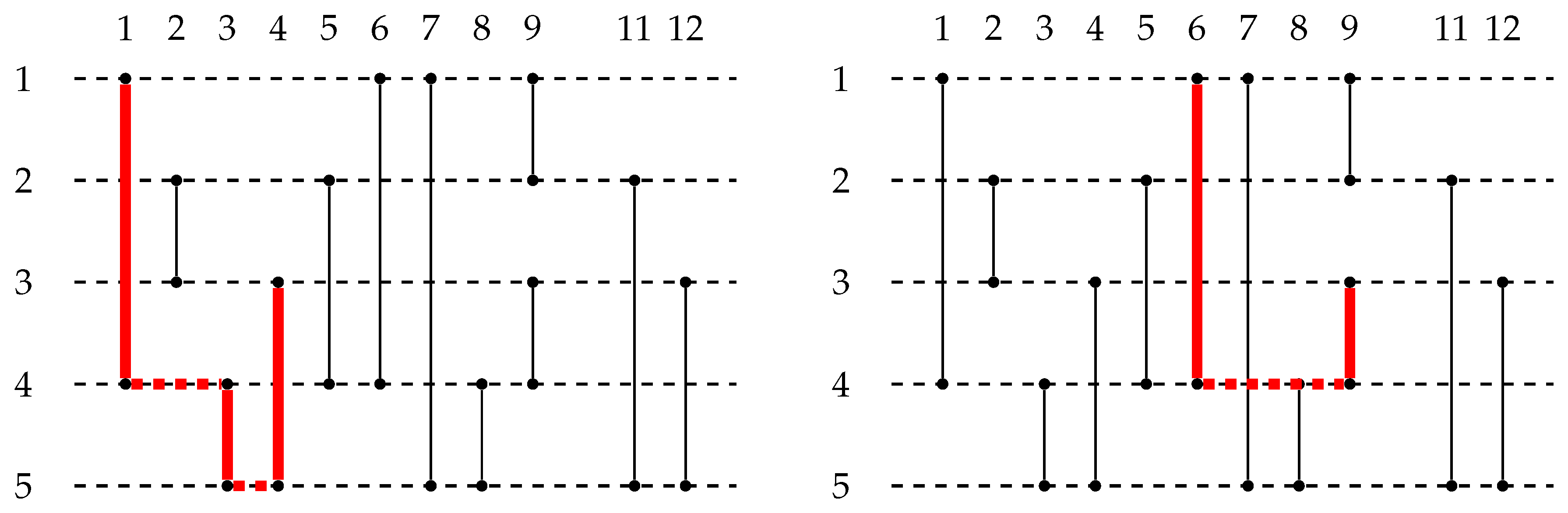
6], if we just remove all time information from the temporal graph (and collapse, if necessary, multiple edges between any two vertices into a single edge), we clearly lose all the temporal information of the graph. This loss can be critical to the understanding of the reachability relationships between the nodes of the graph. For example, In the left part of
Figure 1, a temporal network with five nodes and five temporal edges is represented, while, In the right part of the figure, the “non-temporal” version of the graph (In which all edge temporal labels have been removed) is shown. It is easy to verify that the two simple paths from node 1 to node 2 in the non-temporal graph do not exist in the temporal network (a temporal path is, intuitively, a path such that each edge in the path appears later than the edges preceding it in the path). Indeed, the edge from node 3 to node 2 appears at time 1, hence it cannot be used within a path starting from node 1, since all of this node’s edges appear after that time. Moreover, the path of length 2 from node 1 to node 5 in the non-temporal graph does not exist in the temporal graph since it is only possible to reach node 3 from node 1 in one step at time 5, while the edge from node 3 to node 5 appears at time 4. In summary, removing temporal information may let us conclude that two nodes (i.e., 1 and 2) are reachable, while they are not, or that the length of the shortest path between two nodes (i.e., 1 and 5) is smaller than it really is.
For this reason, we are interested in developing algorithmic techniques that allow us to efficiently compute aggregate information about temporal paths and time-distances between pairs of nodes. In particular, we focus on the
temporal neighborhood function (in short,
tnf) of a temporal network, which is the natural extension of the neighborhood function already widely analyzed in the case of non-temporal graphs [
7,
8]. More precisely, given a time interval
, the temporal neighborhood function returns the value
, where
denotes the set of pairs of nodes
such that there exists a
temporal path from
u to
v, which starts from
u not earlier than
, arrives in
v no later than
, and it is such that each edge appears later than the edges preceding it.
By assuming that a temporal network is represented by the sequence of its temporal edges, ordered in non-decreasing order with respect to their appearance times, the temporal neighborhood function can be easily computed by making use of the following “scan-based” algorithm [
9], which allows us to compute the cardinality of the
temporal cone of a node
s, which is the set of nodes reachable from
s in the interval
.
Initialize and for all .
For each (directed) edge :
- (a)
If , , and , then .
- (b)
If , then stop.
Return the number of elements of t different from ∞.
If m is the number of temporal edges, it is easy to verify that the complexity of the above algorithm is . In order to compute the temporal neighborhood function, we have to execute the above procedure starting from every node of the temporal network. We refer to this algorithm as etnf (Exact tnf). Hence, if n denotes the number of nodes, we can conclude that etnf runs in time .
Unfortunately, this time complexity is not acceptable when dealing with real-world temporal networks, where there are millions of nodes and billions of temporal edges. For this reason, In this paper, we propose a new algorithm called atnf for approximating the temporal neighborhood function of a temporal network.
1.1. Our Results
In order to approximate the temporal neighborhood function, we first describe a simple dynamic programming algorithm for computing the
reverse temporal cone of a node
s, which is the set of nodes that can reach
s in a specific interval
. Note that, if we can compute the cardinalities of the reverse temporal cones, then we can also compute the temporal neighborhood function. We then show how the
sketch approach, which has already been widely used in the case of non-temporal graphs [
10,
11,
12,
13], can be applied to the case of temporal networks in order to approximately compute the cardinalities of the reverse temporal cones of a temporal network. More specifically, the resulting approximation algorithm, called
atnf (Approximated
tnf), has a relative error bounded by
with high probability, whenever the sketches have size
. The time complexity of the algorithm is
.
We then experimentally evaluate the quality of the approximation performed by atnf by comparing the approximate value of the temporal neighborhood function with the exact one (computed by making use of the scan-based exact algorithm described in the previous section) on a data-set containing several medium-size temporal networks. As a matter of fact (and as expected), the obtained approximation is much better than the one guaranteed in theory, even when the size of the sketches is significantly smaller than the required size. By making use of the approximation algorithm, we hence show how we can accurately approximate, In a few minutes, the temporal neighborhood function (and, hence, the distance distribution) of two large temporal networks: the IMDB collaboration network (which is undirected) and the Twitter re-tweets network (which is directed). The first network contains more than half a million nodes and more than three million edges, while the second network contains more than two million nodes and more than sixteen million edges.
Finally, we apply
atnf in order to analyze and compare the behavior of twenty-five public transportation temporal networks [
14]. In particular, we analyze the reachability properties of these networks, by computing the values of the temporal neighborhood function in different intervals during a day. As a matter of fact, we observe that there are cities which perform significantly better than others with respect to these reachability properties, and that this result cannot always be deduced by simply looking at the density of the temporal network. Moreover, we show that the quality of the approximation is preserved even with small values of the sketch sizes: this allowed us to perform the entire experimental evaluation for all the cities in less than one hour (while the exact algorithm would have roughly required almost four days).
1.2. Related Work
Algorithms for distance computation in temporal networks have been proposed in [
6,
15]. The method in [
16] uses a similar algorithm to [
6] for computing spanning trees. The method in [
9] proposes to index data to answer reachability and path queries in temporal networks. The problem of finding different types of path (minimum traveling time, earliest arrival time, and minimum number of hops) in the temporal network has also been investigated in a distributed context [
17].
A problem related to the one analyzed in this paper is computing distances in road networks, where edges have a traversal time but are supposed to exist at all times. In this case, the focus is mainly on pre-computing some information in order to be able to answer fastest path queries very quickly (see, for example, [
18,
19]). The analysis in [
20] focuses on the impact of the passenger demand on the performance of path finding algorithms.
Concerning public transportation networks, many works have focused on the efficient design of such networks, by considering, e.g., where to place hubs, see, for instance [
21,
22], or on their
robustness or
resilience, by studying how perturbations on specific nodes or links, or changes in demand, affect the whole network; see, for instance, [
23,
24]. Other works have used connectivity notions to evaluate the importance of nodes in transportation networks; see, for instance, ref. [
25] and references within.
1.3. Structure of the Paper
In
Section 2, we give all basic definitions and notations concerning temporal networks, paths, cones and neighborhood functions. In
Section 3, we describe the dynamic programming algorithm for computing reverse temporal cones, and we show how the bottom-
k sketch approach can be used in order to approximate the cardinalities of these cones (and, hence, the temporal neighborhood function), getting our approximation algorithm
atnf. In
Section 4, we experimentally evaluate the quality of the approximation of
atnf and its running time, comparing our results with the ones of
etnf. Moreover, we use the algorithm itself to compute the temporal neighborhood functions of two large temporal networks. Finally, In
Section 5, we apply
atnf for comparing the reachability properties of twenty-five public transportation networks.
3. Computing Temporal Neighborhood Functions through Reverse Temporal Cones
As we already said, In this paper, we consider the left-to-right order for reading the stream of temporal edges, which corresponds to reading the edges in non-decreasing order with respect to their appearing times.
Definition 4. Given a temporal graph and a time instant , thepredecessor of t in G is the maximum time instant such that (if does not exist, then we set ).
For example, by referring to the temporal graph of
Figure 2,
,
, and
.
Observe that, if and , then contains exactly all pairs of nodes such that any earliest arrival path from u to v satisfies .
In order to compute the temporal neighborhood function of a temporal graph G in a given time interval , we first introduce the following definition.
Definition 5. Given a temporal graph , a node u, and a time interval , the reverse temporal coneof u in the interval is defined as .
In other words, the reverse temporal cone of u in the interval contains all nodes v that can reach u in (hence, if , then ). The advantage of referring to reverse temporal cones is that these cones can be easily computed by using the following dynamic programming algorithm (observe that, for any , is the neighborhood of u at time t, that is, the set of nodes v such that ).
Base case.
Recursive step Let with and suppose we have computed for every with . Then, .
The base case simply states that, if there is an edge
, then
v belongs to the reverse temporal cone of
u in the interval
. The recursive step, instead, says that, if there is an edge
, then all nodes that could reach
v before
t can now also reach
u at time
t. For example, by referring to the temporal graph of
Figure 2 (in which all edges are bidirectional),
Table 1 shows the evolution of the reverse temporal cones
according to the above algorithm (until all nodes are reachable from all other nodes).
Let us assume that the set of temporal edges of a temporal graph is ordered in non-decreasing order with respect to the appearing times, and that edges are not bidirectional. Let be the resulting ordered set of temporal edges, so that the appearing time of is not greater than the appearing time of , for any i with . We can then implement the above dynamic programming algorithm by scanning the edges in one after the other. For each edge , if , then we add v to . Otherwise (that is, ), we set equal to the union of and , after having initialized to the first time an edge appearing at time t is scanned. Since the size of the intermediate reverse temporal cones can be linear in the number n of nodes in the graph, the time complexity of this algorithm is . Moreover, if we want to maintain all the intermediate reverse temporal cones, then the space complexity of the algorithm is . However, if we just want to compute the final reverse temporal cones, then the space complexity can be reduced to . Observe that, if the edges are bidirectional, then we can easily modify this algorithm by simply considering twice each edge : once as , and the other as .
Once we have computed the reverse temporal cones in a specific interval
, we can easily compute
. Indeed, we have that, for each pair of nodes
u and
v,
belongs to
if and only if
. This implies that
Hence, the temporal neighborhood function can be computed by using the sizes of the reverse temporal cones.
Remark 1. Note that the above dynamic programming approach does not seem to be applicable to the computation of temporal cones, as defined in the previous section. More precisely, it is not clear how to rewrite the recursive step of the algorithm, when referring to temporal cones. Indeed, In general, it holds thatsince, for each vertex v, is the set of all the vertices reachable from v through temporal paths which use edge appearing times smaller than t. Hence, does not necessarily include the nodes in , as the corresponding paths might turn out to be not valid from a temporal point of view. Indeed, the edge from u to v appears at time t, but the edges on the paths from v to other vertices may have appearing times smaller than t. Let us consider, for example, the temporal graph with the three nodes 1, 2, and 3, and the two temporal edges and . Clearly, and . Hence, when the edge is analyzed, we have that 3.1. Approximating the Size of the Reverse Temporal Cones
As we have already observed, the time complexity of the dynamic programming algorithm for computing the reverse temporal cones is , where and . This complexity can turn out to be prohibitive when dealing with temporal graphs with thousands of nodes and millions of temporal edges. For this reason, In this section, we propose atnf, an algorithm for computing an approximation of the size of the reverse temporal cones, which is based on the application of the sketch techniques: these techniques allow us to represent the reverse temporal cone for each node u in a compressed approximated form of (almost) constant size k (typically ). By using cone sketches in place of real cones, we will obtain a dynamic programming approximation algorithm whose time complexity is time.
3.1.1. Sketch Operations
Given a set A, a sketch is a compressed form of representation of A of size , with , providing the following operations.
INIT How a sketch for A is initialized.
UPDATE How a sketch for A is modified when an element u is added to A.
UNION Given two sketches for A and B, provide a sketch for .
SIZE Estimate the number of distinct elements of A.
The following two requirements are needed for sketches: (i) given two sketches and for any two sets A and B, can be computed just by looking at and , and (ii) the order in which the elements are added and adding any element twice does not affect the sketch. We assume that .
3.1.2. Bottom-k Sketches
One of the most popular sketch techniques is the bottom-k technique, which works as follows. Given a mapping and a subset A of U, we denote as the first k elements of A according to r (or A itself if ). A bottom-k sketch for A is .
INIT: .
UPDATE: return .
UNION: return .
SIZE: If return . Otherwise, return .
As an example, let
U be the set of the 26 letters of the alphabet and let
be the following function:
Let
,
, and
. Then,
is
and
is
, as these letters are the three elements of
A and
B, respectively, having minimum
r-values. Hence,
The size of
, which is equal to 10, can then be estimated as follows:
It can be shown that the mean relative error of the sketch sizes with respect to the real sizes is bounded by
and that, if we choose
, the mean relative error is bounded by
with high probability [
10,
11].
3.1.3. Applying Sketches to Reverse Temporal Cones
In the case of reverse temporal cones, the sets whose sizes we want to approximate are the reverse temporal cones at different time instants within a specific time interval
. Indeed, for each edge scanned by the dynamic programming algorithm described in the previous section, either we use the
UPDATE operation in order to add a node to the sketch of a reverse temporal cone, or we use the
UNION operation in order to compute the union of the sketches of two reverse temporal cones. Whenever all edges whose appearing time is in
have been read, we can use the
SIZE operation in order to estimate, for each node
u, the size of
. Let
denote the obtained estimate of
. Hence,
atnf approximates
by using the estimates
as follows:
By linearity of expectation, the approximation performed by atnf is unbiased and has relative error bounded by with high probability, whenever .
4. Experimental Results
This section is devoted to analyze the performance of atnf on approximating . We evaluate both the running time of atnf and the quality of the approximation achieved, comparing our results with the ones provided by etnf. Summarizing, the two algorithms we are going to compare are the following:
atnf Our method for approximating the earliest arrival reverse temporal cones and hence
, as described in
Section 3.1. As the quality of the approximation of
atnf and its running time depend on the value of
k, we analyze the behaviour of
atnf varying
k in the set
.
etnf The method in [
9] described in
Section 1 to compute exactly the earliest arrival temporal cones and hence
for any
.
Implementation and Computing Platform
Our computing platform is a machine with Intel(R) Xeon(R) CPU E5-2620 v3 at 2.40 GHz, 24 virtual cores, 128 GB RAM, and running Ubuntu Linux version 4.4.0-22-generic (machine available at Dipartimento di Informatica, Università di Pisa, Italy). The code has been written in Java, using Java 1.8, for both of the competitors.
Dataset
In order to perform our experiments, we used the following temporal graphs (other temporal networks will be considered in
Section 5, in which we will perform a case study based on the directed public transport networks of 25 cities):
The dimensions of the above temporal graphs are summarized in
Table 2, where we report for each graph its number of nodes and its number of edges, and whether the graph is directed or not. For a given network
G, let
and
denote the minimum and maximum appearing time, respectively, of the temporal edges included in
G. We have then considered different intervals
, for increasing values of
with
, where
is the time horizon of
G (that is, the union of all the appearing times of its temporal edges). Both
etnf and
atnf compute (or approximate) the number of pairs of nodes
u and
v such that, starting from
u not before time
, we can reach
v within time
. As a result, we get an exact cumulative frequency distribution, running
etnf, and its approximation, running
atnf.
Section 4.1 is devoted to measure the quality of this approximation, while
Section 4.2 shows the running times.
4.1. Quality of the Approximation
In order to evaluate the quality of the approximation, for each
, we have compared the approximation
provided by
atnf with respect to the exact value
provided by
etnf, using the
relative error. We have hence considered the
mean relative error (in short,
mre) among all the intervals
for all values of
in
. More formally, the
mre is defined as follows:
For each
, we have repeated the experiments ten times, and we have reported our results in
Table 3. In this table, for each
k, we have reported the average
mre, denoted as
, and the standard deviation, denoted as
, over the ten experiments (note that both
and
are 0 for the
rollernet network, whenever
, since the graph has less than 64 nodes and hence
atnf turns out to always compute the exact values).
In general, both and consistently decrease while increasing k. For , 4, and 8, the average mre appears to be quite large: for , the mre can be up to , and, for , the mre can be close to . By increasing k to 16, we get an average mre consistently smaller than , which further reduces with and , where, in both of the cases, the average mre is very often below . Finally, for , the average mre appears to be always smaller than . For the sake of completeness, looking at the values of , we can observe how the variability of the experiments is more controlled when k increases.
Note that, in the table, the imdb-all and twitter networks are missing since, according to our estimate and as shown in the next section, etnf would have taken more than one week for the first and more than 190 days for the second to complete. Hence, for these two graphs, no quality comparison was possible.
4.2. Running Time and Time Comparison with Respect to etnf
Table 4 reports the average running time (in milliseconds) of
atnf and of
etnf, respectively, to get the approximate and the exact value of
for each
. Increasing the value of
k, the running time of
atnf increases consistently (as also the quality of the approximation). In the case of bigger graphs, the running time of
atnf is orders of magnitude smaller with respect to the one of
etnf (rightmost column). We have highlighted this improvement in
Table 5, where we have shown the ratio between the running time of
atnf and the one of
etnf.
Concerning the smaller graphs, like rollernet and enron, which have respectively 63 and 150 nodes, we have observed that atnf turns to be exact if k is set to a value greater than this number of nodes. In the case of rollernet, it is interesting to note that the dynamic programming algorithm (which, hence, is exact for or 128) is strictly faster than the BFS approach implemented by etnf. On the other hand, as in the case of enron, the running time of atnf, although not exact, can be sometimes worse than the one of etnf whenever the graph has few nodes.
In the general case, running atnf with , and thus getting an average mre below 5.3% (as we have seen in the previous section), the running time of atnf is very often below the running time of etnf. This improvement is even more striking for bigger graphs, where the running time of atnf further reduces to .
For the two biggest graphs, i.e.,
imdb-all and
twitter, we were not able to run
etnf, due to the large amount of time required by the method. For this reason, we have estimated its running time (reported with † in
Table 4). The estimation is based on the fact that
etnf runs
n single-source procedures, each one from a different source node. It is possible to estimate the average running time
of a single-source procedure, sampling
sources and computing the average time
. It is easy to show that this is an unbiased estimator and that, by using the Hoeffding’s inequality,
is bounded with high probability by
, where
r is an upper bound on the maximum time needed by a single-source procedure, e.g., the time for visiting all the edges. By multiplying
by
n, we get an estimation of the running time of
etnf. We have verified experimentally that the order of magnitude reported by our estimation is consistent with the actual time used by
etnf for the smaller graphs. As a result, applying our estimation for the biggest graphs, since a single-source procedure requires on average 1.18 s for
imdb-all and 7.33 s for
twitter, with relative standard deviation, respectively, of 17.49% and 10.87%,
etnf requires 622,185 s (more than a week) for
imdb-all and 25,771,840 s (more than 198 days) for
twitter. On the other hand, setting
,
atnf is able to approximate
in only 112 s for the former graphs and in 71 min for the latter one, as shown in
Table 4. Comparing these running times with our estimates (last two rows of
Table 5),
atnf turns out to be four orders of magnitude faster than
etnf.
5. Case Study: Comparison of 25 Public Transport Networks
In this section, we will show how the
atnf algorithm for computing the approximation of the temporal neighborhood functions can be applied in order to perform an exhaustive analysis of some reachability properties of several temporal graphs in a very efficient way. In particular, we will make use of a recently published collection of 25 cities’ public transport networks [
14]. This collection is available in multiple formats including the temporal edge list for a specific day, which is the format we use here. The list of the 25 cities is summarized in
Table 6, where, for each city, we provide the number of stops (that is, the number of vertices of the temporal graph), the number of temporal edges, the day in which the data were collected, and the radius
R around the city’s central point that should cover all the continuous and dense parts of the city and its public transport network [
14]. We have grouped the 25 cities into five groups according to the vale of
R. In particular, group
i contains all the cities such that
, for
.
Our goal is to analyze the
reachability efficacy of each public transport network. To this aim, we compute the (approximate) value of the temporal neighborhood functions corresponding to different time intervals of the day in which the data were collected. In particular, we divide the interval between 6:00 a.m. and 9:00 p.m. into 30, 15, and 10 intervals of length 30, 60, and 90 min, respectively. For each interval
, we compute the approximate value of the temporal neighborhood function
(normalized with respect to the number of all possible pairs of nodes), by using the
atnf algorithm. In the following, we will represent the distributions of these values by
reachability diagrams such as the one shown in
Figure 5, which refers to the city of Adelaide.
Observe that, in the case of transport networks, going from one stop to another, i.e., following an edge, takes some time. Therefore, in our dataset, the temporal edge list contains the starting time
and the arrival time
of each temporal edge
e between two nodes
u and
v. In order to apply our approach, we have used the following transformation. For each edge
e in the dataset from
u to
v with starting time
and arrival time
, with
, we have replaced
e with a pair of two edges: one from
u to
with appearing time
, and the other from
to
v with appearing time
, where
is a new dummy node. For the edges
e from
u to
v in the dataset such that
, we replace
e by an edge from
u to
v with appearing time
. It is easy to show that there is a one-to-one correspondence between the feasible journeys in the original dataset and the sequences induced by the non-dummy nodes in the temporal paths of the resulting temporal graph. Moreover, it is worth remarking that, when computing the temporal neighborhood function in our transformed temporal graph, we have to focus only on non-dummy nodes. To this aim, we have slightly modified our approach in order to exclude the dummy nodes from the sketches of our reverse temporal cones and, hence, not to count them in the final estimation of the temporal neighborhood function. In particular, to do this, in the base case in
Section 3, it is enough to exclude
u from
, whenever
u is a dummy node.
In the left column of
Figure 6, we show, for each city group, the reachability diagrams of all cities in the group in the case in which we consider intervals of 60 min (these diagrams have been obtained by running 20 times the approximation algorithm with
, and by taking the average values). As can be seen, in the case of the first and the last group, the two cities included in the group behave quite similarly, even if the city of Sydney seems to be more efficient in correspondence with the two peaks of its diagram at 8:00 a.m. and at 5:00 p.m. (which might be considered as the rush hours of the day). In the other three groups, instead, there is clearly a city more efficient than the others of the group (that is, Luxembourg in Group 2, Berlin in Group 3, and Adelaide in Group 4). In each of these groups, the existence of a second more efficient city (that is, Palermo, Winnipeg, and Paris) is also evident. While, in Group 2, two cities (that is, Rome and Rennes) fight for the third position, in Group 3, all of the other cities are basically equivalent.
Note that we are not evaluating the whole quality of a public transport service, which of course depends on many other factors, such as robustness, safety, reliability, and customer service; instead, we are only comparing different public transport networks in terms of their temporal neighborhood functions during a day. In particular, the reachability diagram of a public transport network should only be interpreted as an indicator of the percentage of the pairs of nodes that are connected in each interval, with respect to the total number of pairs of nodes. It is also worth emphasizing the fact that, in order to use these diagrams for comparing two public transport networks of two cities, we must implicitly assume that the nodes of a network are uniformly spread in the circle of radius R corresponding to the network itself. It clearly does not make sense to compare a transportation network in which nodes are concentrated in a small sector of the circle with one in which nodes are uniformly spread, since this would turn out into a greater efficiency of the first network with respect to the second one. Unfortunately, we are not able to verify that nodes are uniformly spread in the circle, and we can only assume that this requirement is satisfied.
One could suspect that results similar to the ones shown in the left column of
Figure 6 could be obtained by simply considering the temporal density of the original transport networks. For each interval
, let
denote the number of edges from
u to
v with both starting and arrival time in
. We then define the temporal density in the interval
as
, where
n denotes the number of nodes of the network. In the right column of
Figure 6, we show, for each city group, the
density diagrams of all cities included in the group. As it can be seen, in Groups 1, 2, 3 and 5, the first city is the same as in the reachability diagrams. In Group 4, instead, Paris seems to have the densest public transport network, even if it is not the first city in terms of reachability cone sizes. Moreover, while the reachability and the density diagrams of Groups 1 and 5 seem to be quite consistent, this is not the case for Groups 2 and 3. For instance, in Group 2, Rome is denser than Palermo, but Palermo outperforms Rome in terms of reachability, while, in Group 3, this phenomenon happens in the case of Prague and Winnipeg. In other words, the reachability diagram seems to provide some information that is not explicitly given by the density diagram. It is also worth observing how several cities present two peaks in their reachability and density diagrams, which we can assume correspond to the two rush hours of the day. This seems to indicate that these cities, in correspondence with these rush hours, increase the number of connections and provide a better service in terms of the number of pairs of connected nodes.
In
Figure 7, instead, we compare the reachability diagrams of the five groups obtained with time intervals of length 30 and 90 min, respectively (these diagrams should also be compared to the reachability diagrams shown in the left column of
Figure 6, which are obtained with time intervals of length 60 min). It is worth observing that, in the second and in the third group, considering shorter time intervals makes the city with the better diagram perform even better compared to the others, and it basically nullifies the differences among the other cities. When larger time intervals are analyzed, it seems that the only effect we get is that the reachability diagrams are systematically shifted up. This is quite reasonable, since we can expect that, in a time interval of one hour and half, a significant percentage of all possible pairs of nodes are now connected. It is anyway worth noting that, in the case of the three cities in Group 4 and of the two cities in Group 5, even with time intervals of 90 min, this percentage is quite low (less than
in Group 4 and less than
in Group 5). This suggests that, in order to obtain a globally almost total connectivity, these cities require trips of quite great duration.
Finally, in
Figure 8, we show the reachability diagrams of three sample cities obtained with different values of
k in
atnf (the number of experiments is always 20). As it can be seen, the diagrams are almost identical, which might suggest that even
could be used in order to reduce the execution time. However, we decided to use
in the previously described experiments in order to further increase the approximation quality of the results.
As we said at the beginning of this section, the main goal of this analysis has been to describe a case study in which, by using
atnf, we can extremely reduce the total execution time of the experiments. For example, with
and 20 experiments, producing the reachability diagrams of all cities with respect to intervals of 60 minutes in length requires approximately
hours. The time to get the exact values of the temporal neighborhood functions for each time interval by using
etnf is instead approximately equal to
hours, that is, between one and two orders of magnitude bigger than the running time of
atnf, consistently with the results shown in
Section 4.
6. Conclusions
In this paper, we have proposed a new algorithm for approximating the temporal neighborhood function of a temporal network, which is based on the bottom-k sketch technique. We have experimentally validated the quality and the time performance of our algorithm, by comparing it with a recently proposed scan-based algorithm. We showed that our algorithm is able to obtain good quality results (typically with a mean relative error of 5% or less) in a very small fraction of the time of the exact algorithm (typically 0.3% or less). Finally, we have applied our algorithm to the analysis of the reachability properties of 25 public transport networks and showed that the neighborhood function gives some non-trivial insight about the number of pairs of stops that are reachable from one another.
From a more technical point of view, a quite natural and straightforward extension of our work consists of applying other sketch techniques, such as, for example, the ones based on the probabilistic counting approach [
7,
8,
38]. We are confident that, by using these other techniques, our results can be improved both in terms of approximation quality and of execution time. A comparison of the different sketch techniques for approximating the temporal neighborhood function is beyond the scope of this paper, whose main goal is showing how these techniques are extremely effective when applied to temporal networks.
More interestingly, the approach we have described in this paper can also be applied to compute a different kind of temporal cones. Intuitively, these cones would allow us, for each node u of a temporal graph , to determine what is the latest starting time from any other node v that can reach u in a specified interval , in order to arrive at u not later than . By appropriately adapting the dynamic programming algorithm for computing the reverse temporal cones, we can show that the latest starting time cones can also be computed in time and space (or if we do not need to store all the intermediate results). Moreover, in order to improve the efficiency of the algorithm, we can use, even in this case, the bottom-k sketch technique, exactly as we have done in the case of the reverse temporal cones.
Finally, a more general question is whether other heuristics can be used in order to compute graph metrics for which the sketch approach does not seem to be very efficient in the case of classical graphs. For example, a promising research direction is to define an analogue of the backward breadth-first search for temporal networks, in order to apply techniques that have been extremely powerful for computing the diameter of a graph [
39,
40] or to apply sampling techniques for computing centrality measures in temporal networks [
41,
42].


