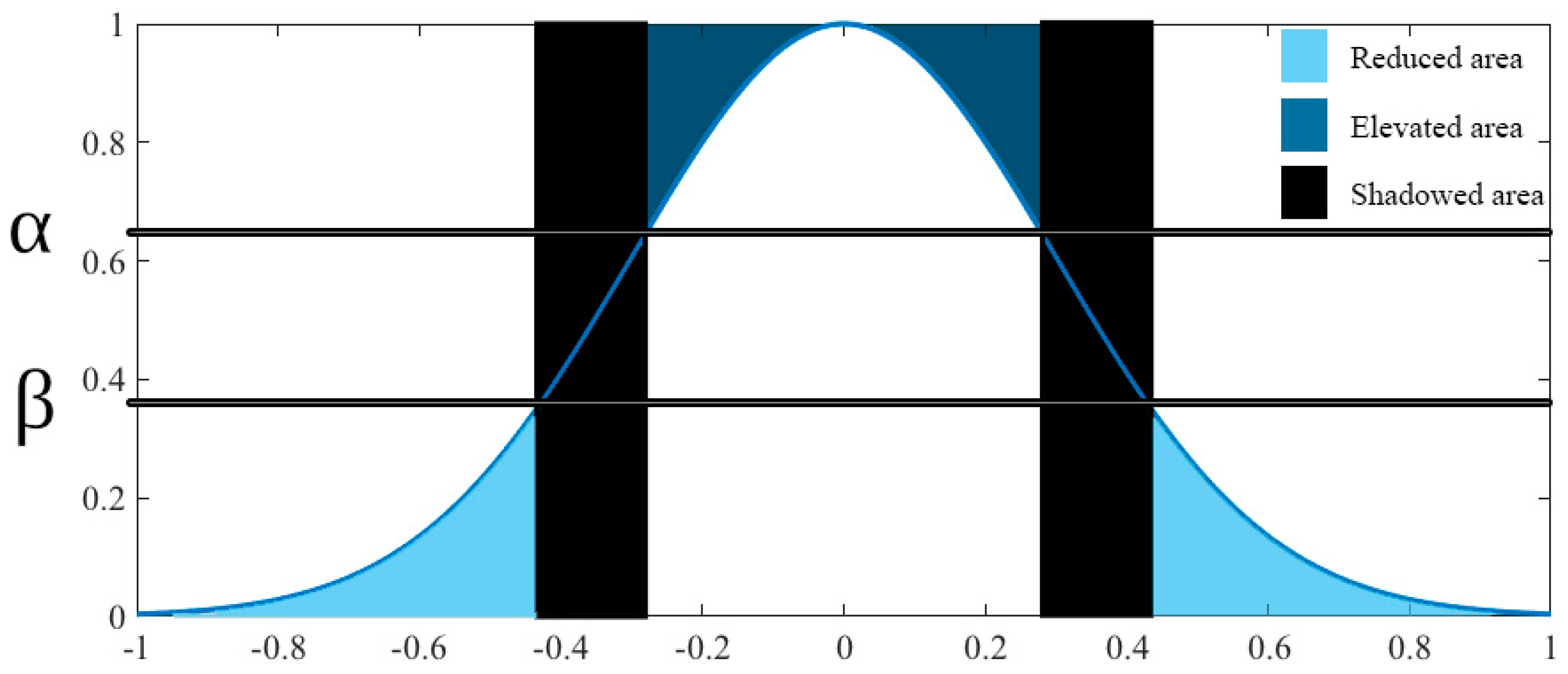
Article

Shadowed Type-2 Fuzzy Systems for Dynamic Parameter Adaptation in Harmony Search and Differential Evolution Algorithms

Tijuana Institute of Technology, Calzada Tecnologico s/n, Fracc. Tomas Aquino, Tijuana 22379, Mexico
*
Author to whom correspondence should be addressed.
Algorithms 2019, 12(1), 17; https://doi.org/10.3390/a12010017
Submission received: 22 November 2018 / Revised: 11 December 2018 / Accepted: 3 January 2019 / Published: 9 January 2019
(This article belongs to the Special Issue Metaheuristic Algorithms in Optimization and Applications (volume 2))

Abstract

:
Nowadays, dynamic parameter adaptation has been shown to provide a significant improvement in several metaheuristic optimization methods, and one of the main ways to realize this dynamic adaptation is the implementation of Fuzzy Inference Systems. The main reason for this is because Fuzzy Inference Systems can be designed based on human knowledge, and this can provide an intelligent dynamic adaptation of parameters in metaheuristics. In addition, with the coming forth of Type-2 Fuzzy Logic, the capability of uncertainty handling offers an attractive improvement for dynamic parameter adaptation in metaheuristic methods, and, in fact, the use of Interval Type-2 Fuzzy Inference Systems (IT2 FIS) has been shown to provide better results with respect to Type-1 Fuzzy Inference Systems (T1 FIS) in recent works. Based on the performance improvement exhibited by IT2 FIS, the present paper aims to implement the Shadowed Type-2 Fuzzy Inference System (ST2 FIS) for further improvements in dynamic parameter adaptation in Harmony Search and Differential Evolution optimization methods. The ST2 FIS is an approximation of General Type-2 Fuzzy Inference Systems (GT2 FIS), and is based on the principles of Shadowed Fuzzy Sets. The main reason for using ST2 FIS and not GT2 FIS is because the computational cost of GT2 FIS represents a time limitation in this application. The paper presents a comparison of the conventional methods with static parameters and the dynamic parameter adaptation based on ST2 FIS, and the approaches are compared in solving mathematical functions and in controller optimization.

1. Introduction

Nowadays, metaheuristic optimization methods represent a very interesting alternative for the optimization of complex problems without the mathematical modeling of the problem, and they have been successfully applied in several kinds of application, for example, in control applications [1,2,3], optimizing Artificial Neural Networks [4,5,6], optimizing a controller applied in an complex electromechanical process [7], fuzzy controllers [8,9], etc. On the other hand, dynamic parameter adaptation in metaheuristic methods based on fuzzy logic can improve their optimization performance as can be observed in [10,11,12,13]. However, this dynamic adaptation based on fuzzy logic significantly increases the computational cost of the optimization process. There are some works where the dynamic adaptation of metaheuristic parameters is realized through Interval Type-2 Fuzzy systems, for example, in [2,3], and in some works, this adaptation is successfully realized by General Type-2 Fuzzy Systems. However, the main limitation of applying Type-2 Fuzzy systems, specifically General Type-2 Fuzzy Sets, for the dynamic adaptation of metaheuristic parameters, is the higher computational cost.
The computational cost of Interval Type-2 Fuzzy Systems is nearly double that of Type-1 Fuzzy Systems, and the computational cost of General Type-2 Fuzzy Systems depends on the representation used for modeling the system, for example, using the α -planes representation, the computational cost is directly proportional to the number of α -planes used in approximating the model. In this case, the approximation improves accuracy by increasing the number of α -planes, in other words, the computational cost is significantly elevated.
The contribution of the present work is the application of Shadowed Type-2 Fuzzy Systems as a method for approximating General Type-2 Fuzzy Systems modeled with the α -planes representation. The main difference is that the Shadowed Type-2 Fuzzy Inference System (ST2 FIS) approach requires only two α -planes to model the GT2 FIS, but the values of α are selected with the optimization criteria for shadowed sets proposed by Pedrycz in [14], and recent examples of the ST2 FIS applied in control problems can be found in [15]. On the other hand, the optimization of fuzzy controllers that was previously presented, for example in [1,3,10,16], is presented. The reason for exploring this application is because the fuzzy controllers have been proven to have good performance in complex applications, for example, in [17].
The rest of the paper is organized as follows. Section 2 describes type-2 shadowed sets theory, Section 3 shows metaheuristic algorithm concepts, Section 4 explains the dynamic parameter adaptation process, Section 5 summarizes the simulation results, and finally, Section 6 offers the conclusions.

2. Type-2 Fuzzy Systems and Shadowed Sets

With the emergence of Type-1 Fuzzy Inference Systems (T1 FIS) in 1965 [18], computational science achieved the capability to model the vagueness in the real world and create mathematical models that represent human knowledge. Nowadays, fuzzy sets have evolved to GT2 FIS that allows not only a vagueness model, but, in addition, allows an uncertainty modelling approach to be used, and the mathematical expression of the GT2 FIS is denoted in Equation (1):
A ˜ ˜ = { ( ( x , u ) , µ A ˜ ( x ) ) | x X ,   u J x u [ 0 , 1 ] } .
In order to apply the GT2 FIS to real-world applications, some alternatives exist for modeling this system, such as the vertical slices or z-slices representation [19], the Geometric approximation [20] and the horizontal slices or α -planes representation [21]. The present work is focused on the   α -planes representation that consists of discretizing the secondary axis of GT2 FIS in several horizontal slices called α -planes. These α -planes are expressed by Equation (2) and can be computed as an IT2 FIS [22]. Then, with the union of every α -plane, the GT2 FIS is modeled, as described in Equation (3):
A ˜ α = { ( ( x , u ) , α ) | x X ,   u J x [ 0 , 1 ] }
A ˜ ˜ = A ˜ α .
In order to reduce the computational cost of the α -planes representation, the Shadowed Type-2 FIS was introduced in [23]. The proposal focused on modeling the GT2 FIS with only two optimal α -planes, eliminating the excessive precision, and the selection of the optimal α -planes was performed through the concepts that Pedrycz proposed for the shadowed set theory [14,24,25,26].
The basic concepts of shadowed sets consist of realizing two α -cuts on a Type-1 fuzzy set, with α and β values. Based on these α -cuts, three intervals are described, as explained in Equation (4).
S μ A ( x ) = { 1 ,   i f   μ A ( x ) α 0 ,   i f   μ A ( x ) β [ 0 , 1 ] ,   i f   α μ A ( x ) β
These intervals can be interpreted as three regions: the elevated region for the membership degree of 1, the reduced region for the membership degree of 0, and for the shadowed area, the membership degree is in [0, 1]. Based on these regions, Pedrycz proposed that the optimal α and β values can be obtained by the following expression shown in Equation (5):
e l e v a t e d   a r e a ( α , β ) ( μ A ) +   r e d u c e d   a r e a ( α , β ) ( μ A ) = s h a d o w e d   a r e a ( α , β ) ( μ A ) .
The graphical interpretation of Equation (5) can be appreciated in Figure 1.
Then, the optimal α and β values are obtained by the optimization of the V ( α , β ) function described in Equation (6):
V ( α , β ) = | x A r   μ A ( x ) d x + x A e   ( 1 μ A ( x ) ) d x x S   d x | .
In [23], Linda and Manic proposed the use of shadowed sets in the secondary axis of the GT2 FIS, finding, in this way, the optimal α and β values and then using these values as α -planes. In this way, the computational cost is reduced, and the implementation of GT2 FIS for dynamic parameter adaptation in metaheuristic algorithms is allowed.

Trapezoidal ST2 MF

For the present paper, it was decided to use the TrapezoidalG (TrapG) ST2 membership function (MF) introduced in [27] that is based on a Trapezoidal GT2 membership function with a Gaussian membership function as a secondary membership function. The equation of this function is expressed in Equation (7), and its illustration is found in Figure 2.
TrapG   ST 2   MF   = { o { μ ¯ O = μ ¯ t ( x ) + μ _ t ( x ) 2 1.449 | μ ¯ t ( x ) μ _ t ( x ) 10 | μ _ O = μ ¯ t ( x ) + μ _ t ( x ) 2 + 1.449 | μ ¯ t ( x ) μ _ t ( x ) 10 | l { μ ¯ I = μ ¯ t ( x ) + μ _ t ( x ) 2 0.9282 | μ ¯ t ( x ) μ _ t ( x ) 10 | μ _ I = μ ¯ t ( x ) + μ _ t ( x ) 2 + 0.9282 | μ ¯ t ( x ) μ _ t ( x ) 10 |

3. Metaheuristic Algorithms

The metaheuristic algorithms are iterative methods for general purpose search and optimization. They are iterative procedures that intelligently guide a subordinate heuristic by combining different concepts to properly explore and exploit the search space. This section presents two particular metaheuristic algorithms, which are the Harmony Search algorithm [28] and the Differential Evolution algorithm [29].

3.1. Harmony Search Algorithm

The Harmony Search algorithm (HS) was developed by Zong Woo Geem in 2001 [30]. This algorithm is based on the musical composition, specifically of jazz, and has three main components in the improvisation process which are Harmony Memory Accepting (HMR), Pitch Adjustment (PArate) and Random Selection. The HS includes these 5 steps and their respective equations.
Step 1: Initialize the problem and parameters:
Minimize   f ( x ) s . t .     x ( j ) [ L B ( j ) ,   U B ( j ) } ,   j = 1 , 2 , ,   n ] .
Step 2: Initialize the Harmony Memory (HM):
H M = [ x 1 1 x 2 1 x N 1 f ( x 1 ) x 1 2 x 2 2 x N 2 f ( x 2 ) x 1 H M S x 2 H M S x N H M S f ( x H M S ) ] .
Step 3: Improvise a new Harmony:
X n e w ( j ) = X n e w ( j ) ± r   × B W .
Step 4: Update the Harmony Memory:
To update the HM with a new solution vector, x n e w   , the objective function is used to evaluate them. A comparison is made to find out if the new vector solution is better than the worst historical vector solution, and then the worst historical is excluded and substituted with a new one.
Step 5: Check the stopping criteria:
The process is repeated until the number of improvisations (NI) is satisfied; otherwise, the process repeats steps 3 and 4. Finally the best solution is achieved and considered as the best result to the problem. The Harmony Memory Accepting (HMR) parameter represents the intensification or exploitation, the pitch adjustment (PArate), and randomization parameters represent the diversification or exploration of the algorithm.
These components are described in more detail in [31,32,33].

3.2. Differential Evolution Algorithm

Differential Evolution (DE) is a simple and fairly used algorithm that was originally proposed by Storn and Price in 1994 [34] and is mainly composed of the following operations: initialization of the population structure defined by Equations (11)–(16), initialization by Equation (17), mutation expressed by Equation (18), crossover defined by Equation (19), and selection defined with Equation (20).
The way in which this algorithm works is by initializing its population within a search space depending on the problem. Then, three individuals are selected at random and with them, the mutation and crossover operations are performed. The best individual is selected and passes to the next generation and so on until the stopping criterion of the algorithm is met.

3.2.1. Population Structure

The Differential Evolution algorithm maintains a pair of vector populations, both of which contain Np D-dimensional vectors of real-valued parameters. The current population, symbolized by P x , is composed of those vectors, x i , g , that have already been found to be acceptable either as initial points, or by comparison with other vectors:
P x , g = ( x i , g ) ,   i = 0 , 1 , ,   N p 1 ,     g = 0 , 1 , ,   g m a x
x i , g = ( x j , i , g ) ,     j = 0 , 1 ,   , D 1
P v , g =   ( v i , g ) ,   i = 0 , 1 , ,   N p 1 ,     g = 0 , 1 , ,   g m a x
v i , g = ( v j , i , g ) ,     j = 0 , 1 ,   , D 1
P u , g =   ( u i , g ) ,   i = 0 , 1 , ,   N p 1 ,     g = 0 , 1 , ,   g m a x
u i , g = ( u j , i , g ) ,     j = 0 , 1 ,   , D 1 .

3.2.2. Initialization

Before initializing the population, the upper and lower limits for each parameter must be specified. These 2D values can be collected by two initialized D-dimensional vectors, bL and bU, to which the subscripts L and U indicate the lower and upper limits respectively. Once the initialization limits have been specified, a number generator randomly assigns each parameter in every vector a value within the set range. For example, the initial value (g = 0) of the j-th vector parameter is i t h :
x j , i , 0 = r a n d j ( 0 , 1 ) ×   ( b j , U b j , L ) +   b j , L .

3.2.3. Mutation

In particular, the differential mutation adds a random sample equation showing how to combine three different vectors chosen randomly to create a mutant vector:
v i , g =   x r 0 , g + F × ( x r 1 , g x r 2 , g ) .

3.2.4. Crossover

To complement the differential mutation search strategy, DE also uses uniform crossover which is sometimes known as discrete recombination (dual). In particular, DE crosses each vector with a mutant vector:
u i , g =   u j , i , g { v j , i , g   i f   ( r a n d j ( 0 , 1 ) C r   o r   j = j r a n d ) x j , i , g                 o t h e r w i s e .

3.2.5. Selection

If the test vector, u i , g , has a value of the objective function equal to or less than its target vector, x i , g It replaces the target vector in the next generation; otherwise, the target retains its place in the population for at least another generation:
x i , g + 1 =   { u i , g   i f   f ( u i , g )   f ( x i , g ) x i , g   o t h e r w i s e .
The operations of mutation, recombination, and selection are applied repeatedly until the optimal solution is found, or the specified terminating pre-criteria are satisfied.

4. Dynamic Parameter Adaptation

In this section, we explain in detail the structure of the fuzzy system used for each of the HS and DE algorithms. The fuzzy system used for both algorithms has one input and one output. In the case of the HS algorithm, the input parameter is the iterations and for the output, the HMR parameter is used, and for the DE algorithm, the input parameter is the generations and the output parameter is F (mutation). Equation (21) is used to calculate the input of the fuzzy system according to the method:
E x p e r i m e n t =   C u r r e n t   E x p e r i m e n t M a x i m u m   o f   e x p e r i m e n t s .
In Equation (21), the experiment refers to iterations for the FHS method and generations for the FDE method. The current experiment represents the current iterations or generations and the maximum of experiments represents the maximum number of iterations and generations.
The parameters of the outputs mentioned above are converted into fuzzy parameters based on the following Equations (22) and (23):
H M R =   i = 1 r h m r μ i h m r   ( h m r 1 i ) i = 1 r h m r μ i h m r
where HMR is the memory consideration; r h m r is the number of rules of the Shadowed Type-2 Fuzzy System corresponding to hmr; h m r 1 i is the output result for rule i corresponding to hmr; μ i h m r is the membership function of rule i corresponding to hmr.
F =   i = 1 r F μ i F   ( F 1 i ) i = 1 r F μ i F
where F is the mutation; r h m r is the number of rules of the Shadowed Type-2 Fuzzy System corresponding to F; F 1 i is the output result for rule i corresponding to F; μ i F is the membership function of rule i corresponding to F.
Both fuzzy systems in the input and outputs are granulated into three membership functions, as shown in Figure 3 and Figure 4 respectively. They are granulated into low, medium, and high, and the rules are described in Table 1 and Table 2.
The rules are based on previous experimentation as presented in [16,35], and for the ST2FDE method are used in a decreasing fashion and for the ST2FHS method are used in an increasing fashion, respectively.

5. Experiments

The experiments designed to evaluate the proposed approach are divided into two categories: first, the optimization of mathematical functions and secondly the optimization of controllers. Benchmark problems are widely used to validate the appropriate performance of algorithms and their variants. In this case, benchmark mathematical functions and a control problem are used to validate the correct operation of the ST2FHS and ST2FDE methods.

5.1. Mathematical Functions

There are several types of benchmark mathematical function; in this case, the functions chosen for the experiment are summarized in Table 3.
The parameters used for the experimentation are the following: 100 individuals or harmonies, 30 executions, 2000 iterations or generations, and 10, 50 dimensions for most of the functions, except for the Power sum function that only uses 4 dimensions.
The statistical test that is used is the Z-test that is based on Equation (24), and the parameters used for this test are an alpha of 0.05, a level of confidence of 95%, and a sample size of 30. The main goal is to verify that by using the methods for dynamic parameter adjustment with Shadowed Type-2, we can obtain a better result with respect to the original methods for all values lower than −1.645:
Z =   ( X ¯ 1 X ¯ 2 ) ( μ 1 μ 2 ) ( σ 1 σ 2 ) .
Thirty experiments were performed using the HS, DE, ST2FHS, and ST2FDE methods. Table 4, Table 5, Table 6, Table 7, Table 8, Table 9, Table 10, Table 11 and Table 12 summarize the results obtained for the HS and ST2FHS methods, and Table 13, Table 14, Table 15, Table 16, Table 17, Table 18, Table 19 and Table 20 show the results obtained for the DE and ST2FDE methods. In these tables, the best, worst, average, standard deviation, and Z-values obtained for each mathematical function are presented.
The results shown in Table 4 through Table 12 using the set of functions achieve significant evidence using 10 and 50 dimensions for the Sum Square, Zakharov, and Powell functions.
In the Dixon & Price and Levy functions, only significant evidence with 50 dimensions is obtained, and for the Trid function, there is only evidence in 10 dimensions.
The results shown in Table 13 through Table 20 using the set of functions achieve significant evidence using 10 and 50 dimensions for the Zakharov, Dixon & Price, Ackley, and Powell functions. In the Sum Square, Levy, and Trid functions, significant evidence is only found with 50 dimensions.

5.2. Controllers Optimization

As a benchmark control problem it was decided to deal with controlling the angular position of a DC Motor, as this is a non-stable control problem that has been considered in the literature to evaluate controllers, for example, in [36,37,38,39]. The plant is illustrated in Figure 5, and the space-state equations are expressed in Equations (25) and (26), respectively. Table 21 shows the parameters of the motor position.
d d t [ θ θ ˙ i ] = [ 0 0 0 1 b J K L 0 K J R L ] [ θ θ ˙ i ] + [ 0 0 1 L ]
y = [ 1 0 0 ] [ θ θ ˙ i ]

5.2.1. Fuzzy controller

The motor position is regulated with a Type-1 (T1) fuzzy controller, which is composed of two inputs and one output, granulated into trapezoidal and triangular membership functions.
The mathematical expression of the trapezoidal membership function is described in Equation (27), and the triangular membership function is described in Equation (28), and the membership functions parameters are presented in Table 22, and the fuzzy system contains 15 fuzzy rules, which are shown in Figure 6.
t r a p m f ( x , a , b , c , d ) = { 0 ,   x a x a b a ,   a   x b 1 ,   b x c d x d c ,   c x d 0 ,   x d
t r i m f ( x , a , b , c ) = { 0 ,   x a x a b a ,   a   x b c x c b ,   b x c 0 ,   c x
A graphic representation of Table 22 is illustrated in Figure 6. The contents of the fuzzy system are two inputs and one output. The first input, called Error, is composed of three membership functions, both of the edges are of the trapezoidal type, and the central is triangular. The second input, called Error Change, contains five functions of membership, two of the edges are the trapezoidal type, and the three central ones are the triangular type. Finally, the output, called Voltage, contains five functions of membership, two of the edges are the trapezoidal type, and the three central ones are the triangular type.
Figure 7 represents the surface of the fuzzy system for the motor position and Table 23 summarize the rules of the controller.
The proposed ST2FHS and ST2FDE methods are used to optimize the values of the membership functions of the motor position controller in order to minimize the RMSE error described in Equation (29). Figure 8 shows the vector that represents the information of the individuals.
RMSE =   1 N t = 1 N ( x t   x ^ t ) 2
The vector contains the information of each individual; the latter represents each position of the triangular or trapezoidal membership function. In total, there are 44 positions of which 25 are fixed and 20 are optimized. The limits of the positions that are optimized are shown in Table 24.
Table 25 and Table 26 show the results obtained by optimizing the parameters of the DC Motor controller, with the ST2FHS and ST2FDE methods, respectively. The noise applied to this controller is 0.5 (Gaussian random number).
Figure 9 and Figure 10 illustrate the best results obtained with the HS method without noise and with noise respectively, Figure 11 and Figure 12 illustrate the best controller surface.
Figure 13 and Figure 14 illustrate the best results obtained with the DE method without noise and with noise, respectively. Figure 15 and Figure 16 illustrate the best controller surface.
It is noticeable in Figure 13 and Figure 15 that the proposed approach obtains a better performance than the conventional approach. However, in order to validate this, a statistical test is realized. Based on the parameters of the z-test statistic presented in Section 5.1 and Equation (24), the results of the Z-values are presented in Table 27.
The Z-values obtained for the statistical test demonstrate the improvement of the proposed approach with respect to the original method.

5.2.2. PID Control

The PID controller (Proportional-Integral-Derivative) is a feedback control mechanism that is widely used in industrial control systems, for example, in [40,41,42]. The PID control algorithm uses three different parameters: the proportional (kp), the integral (ki), and the derivative (kd) gains. The proportional value depends on the current error. The integral depends on past errors, and the derivative is a prediction of future errors. The sum of these three actions is used to adjust the process by means of a control element, such as the position of a control valve or the power supplied to a heater. The general PID algorithm is expressed in Equation (30):
r   ( t ) = M V   ( t ) = K p   e ( t ) + K i   o t e   ( t )   d t + K d   d e ( t ) d t .
In this case, the PID angular position of the motor is used, the ST2FHS and ST2FDE methods are used for the optimization of this control problem, and the control objective is to minimize the settling time. The transfer function for this controller is expressed in Equation (31), and the structure of the control system is shown in Figure 17:
C ( s ) =   K p + K i s + K d s = K d s 2 + K p s + K i s .
Table 28 shows the best parameters obtained from the optimization with the HS, ST2FHS, DE, and ST2FDE methods and the time in which the objective of stabilizing the motor position is achieved. Figure 18 and Figure 19 show the graphical representation of the simulation of these parameters for the HS and ST2FHS, DE, and ST2FDE methods, respectively. Table 29 shows the results for the statistical test.
Figure 18 and Figure 19 show visually similar results, Table 27 contains the results of the values of each PID parameter obtained when using the proposed method, and it can be noted that there is a difference in the settling time between the two methods.
Table 29 presents the statistical test to validate the improvement of the proposed approach with respect to the conventional method.
The Z-values obtained in Table 29 demonstrate that the proposed approach obtains better performance with respect to the conventional approach.

6. Conclusions

In this study, we present the use of a dynamic adaptation of parameters based on the Shadowed Type-2 Fuzzy Inference System theory using the original HS and DE algorithms, which, in this paper, we call ST2FHS and ST2FDE, respectively.
Three case studies were considered. The first was done to obtain the minimum of each benchmark mathematical function using the ST2FHS and ST2FDE methods; the second and third case studies optimized the membership functions of the problem of motor position plant of the engine with the proposed methodology. The difference between the second and third case studies was the type of controller used. For the second case, an FLC was used with noise and without noise and for the third, a PID was used. We can conclude generally and statistically that, for both algorithms, by using the proposed methodology, favorable results were obtained for all cases considered in this paper. The successful implementation of ST2 FIS corresponds to an implementation of an approximation of GT2 FIS; however, with this approach, the computational cost cannot be a limitation in the application of this kind of method in an application that requires several executions.

Author Contributions

Formal analysis, J.S.; Investigation, P.M. and E.O.-R.; Methodology, O.C. and F.V.; Software, C.P.; Validation, P.O.

Funding

This research was funded by Consejo Nacional de Ciencia y Tecnología: 122.

Conflicts of Interest

The authors declare no conflict of interest.

References

  1. Caraveo, C.; Valdez, F.; Castillo, O. Optimization of fuzzy controller design using a new bee colony algorithm with fuzzy dynamic parameter adaptation. Appl. Soft Comput. 2016, 43, 131–142. [Google Scholar] [CrossRef]
  2. Castillo, O.; Amador-Angulo, L.; Castro, J.R.; Garcia-Valdez, M. A comparative study of type-1 fuzzy logic systems, interval type-2 fuzzy logic systems and generalized type-2 fuzzy logic systems in control problems. Inf. Sci. 2016, 354, 257–274. [Google Scholar] [CrossRef]
  3. Olivas, F.; Valdez, F.; Castillo, O.; Gonzalez, C.I.; Martinez, G.; Melin, P. Ant colony optimization with dynamic parameter adaptation based on interval type-2 fuzzy logic systems. Appl. Soft Comput. 2017, 53, 74–87. [Google Scholar] [CrossRef]
  4. Gaxiola, F.; Melin, P.; Valdez, F.; Castro, J.R.; Castillo, O. Optimization of type-2 fuzzy weights in backpropagation learning for neural networks using GAs and PSO. Appl. Soft Comput. 2016, 38, 860–871. [Google Scholar] [CrossRef]
  5. Pulido, M.; Melin, P.; Castillo, O. Particle swarm optimization of ensemble neural networks with fuzzy aggregation for time series prediction of the Mexican Stock Exchange. Inf. Sci. 2014, 280, 188–204. [Google Scholar] [CrossRef]
  6. Saadat, J.; Moallem, P.; Koofigar, H. Training Echo State Neural Network Using Harmony Search Algorithm. Int. J. Artif. Intell. 2017, 15, 163–179. [Google Scholar]
  7. Martin, D.; del Toro, R.; Guerra, R.E.H.; Dorronsoro, J. Optimal tuning of a networked linear controller using a multi-objective genetic algorithm and its application to one complex electromechanical process. Int. J. Innov. Comput. Inf. Control. 2009, 5, 3405–3414. [Google Scholar]
  8. Precup, R.; David, R.; Petriu, E.M. Grey Wolf Optimizer Algorithm-Based Tuning of Fuzzy Control Systems with Reduced Parametric Sensitivity. IEEE Trans. Ind. Electron. 2017, 64, 527–534. [Google Scholar] [CrossRef]
  9. Vrkalovic, S.; Lunca, E.-C.; Borlea, I.-D. Model-Free Sliding Mode and Fuzzy Controllers for Reverse Osmosis Desalination Plants. Int. J. Artif. Intell. 2018, 16, 208–222. [Google Scholar]
  10. Peraza, C.; Valdez, F.; Melin, P. Optimization of Intelligent Controllers Using a Type-1 and Interval Type-2 Fuzzy Harmony Search Algorithm. Algorithms 2017, 10, 82. [Google Scholar] [CrossRef]
  11. Peraza, C.; Valdez, F.; Castillo, O. Study on the Use of Type-1 and Interval Type-2 Fuzzy Systems Applied to Benchmark Functions Using the Fuzzy Harmony Search Algorithm. In Fuzzy Logic in Intelligent System Design; Melin, P., Castillo, O., Kacprzyk, J., Reformat, M., Melek, W., Eds.; Springer: Cham, Switzerland, 2018; Volume 648, pp. 94–103. [Google Scholar]
  12. Liu, J.; Lampinen, J. A Fuzzy Adaptive Differential Evolution Algorithm. Soft Comput. 2005, 9, 448–462. [Google Scholar] [CrossRef]
  13. Brest, J.; Zumer, V.; Maucec, M.S. Self-Adaptive Differential Evolution Algorithm in Constrained Real-Parameter Optimization. In Proceedings of the 2006 IEEE International Conference on Evolutionary Computation, Vancouver, BC, Canada, 16–21 July 2006; pp. 215–222. [Google Scholar]
  14. Pedrycz, W. Shadowed sets: Representing and processing fuzzy sets. IEEE Trans. Syst. Man Cybern. Part B Cybern. 1998, 28, 103–109. [Google Scholar] [CrossRef] [PubMed]
  15. Melin, P.; Ontiveros-Robles, E.; Gonzalez, C.I.; Castro, J.R.; Castillo, O. An approach for parameterized shadowed type-2 fuzzy membership functions applied in control applications. Soft Comput. 2018, 1–15, Accepted for be published. [Google Scholar] [CrossRef]
  16. Ochoa, P.; Castillo, O.; Soria, J. Differential Evolution Algorithm with Interval Type-2 Fuzzy Logic for the Optimization of the Mutation Parameter. In Fuzzy Logic Augmentation of Neural and Optimization Algorithms: Theoretical Aspects and Real Applications; Castillo, O., Melin, P., Kacprzyk, J., Eds.; Springer: Cham, Switzerland, 2018; Volume 749, pp. 55–65. [Google Scholar]
  17. Melgarejo, M.A.; Munoz, C.M.; Leottau, L. A hierarchical design approach for interval type-2 fuzzy controllers applied to mobile robots. Int. J. Robot. Autom. 2012, 27, 330. [Google Scholar] [CrossRef]
  18. Zadeh, L.A. Fuzzy sets. Inf. Control. 1965, 8, 338–353. [Google Scholar] [CrossRef] [Green Version]
  19. Wagner, C.; Hagras, H. Toward General Type-2 Fuzzy Logic Systems Based on zSlices. IEEE Trans. Fuzzy Syst. 2010, 18, 637–660. [Google Scholar] [CrossRef] [Green Version]
  20. Coupland, S.; John, R. Geometric Type-1 and Type-2 Fuzzy Logic Systems. IEEE Trans. Fuzzy Syst. 2007, 15, 3–15. [Google Scholar] [CrossRef]
  21. Mendel, J.M.; Liu, F.; Zhai, D. α-Plane Representation for Type-2 Fuzzy Sets: Theory and Applications. IEEE Trans. Fuzzy Syst. 2009, 17, 1189–1207. [Google Scholar] [CrossRef]
  22. Mendel, J.M.; John, R.I.; Liu, F. Interval Type-2 Fuzzy Logic Systems Made Simple. IEEE Trans. Fuzzy Syst. 2006, 14, 808–821. [Google Scholar] [CrossRef] [Green Version]
  23. Wijayasekara, D.; Linda, O.; Manic, M. Shadowed Type-2 Fuzzy Logic Systems. In Proceedings of the 2013 IEEE Symposium on Advances in Type-2 Fuzzy Logic Systems (T2FUZZ), Singapore, 16–19 April 2013; pp. 15–22. [Google Scholar]
  24. Pedrycz, W. From fuzzy sets to shadowed sets: Interpretation and computing. Int. J. Intell. Syst. 2009, 24, 48–61. [Google Scholar] [CrossRef]
  25. Pedrycz, W.; Song, M. Granular fuzzy models: A study in knowledge management in fuzzy modeling. Int. J. Approx. Reason. 2012, 53, 1061–1079. [Google Scholar] [CrossRef]
  26. Pedrycz, W.; Vukovich, G. Granular computing in the development of fuzzy controllers. Int. J. Intell. Syst. 1999, 14, 419–447. [Google Scholar] [CrossRef]
  27. Gonzalez, C.I.; Melin, P.; Castillo, O.; Juarez, D.; Castro, J.R. Toward General Type-2 Fuzzy Logic Systems Based on Shadowed Sets. Adv. Fuzzy Log. Technol. 2017, 642, 131–142. [Google Scholar]
  28. Geem, Z.W.; Kim, J.H.; Loganathan, G.V. A New Heuristic Optimization Algorithm: Harmony Search. Simulation 2001, 76, 60–68. [Google Scholar] [CrossRef]
  29. Tang, L.; Zhao, Y.; Liu, J. An Improved Differential Evolution Algorithm for Practical Dynamic Scheduling in Steelmaking-Continuous Casting Production. IEEE Trans. Evol. Comput. 2014, 18, 209–225. [Google Scholar] [CrossRef]
  30. Geem, Z.W. State-of-the-Art in the Structure of Harmony Search Algorithm. In Recent Advances in Harmony Search Algorithm; Geem, Z.W., Ed.; Springer: Berlin/Heidelberg, Germany, 2010; Volume 270, pp. 1–10. [Google Scholar]
  31. Geem, Z.W.; Choi, J.-Y. Music Composition Using Harmony Search Algorithm. In Applications of Evolutinary Computing; Giacobini, M., Ed.; Springer: Berlin/Heidelberg, Germany, 2007; Volume 4448, pp. 593–600. [Google Scholar]
  32. Lee, K.S.; Geem, Z.W. A new meta-heuristic algorithm for continuous engineering optimization: Harmony search theory and practice. Comput. Methods Appl. Mech. Eng. 2005, 194, 3902–3933. [Google Scholar] [CrossRef]
  33. Kim, J.H.; Lee, H.M.; Yoo, D.G. Investigating the Convergence Characteristics of Harmony Search. In Harmony Search Algorithm; Kim, J.H., Geem, Z.W., Eds.; Springer: Berlin/Heidelberg, Germany, 2016; Volume 382, pp. 3–10. [Google Scholar]
  34. Ochoa, P.; Castillo, O.; Soria, J. Differential Evolution with Dynamic Adaptation of Parameters for the Optimization of Fuzzy Controllers. In Recent Advances on Hybrid. Approaches for Designing Intelligent Systems; Springer: Cham, Switzerland, 2014; pp. 275–288. [Google Scholar]
  35. Peraza, C.; Valdez, F.; Castillo, O. Improved Method Based on Type-2 Fuzzy Logic for the Adaptive Harmony Search Algorithm. In Fuzzy Logic Augmentation of Neural and Optimization Algorithms: Theoretical Aspects and Real Applications; Castillo, O., Melin, P., Kacprzyk, J., Eds.; Springer: Cham, Switzerland, 2018; Volume 749, pp. 29–37. [Google Scholar]
  36. Lin, P.-H.; Hwang, S.; Chou, J. Comparison on fuzzy logic and PID controls for a DC motor position controller. In Proceedings of the 1994 IEEE Industry Applications Society Annual Meeting, Denver, CO, USA, 2–6 October 1994; Volume 3, pp. 1930–1935. [Google Scholar]
  37. Buzi, E.; Marango, P. A Comparison of conventional and nonconventional methods of DC motor speed control. IFAC Proc. Vol. 2013, 46, 50–53. [Google Scholar] [CrossRef]
  38. Puangdownreong, D.; Nawikavatan, A.; Thammarat, C. Optimal Design of I-PD Controller for DC Motor Speed Control System by Cuckoo Search. Procedia Comput. Sci. 2016, 86, 83–86. [Google Scholar] [CrossRef] [Green Version]
  39. El-samahy, A.A.; Shamseldin, M.A. Brushless DC motor tracking control using self-tuning fuzzy PID control and model reference adaptive control. Ain Shams Eng. J. 2018, 9, 341–352. [Google Scholar] [CrossRef] [Green Version]
  40. Lianghong, W.; Yaonan, W.; Shaowu, Z.; Wen, T. Design of PID controller with incomplete derivation based on differential evolution algorithm. J. Syst. Eng. Electron. 2008, 19, 578–583. [Google Scholar] [CrossRef]
  41. Verma, B.; Padhy, P.K. Optimal PID controller design with adjustable maximum sensitivity. IET Control. Theory Appl. 2018, 12, 1156–1165. [Google Scholar] [CrossRef]
  42. Wei, C.; Söffker, D. Optimization Strategy for PID-Controller Design of AMB Rotor Systems. IEEE Trans. Control. Syst. Technol. 2016, 24, 788–803. [Google Scholar] [CrossRef]
Figure 1. Shadowed set representation.
Algorithms 12 00017 g001
Figure 2. Trapezoidal Shadowed Type-2 (ST2) MF.
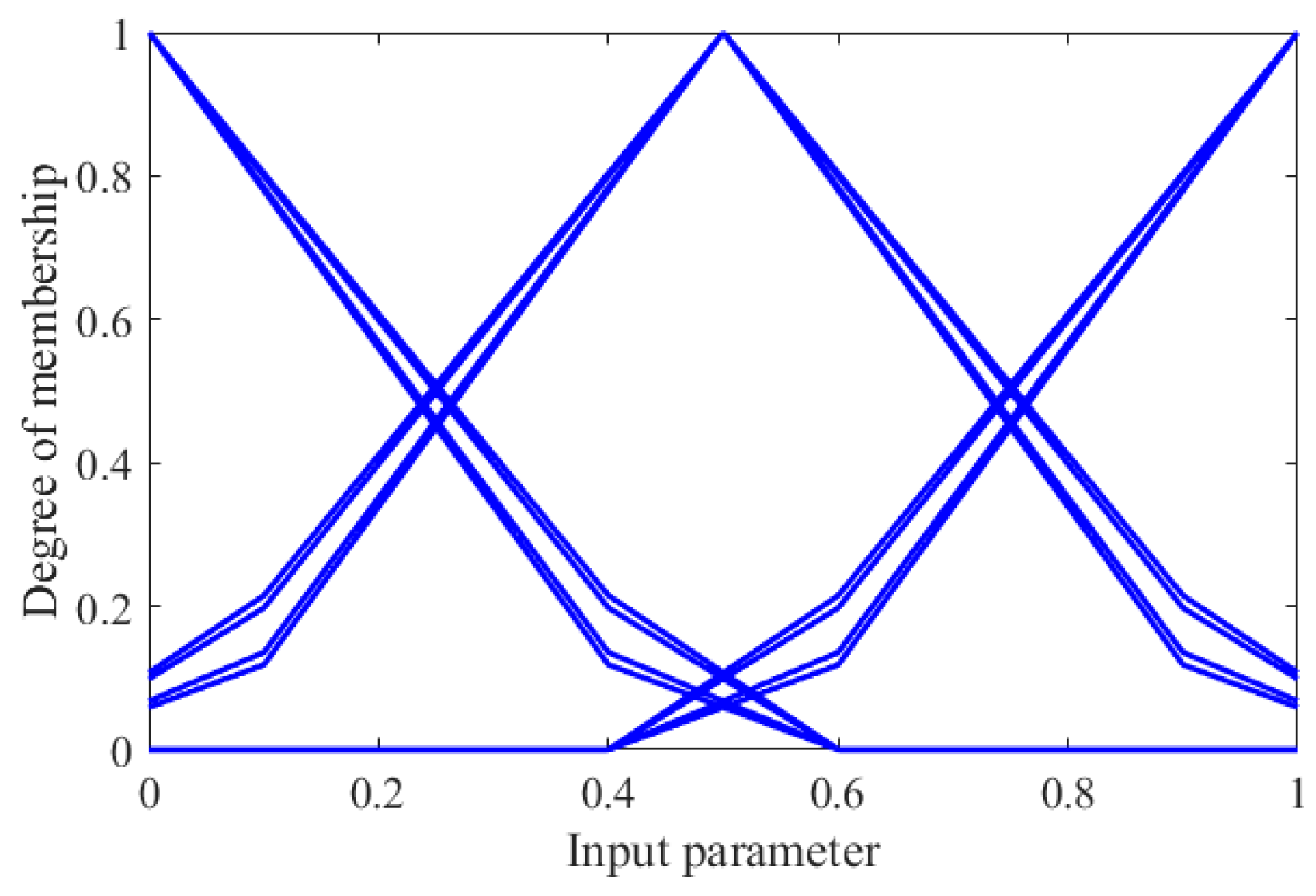
Algorithms 12 00017 g002
Figure 3. Input parameter membership functions.
Algorithms 12 00017 g003
Figure 4. Output parameter membership functions.
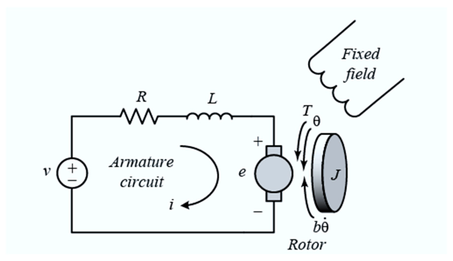
Algorithms 12 00017 g004
Figure 5. Motor position plant.
Algorithms 12 00017 g005
Figure 6. Structure of the motor position.
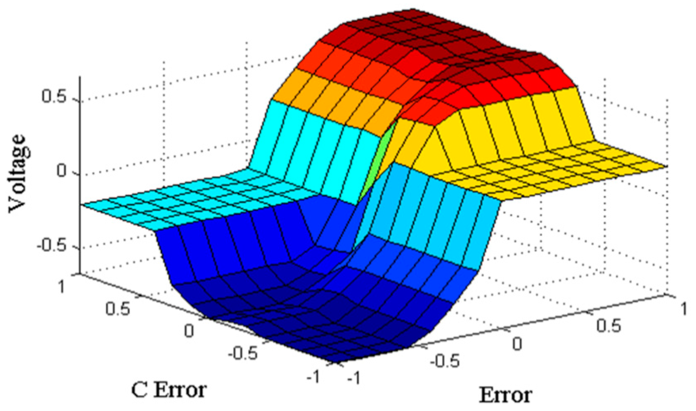
Algorithms 12 00017 g006
Figure 7. Surface of the fuzzy system.
Algorithms 12 00017 g007
Figure 8. Representation of the individuals for the T1 FIS.
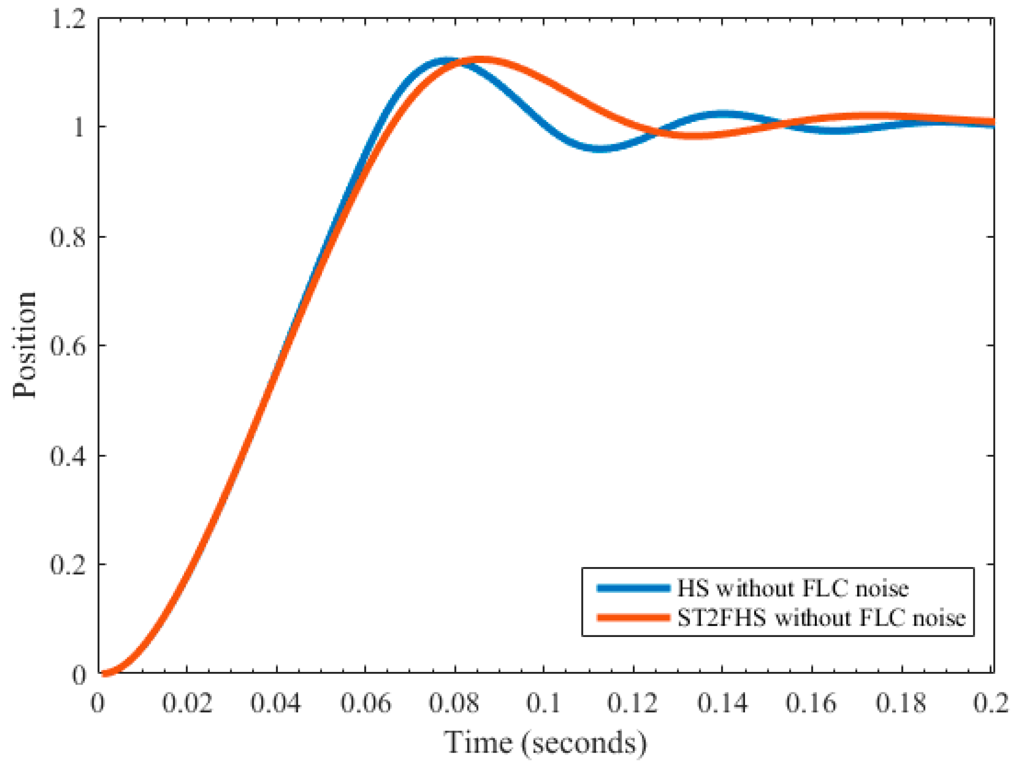
Algorithms 12 00017 g008
Figure 9. HS and ST2FHS without noise.
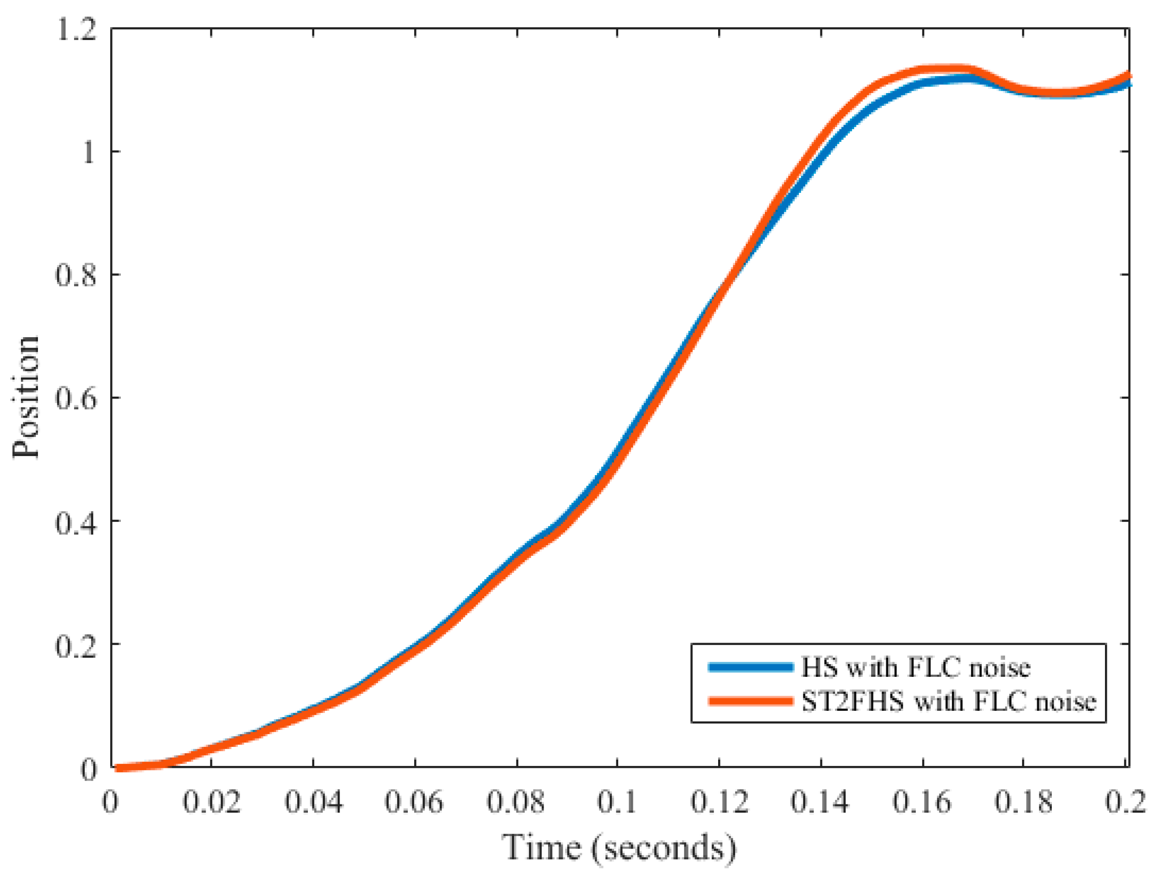
Algorithms 12 00017 g009
Figure 10. HS and ST2FHS with noise.
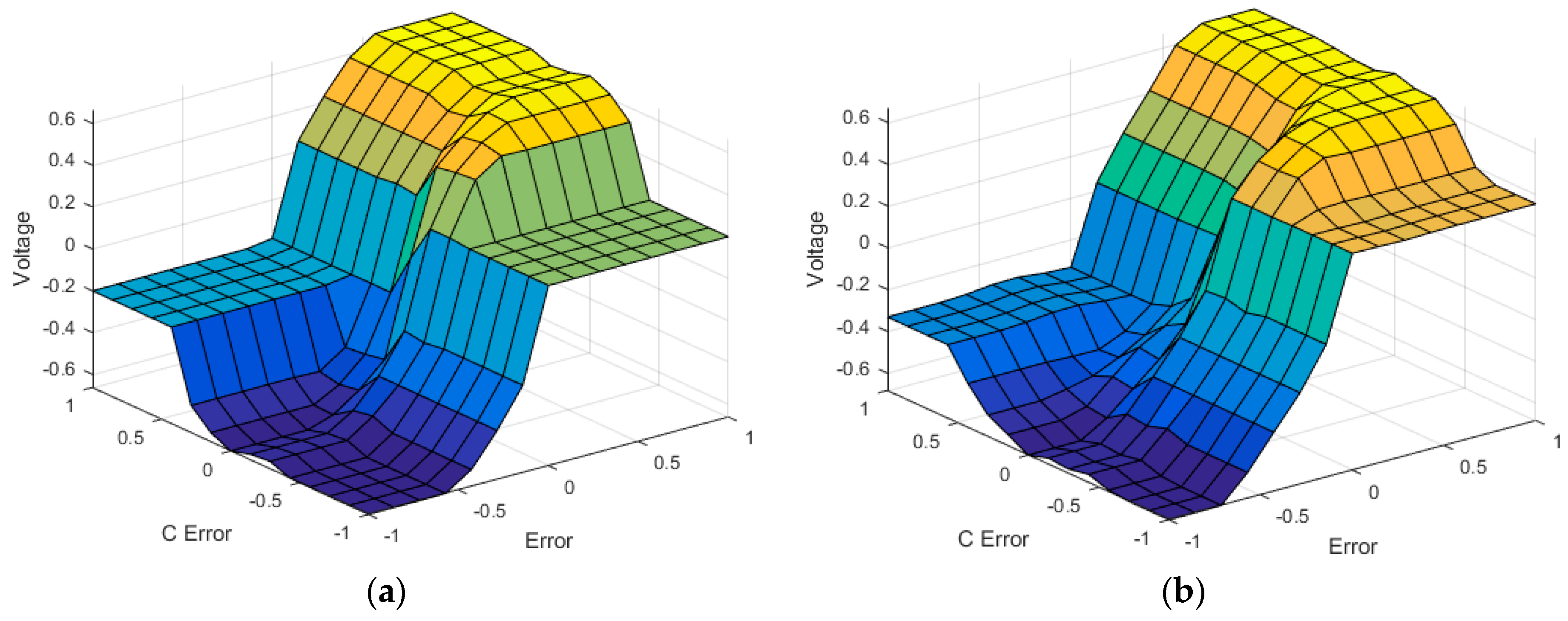
Algorithms 12 00017 g010
Figure 11. Comparison of the surface for each method for the motor position controller: (a) HS without noise algorithm; (b) ST2FHS without noise algorithm.
Algorithms 12 00017 g011
Figure 12. Comparison of the surface for each method for the motor position controller: (a) HS with noise algorithm; (b) ST2FHS with noise algorithm.
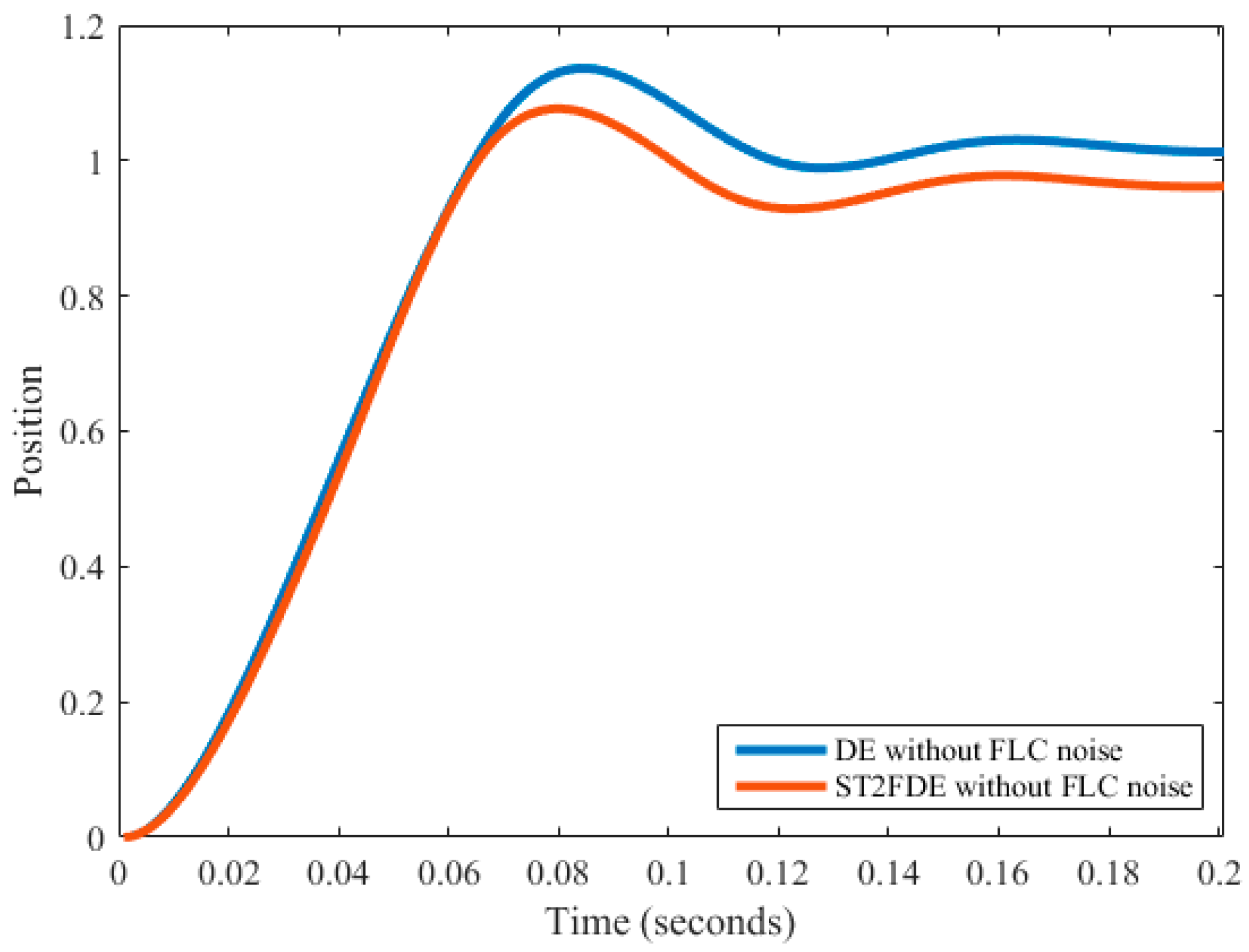
Algorithms 12 00017 g012
Figure 13. DE and ST2FDE without noise.
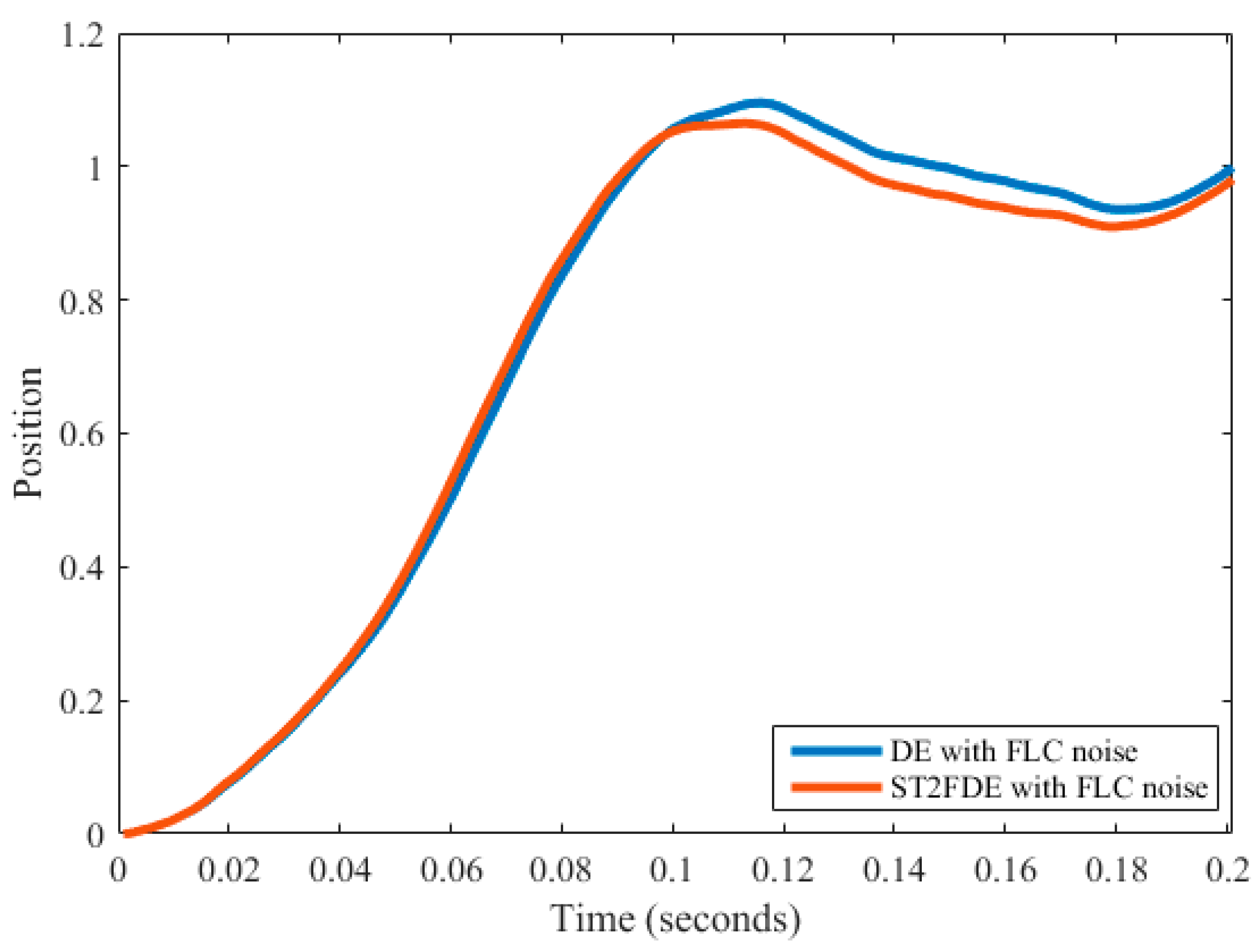
Algorithms 12 00017 g013
Figure 14. DE and ST2FDE with noise.
Algorithms 12 00017 g014
Figure 15. Comparison of the surface for each method for the motor position controller: (a) DE without noise algorithm; (b) ST2FDE without noise algorithm.
Algorithms 12 00017 g015
Figure 16. Comparison of the surface for each method for the motor position controller: (a) DE with noise algorithm; (b) ST2FDE with noise algorithm.
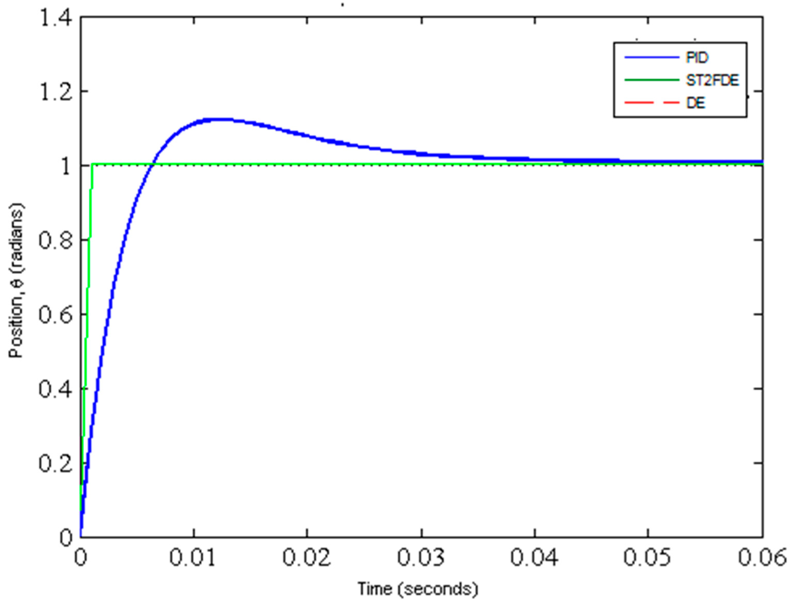
Algorithms 12 00017 g016
Figure 17. Structure of the PID (Proportional-Integral-Derivative) DC motor.
Algorithms 12 00017 g017
Figure 18. Best result obtained from the HS and ST2FHS methods.
Algorithms 12 00017 g018
Figure 19. Best results obtained from the DE and ST2FDE methods.
Algorithms 12 00017 g019
Table 1. Rules of the ST2FHS fuzzy system.
HMRLowMediumHigh
Iteration
LowLow
MediumMedium
HighHigh
Table 2. Rules of the ST2FDE fuzzy system.
FLowMediumHigh
Generation
LowLow
MediumMedium
HighHigh
Table 3. Benchmark mathematical functions.
FunctionSearch Domainf minEquation
Sum Squares[−10, 10]n0 f ( x ) = i = 1 n i x i 2
Trid[−100, 100]n−200 f ( x ) =   i = 1 n ( x i 1 ) 2 i = 2 n x i x i 1
Zakharov[−5, 10]n0 f ( x ) = i = 1 n x i 2 + ( i + 1 n 0.5 i x i ) 2 + ( i = 1 n 0.5 i x i ) 4
Ackley[−15, 30]n0 f ( x ) = a · e x p ( b × 1 n i = 1 n c o s ( c x i ) ) + a + e x p ( 1 )
Dixon & Price[−10, 10]n0 f ( x ) = ( x 1 1 ) 2 + i = 2 n ( 2 x i 2 x i 1 ) 2
Levy[−10, 10]n0 f ( x ) =   s i n 2 ( π w 1 ) +   i = 1 n 1 ( w i 1 ) 2   [ 1 + 10   s i n 2 ( π w i + 1 ) ] + ( w n 1 ) 2   [ 1 +   s i n 2   ( 2 π w n ) ] ,   w h e r e     w i = 1 +   x i 1 4 ,   f o r   a l l   i = 1 , . , n
Griewank[−600, 600]n0 f ( x ) = 1 400   i = 1 n X i 2 i = 1 n c o s ( x i i ) + 1
Powell[−4, 5]n0 f ( x ) = i = 1 n / 4 [ ( x 4 i 3 + 10 x 4 i 2 ) 2 + 5 ( x 4 i 1   x 4 i ) 2 + ( x 4 i 2   2 x 4 i 1 ) 4 + 10 ( x 4 i 3   x 4 i ) 4 ]
Power Sum[0, 10]n0 f ( x ) = i = 1 n [ ( j = 1 n x j i ) b i ] 2
Table 4. Results for the Sum Squares function.
Dimension10Z-Value50Z-Value
MethodHSST2FHS−16.78HSST2FHS−52.09
Best3.80 × 10−19.76 × 10−45.89 × 10−11.90 × 10⁻³
Worst1.26 × 103.50 × 10−31.02 × 103.00 × 10−3
Average7.07 × 10−12.02 × 10−38.10 × 10−12.28 × 10⁻³
SD2.30 × 10−15.19 × 10−48.48 × 10−22.67 × 10⁻⁴
Table 5. Results for the Zakharov function.
Dimension10Z-Value50Z-Value
MethodHSST2FHS−4.72HSST2FHS−2.41
Best7.34 × 10−114.00 × 10−132.04 × 10−43.12 × 10−4
Worst1.35 × 10−82.0869 × 10−96.97 × 10−39.47 × 10⁻⁴
Average3.27 × 10−93.63 × 10−101.42 × 10−36.37 × 10−4
SD3.33 × 10−94.73 × 10−101.76 × 10−31.49 × 10−4
Table 6. Results for the Dixon & Price function.
Dimension10Z-Value50Z-Value
MethodHSST2FHS−0.4HSST2FHS−7.67
Best7.30 × 10−31.39 × 10−32.56 × 101.53 × 10
Worst8.64 × 10−18.53 × 10−11.50 × 104.99 × 10
Average5.27 × 10−14.94 × 10−17.95 × 102.72 × 10
SD3.19 × 10−13.07 × 10−13.66 × 107.73 × 10−1
Table 7. Results for the Levy function.
Dimension10Z-Value50Z-Value
MethodHSST2FHS−0.23HSST2FHS−8.4
Best1.18 × 10−45.44 × 10−51.42 × 10−21.19 × 10⁻²
Worst3.39 × 10−43.25 × 10−41.98 × 10−21.63 × 10⁻²
Average2.25 × 10−41.90 × 10−41.66 × 10−21.41 × 10⁻²
SD5.64 × 10−51.92 × 10−41.33 × 10−31.01 × 10⁻³
Table 8. Results for the Griewank function.
Dimension10Z-Value50Z-Value
MethodHSST2FHS−0.29HSST2FHS0.22
Best4.57 × 10−21.55 × 10−13.65 × 10−29.75 × 10⁻¹
Worst8.49 × 10−12.94 × 10−12.15 × 101.02 × 10
Average2.28 × 10−12.25 × 10−11.00 × 101.00 × 10
SD4.57 × 10−23.65 × 10−21.59 × 10−21.02 × 10⁻²
Table 9. Results for the Power Sum function.
Dimension4Z-Value
MethodHSST2FHS−0.59
Best2.02 × 10−20.00 × 10
Worst2.47 × 100.00 × 10
Average2.23 × 101.71 × 10
SD4.48 × 101.84 × 10
Table 10. Results for the Trid function.
Dimension10Z-Value50Z-Value
MethodHSST2FHS−8.31HSST2FHS0.49
Best−1.23 × 10+2−1.90 × 10+2−3.49 × 10+3−2.98 × 10+3
Worst−1.19 × 10+2−1.80 × 10+2−1.33 × 10+3−1.39 × 10+3
Average−1.21 × 10+2−1.85 × 10+2−2.26 × 10+3−2.20 × 10+3
SD9.64 × 10−11.99 × 105.19 × 10+24.07 × 10+2
Table 11. Results for the Ackley function.
Dimension10Z-Value50Z-Value
MethodHSST2FHS−0.05HSST2FHS−0.6
Best5.66 × 10−56.68 × 10−55.14 × 10−25.75 × 10⁻²
Worst6.64 × 10−48.46 × 10−41.67 × 105.75 × 10−2
Average2.76 × 10−42.74 × 10−41.66 × 10−11.21 × 10⁻¹
SD1.50 × 10−41.65 × 10−43.48 × 10−12.08 × 10⁻¹
Table 12. Results for the Powell function.
Dimension10Z-Value50Z-Value
MethodHSST2FHS−7.03HSST2FHS−4.33
Best8.20 × 10−33.64 × 10−41.23 × 10−24.30 × 10⁻³
Worst1.70 × 10−12.40 × 10−34.32 × 10−11.76 × 10⁻²
Average5.88 × 10−21.37 × 10−38.18 × 10−21.11 × 10⁻²
SD4.47 × 10−25.17 × 10−48.90 × 10−23.43 × 10⁻³
Table 13. Results for the Sum Squares function.
Dimension10Z-Value50Z-Value
MethodDEST2FDE4.5513DEST2FDE−34.1921
Best9.48146 × 10−332.2026 × 10−313.7035072.7471 × 10−7
Worst3.80055 × 10−311.0944 × 10−296.5821058.4137 × 10−7
Average1.14269 × 10−311.7395 × 10−304.8514884.72 × 10−7
SD9.32651 × 10−321.9536 × 10−300.7771581.41 × 10−7
Table 14. Results for the Zakharov function.
Dimension10Z-Value50Z-Value
MethodDEST2FDE−10.5785DEST2FDE−37.0422
Best1.04 × 10−41.84 × 10−87.70 × 102.57 × 10−2
Worst7.64 × 10−41.87 × 10−71.43 × 10+21.06 × 10⁻¹
Average3.40 × 10−48.13 × 10−81.13 × 10+25.87 × 10⁻²
SD1.76 × 10−44.82 × 10−81.67 × 102.41 × 10−2
Table 15. Results for the Dixon & Price function.
Dimension10Z-Value50Z-Value
MethodDEST2FDE0.4408DEST2FDE−26.3743
Best1.77 × 10−12.54 × 10−11.60 × 10+26.68 × 10⁻¹
Worst6.67 × 10−16.67 × 10−14.01 × 10+27.55 × 10⁻¹
Average5.98 × 10−16.13 × 10−12.66 × 10+26.79 × 10⁻¹
SD1.49 × 10−11.12 × 10−15.51 × 101.81 × 10−2
Table 16. Results for the Levy function.
Dimension10Z-Value50Z-Value
MethodDEST2FDE0DEST2FDE−33.7726
Best1.50 × 10−321.50 × 10−323.20 × 104.74 × 10−7
Worst1.50 × 10−321.50 × 10−325.94 × 101.55 × 10−6
Average1.50 × 10−321.50 × 10−324.68 × 109.43 × 10−7
SD2.78 × 10−488.35 × 10−487.59 × 10−12.69 × 10−7
Table 17. Results for the Power Sum function.
Dimension4Z-Value
MethodDEST2FDE−1.6605
Best5.80 × 10−47.67 × 10⁻⁴
Worst2.21 × 10−22.26 × 10⁻²
Average9.15 × 10−36.65 × 10⁻³
SD6.18 × 10−35.46 × 10⁻³
Table 18. Results for the Trid function.
Dimension10Z-Value50Z-Value
MethodDEST2FDE0DEST2FDE−76.9252
Best−209−209−861.94−884.656
Worst−209−209−854.374−884.646
Average−209−209−858.184−884.651
SD001.8844780.002398
Table 19. Results for the Ackley function.
Dimension10Z-Value50Z-Value
MethodDEST2FDE−5.3864DEST2FDE−65.4158
Best4.44 × 10−158.88 × 10−161.82 × 101.60 × 10−4
Worst4.44 × 10−154.44 × 10−152.55 × 102.74 × 10−4
Average4.44 × 10−152.66 × 10−152.15 × 102.16 × 10−4
SD1.60 × 10−301.81 × 10−151.80 × 10−12.75 × 10−5
Table 20. Results for the Powell function.
Dimension10Z-Value50Z-Value
MethodDEST2FDE−9.5085DEST2FDE−36.7394
Best3.30 × 10−73.15 × 10−87.59 × 10+23.54 × 10⁻²
Worst5.76 × 10−63.54 × 10−71.32 × 10+31.13 × 10⁻¹
Average1.99 × 10−69.44 × 10−81.08 × 10+36.62 × 10⁻²
SD1.09 × 10−66.50 × 10−81.61 × 10+21.94 × 10⁻²
Table 21. Parameters of the motor position.
SymbolDefinitionValue
JMoment of inertia of the rotor3.2284 × 10−6 kg.m2
bMotor viscous friction constant3.5077 × 10−6 Nms
KeElectromotive force constant0.0274 V/rad/sec
KtMotor torque constant0.0274 Nm/Amp
RElectric resistance4 ohm
LElectric inductance2.75 × 10−6 H
Table 22. Type-1 membership functions.
Input Error
MFAbcd
NegV−1−1−0.50
CeroV−0.500.5-
PosV00.511
Input Error Change
ErrNeg−1−1−0.4−0.1
ErrNegM−0.4−0.20-
SinErr−0.0900.10-
ErrMaxM00.20.4-
ErrMax0.10.41-
Output Voltage
MDis−1−1−0.6−0.09
MDism−0.4−0.20-
Man−0.100.1-
Aumm00.20.4-
Aum0.090.611
Table 23. Fuzzy rules for the controller.
Voltage Error Change
ErrNegErrNeg_MSinErrErrMax_MErrMax
ErrorNegVDisDisDisDisDis_m
CeroVAum_mAum_mManDis_mDis_m
PosVAum_mAumAumAumAum
Table 24. Boundary T1 membership functions parameters of the vector.
Input 1Input 2Output
MF parametersFirst MF
a 0 = b 0 =   1
1   < c 0   < 0.5
d 0   = 0
First MF
a 0 = b 0 =   1
1   < c 0   < 0.4
d 0   = 0.1
First MF
a 0 = b 0 =   1
1   < c 0   < 0.6
d 0   = 0.09
Second MF
1   < a 1   < 0.1
b 1   = 0.2
0.1   < c 1   < 0
Second MF
1   < a 1   < 0.4
b 1   = 0.2
0.2   < c 1   < 0
Second MF
1   < a 1   < 0
b 1   = 0
0   < c 1   < 1
Third MF
0.09   < a 2   < 0
b 2   = 0
0   < c 2   < 0.10
Third MF
0.1   < a 2   < 0
b 2   = 0
0   < c 2   < 0.1
Fourth MF
0   < a 3   < 0.10
b 3   = 0.2
0.1   < c 3   < 1
Fourth MF
0   < a 3   < 0.1
b 3   = 0.2
0.09   < c 3   < 1
Third MF
a 2   = 0
0   < b 2   < 0.5
c 2 = d 2 =   1
Fifth MF
a 4   = 0.1
0.2   < b 4   < 0.4
c 4 = d 4 =   1
Fifth MF
a 4   = 0.09
0.2   < b 4   < 0.6
c 4 = d 4 =   1
Table 25. Results for the ST2FHS method.
MethodHS-FLC without NoiseST2FHS-FLC without NoiseHS-FLC with NoiseST2FHS-FLC FLC with Noise
Best7.86 × 10−37.32 × 10−34.22 × 10−21.95 × 10⁻²
Worst5.16 × 10−15.66 × 10−21.09 × 109.07 × 10−1
Average1.65 × 10−19.22 × 10−35.90 × 10−14.62 × 10⁻¹
SD1.37 × 10−13.45 × 10−33.07 × 10−12.83 × 10⁻¹
Table 26. Results for the ST2FDE method.
MethodDE-FLC without NoiseST2FDE-FLC without NoiseDE-FLC with NoiseST2FDE-FLC with Noise
Best7.34 × 10−34.35 × 10−32.24 × 10−25.89 × 10⁻⁴
Worst2.1 × 10−27.43 × 10−34.85 × 10−17.47 × 10⁻²
Average1.71 × 10−27.24 × 10−32.44 × 10−12.18 × 10⁻²
SD2.81 × 10−35.35 × 10−41.36 × 10−11.90 × 10⁻²
Table 27. Results for the statistical test of the DC motor.
Method μ 1 μ 2 Z-Value
ST2FHSFLC without noiseHS−6.23
FLC with noiseHS with noise−1.67
ST2FDEFLC without noiseDE−18.8799
FLC with noiseDE with noise−8.8627
Table 28. Results for the experiments with PID for the DC motor.
Method K p K i K d Best Settling Time
PID215000.150.0338
HS60012,00060.00029
DE9001800090.00020
ST2FHS90030,00090.00020
ST2FDE150030,000150.00012
Table 29. Results for the statistical test of the PID motor.
MethodST2FHSHSZ-Value
AverageStd.AverageSD−3.21
3.90 × 10−41.83 × 10−45.72 × 10−39.07 × 10−3
MethodST2FDEDE−2.53
AverageStd.AverageSD
3.03 × 10−42.15 × 10−44.22 × 10−38.46 × 10−3

