Article

Mixed Order Fractional Observers for Minimal Realizations of Linear Time-Invariant Systems

by
Manuel A. Duarte-Mermoud
1,2,*,
Javier A. Gallegos
1,
Norelys Aguila-Camacho
2,3 and
Rafael Castro-Linares
4
1
Department of Electrical Engineering, University of Chile, Av. Tupper, Santiago 2007, Chile
2
Advanced Mining Technology Center, University of Chile, Av. Tupper, Santiago 2007, Chile
3
Department of Electricity, Universidad Tenológica Metropolitana, Av. José Pedro Alessandri, Santiago 1242, Chile
4
Department of Electrical Engineering, CINVESTAV, Av. IPN, México DF 2508, Mexico
*
Author to whom correspondence should be addressed.
Algorithms 2018, 11(9), 136; https://doi.org/10.3390/a11090136
Submission received: 9 June 2018 / Revised: 5 September 2018 / Accepted: 7 September 2018 / Published: 9 September 2018

Abstract

:
Adaptive and non-adaptive minimal realization (MR) fractional order observers (FOO) for linear time-invariant systems (LTIS) of a possibly different derivation order (mixed order observers, MOO) are studied in this paper. Conditions on the convergence and robustness are provided using a general framework which allows observing systems defined with any type of fractional order derivative (FOD). A qualitative discussion is presented to show that the derivation orders of the observer structure and for the parameter adjustment are relevant degrees of freedom for performance optimization. A control problem is developed to illustrate the application of the proposed observers.

1. Introduction

We consider the observer design problem for a dynamic linear time-invariant system (LTIS) of a given differentiation order (DO). Assuming the knowledge at each instant of time of the pair of functions u , y : R 0 R , corresponding to the system input and output, respectively, the problem consists on finding an estimation of its internal variables (state or pseudo state) and of its parameters. To solve this problem, we propose a mixed order approach using minimal realizations, meaning that the observer and the system are defined in terms of the minimum number of parameters while the derivation orders used in the observer are arbitrarily chosen and possibly different from those of the system.
Non-mixed order observers (NMOO) have been proposed using Luenberger observers for integer order systems (IOS) and fractional order systems (FOS) [1,2,3,4,5,6]. Our contributions are summarized and commented in what follows.
  • In Section 2 we provide a mathematical framework for designing observer for LTIS, which includes systems defined by any generic fractional order derivative (GFOD) e.g., Caputo, Riemann–Liouville, etc. This is a subtle issue given the variety of fractional order derivatives (FOD) existent [7] and the fact that NMOO have been designed for specific type of derivatives [6,8,9,10,11,12]. In this framework, the concept of initial conditions (IC) is unambiguously defined and linear properties (superposition and separation) are easily obtained. Moreover, a minimal realization (MR) structure is chosen in the sense that the dimension of the internal variables is minimal and it is used the minimum number of parameters to describe the system, chosen to simplify the design. It yields a different structure from Luenberger observer.
  • In Section 3 and Section 4 convergence and robustness conditions are provided for non-adaptive and adaptive minimal realization observers (MRO) for commensurate systems. The conditions obtained meet those of the integer order observers (IOO) [4] when particularized to them, and constitutes a contribution in the non-mixed fractional order observers (FOO) literature for the adaptive case (cf. [8,9,13,14]), the latter being especially challenging, since currently there is not a fractional Lasalle theorem [15] available. The importance of this contribution is supported by the capability of fractional order systems (FOS) to model complex phenomena [10,16,17], whereby observers are needed since the internal variables are usually not accessible.
  • In Section 3 and Section 4 robust convergence conditions for adaptive and non-adaptive mixed-order observers (MOO) are stated, allowing in particular to design FOO for integer order systems (IOS) under the same assumptions than those of IOO. The difficulty is now to prove convergence and robustness for a system which is composed of subsystems with different DO. This novel idea makes possible (a) to dispose fractional calculus and their capabilities to model long memory effects [18] to observe real processes approximated by integer order (IO) linear systems, and (b) to have extra degrees of freedom (the derivation orders) to optimize criteria such as transient behavior, robustness, disturbance rejection, etc., which are relevant in current observer designs [19,20]. These advantages and some generalizations are qualitatively discussed in Section 3, Section 4 and Section 5 and a control application is developed in Section 6.
An alternative approach to robust non-mixed order observer (NMOO) is found in [21], where prior information on the uncertainty is required. In contrast, here only upper bounds are needed. Our observers are asymptotic; a nonasymptotic NMOO has been proposed in [12] for linear Riemann–Liouville systems and a specific class of uncertainties.

2. Linear Systems Preliminaries

Along this paper we consider a generic fractional order differential operator (GFODO) denoted as t = 0 D α or 0 D α , which satisfies the property that for any continuous function f, its Laplace transform holds that
L t = 0 D α f s = s α F s + F I C t = 0 , s , α , α > 0 ,
where F ( s ) denotes the Laplace transform (with lower limit t = 0 ) of the time function f ( t ) . F I C t = 0 , s , α is the Laplace transform of function f I C t = 0 , t , α and depends on the function f, the order α , ( t = 0 is the lower limit of the Laplace Transform) and the type of fractional derivative. Examples are Caputo (e.g., F I C t = 0 , s , α = f 0 s α 1 for α < 1 ), Riemann–Liouville ( F I C t = 0 , s , α = { D α 1 f } 0 for α < 1 ), Grunwald-Letnikov ( F I C t = 0 , s , α = 0 for α < 1 ) and Miller-Ross fractional derivative ([16], Section 2.8) among others. For the fractional integral, there is a commonly chosen definition, which in Laplace domain takes the form,
L t = 0 I α f s = s α F s α > 0 ,
and in time domain, it is given by
0 I α f ( t ) : = 1 Γ ( α ) 0 t ( t τ ) α 1 f ( τ ) d τ .
where Γ ( · ) is the Gamma function [16].
Fractional order linear systems (FOLS) can be represented in Laplace domain by taking Laplace transform to the input/output pair ( u ( t ) , y ( t ) ) to obtain ( U s , Y s ) : = L { u , y } s . Assuming null IC conditions, a linear relationship is obtained expressed in terms of the complex variable s of the form Y ( s ) = H ( s , U ( s ) ) = H ( s ) U ( s ) , where H is called the Transfer Function (TF) (Transfer Matrix in the vector case). In particular, we are interested in TF of the type
H s = i = 0 m b i s β i i = 0 n a i s α i ,
where α 0 < < α n ; β 0 < < β m ; a 0 , a n and b 0 , , b n are numbers in R . It follows that
Y ( s ) = b n s β n + + b 0 a n s α n + + a 0 U ( s ) + i = 1 m b i U I C i 0 , s , β i i = 1 n a i Y I C i 0 , s , α i a n s α n + + a 0 ,
where L [ a i D α i y ] = a i s α i Y ( s ) + a i Y I C i 0 , s , α i and L [ b i D β i u ] = b i s β i U ( s ) + b i U I C i ( 0 , s , β i ) . In view of (5), the terms Y, U in time domain can be called initial conditions (IC), since they uniquely define the output y for each input u (see discussion in Section 5.4). More precisely, the IC must be all what is undetermined in U, Y. For instance, if Y = s α 1 { y 0 } , the IC must be y ( 0 ) .This procedure can be easily generalized for the vector case. From this, we obtain some elementary properties for generic fractional order linear systems (GFOLS):
  • P1: The superposition of responses to a linear combination of inputs holds when the IC are null.
  • P2: The solution to (5) is the sum of a zero state solution (first term of (5)) plus a zero input solution (second term of (5)).
Since we are interested in observing internal variables (state or pseudo state variables), we look for a suited mathematical model of internal variables for (4). In the commensurate case α i = l i α and β i = m i β for some integers numbers l i , m i and making the identification s α = s , some standard results for IOLS also hold for FOLS.
In particular, we can consider a completely controllable and observable system (i.e., (4) cannot be further simplified), for which we choose, without loss of generality (since, by applying Laplace transform, the resulting system will be input-output equivalent to (4)), the following canonical representation for x R n and y , u R and the matrices A , b , c having suited dimensions:
0 D α x = A x + b u y = c T x x I C t = 0 , t , α = ψ 0 , ( I C )
where α > 0 , x I C t = 0 , t , α is the IC (a generalized time function or the Laplace transform inverse of X I C t = 0 , s , α obtained according to (1)) and
A = a 1 1 0 0 0 a n 1 0 0 1 a n 0 0 , b = b 1 b n , c = 1 0 0 .
Note that we use the minimal number of parameters necessary to describe the system and, since the system is completely controllable and observable, the minimal dimension for the internal variables corresponding to the number of components of x. Any other minimal representation x of the system is related to (6) through a linear transformation x = T x with T nonsingular.
Consider the following matrices
F = f 1 1 0 0 0 f n 1 0 0 1 f n 0 0 , g = g 1 g n ,
where the elements of F are chosen such that x = 0 is globally attractive for the system D α x = F x , i.e., any of its solutions converges to zero as time goes to infinity. We can write A x = ( F + A F ) x = F x + ( A F ) x and, choosing g i = a i f i together with the structures of A and F, it follows that ( A F ) x = g c T x = g y . Thus, we can write A x = F x + g y and therefore system (6) can be re-expressed as
0 D α x = F x + g y + b u y = c T x x I C t = 0 , t , α = ψ 0
By linearity, the solution to (7) can be expressed as the sum of the response to a null input with nonzero IC (zero input response) plus the response when ψ 0 0 (null IC) to a nonzero input (zero state response). The former is just the solution to D α x = F x when X t = 0 , t , α = ψ 0 ; we denote it by ξ t ; x 0 , α . For the latter, we observe that superposition can be used since the IC are null. To this aim, we define for i = 1 , , n the following system
0 D α η i = F η i + e i y 0 D α η i + n = F η i + n + e i u η I C i ( t = 0 , t , α ) η I C i + n ( t = 0 , t , α ) 0 ,
where e i is the i - element of the canonical base of R n . Hence, the response to g y + b u = i = 1 n g i e i y + h i e i u is i = 1 n g i η i + h i η i + 1 . Therefore, for t > 0
x ( t ) = ξ ( t ; ψ 0 , F , α ) + [ η 1 η 2 n ] ( t ) p ,
where p = ( g 1 , , g n , b 1 , , b n ) T is a vector of parameters.
To end this section, we recall that for Caputo or Riemann–Liouville FOS, if | a r g s p e c F | > α π 2 , then x = 0 is globally attractive for the system 0 D α x = F x , where s p e c F is the set of eigenvalues of F [11]. It follows that if F is such that x = 0 is globally attractive for 0 D α x = F x , then x = 0 it is globally attractive for 0 D β x = F x , where 0 < β < α .
For other FOS, the condition | a r g s p e c F | > α π 2 assures BIBO stability, that is that the transfer function of 0 D α x = F x , H α s = s α I F 1 is Lebesgue measurable in time domain, i.e., 0 | | H α t | | d t < [22]. To assure the attractiveness of x = 0 , the following condition on the chosen derivative (specifically, on the IC term X I C t = 0 , s , α ), must hold in addition
lim s 0 s s α I F 1 X I C t = 0 , s , α = 0 .

3. Non-Adaptive Mixed Order Observer (NAMOO)

Based on minimal representations, Luenberger observers [1] can be generalized for fractional order systems following the results in [3]. Consider system (6) with A , b , c known and not necessarily in any canonical form. Define the estimate x ^ of the internal variable x by
0 D α x ^ = A x ^ + b u + F y y ^ y ^ = c T x ^ x ^ t = 0 , t , α = ψ ^ 0
Note the FO is the same for the system (6) and the observer (11). It follows that e : = x x ^ satisfies D α e = A F c T e . Since it is a minimal representation, matrix F can be chosen such that the matrix ( A F c T ) has arbitrary eigenvalues. Therefore, we get asymptotically e 0 as t .
We will build an alternative observer whose FO is not equal to the order of the original system. Moreover, it is minimal not only in the internal variable dimension but also in the use of the minimal numbers of parameters to describe the system, all the rest being freely chosen to simplify the design.
Consider the state observer for system (6) given by
0 D β x ^ = F x ^ + y ˜ + u ˜ y ^ = c T x ^ x ^ t = 0 , t , β = ψ ^ 0
where u ˜ , y ˜ are filtered versions of u , y given, in Laplace domain, by
Y ˜ = s β I F s α I F 1 g Y U ˜ = s β I F s α I F 1 b U
with null IC for u ˜ , y ˜ . Consider system D β x = F x with F chosen such that x = 0 is asymptotically stable or more generally, globally attractive, then we have the following result stated in the next Theorem.
Theorem 1.
Let us consider system defined in (6). Then we can state that system (12) is an asymptotic observer with speed of convergence regulated by the eigenvalues of F. Besides, the observer is robust with respect to external perturbations, meaning that:
(a) 
If u , y have additive bounded uncertainties, i.e., u t + Δ u t and y t + Δ y t , the estimates of internal variables and the output error remain bounded, having also high frequency rejection.
(b) 
If parameter vector p (i.e., the elements of A and b) is in fact p + Δ p , where parameter disturbances n Δ p , u and y are bounded functions, then x x ^ and y y ^ remain bounded.
Proof. 
The solution of (12) is given by
x ^ = ξ t ; ψ ^ 0 , F , β + η 1 η 2 n p
where we have used that the solution when ψ ^ 0 0 is given, in Laplace domain, by s β I F 1 s β I F s α I F 1 g y + b u = s α I F 1 g y + b u , the same solution for (7) when ψ 0 0 .
From (9) to (14), we obtain that, x ^ t x t = ξ t ; ψ ^ 0 , F , β ξ t ; ψ 0 , F , α . Hence, lim t x ^ t x t = 0 and lim t y ^ t y t = lim t c T x ^ t c T x t = 0 accordingly to the choice of F.
If the input is now u t + Δ u t and the output is y t + Δ y t , then (14) is modified to
x ^ t = ξ t ; ψ ^ 0 , F , β + η 1 η 2 n t p + Δ t
where Δ ( t ) is the time domain expression of s α I F 1 g Δ y + b Δ u . Since s α I F 1 is a BIBO stable filter according to the choice of F and Δ u , y are bounded, we conclude that Δ is a bounded function. It follows that x ^ t x t = ξ t ; x 0 , F , β ξ t ; x 0 , F , β + Δ t , and therefore y ^ y , are bounded.
If the parameters are changed to p + Δ p , then x ^ t x t = ξ t ; ψ ^ 0 , F , β ξ t ; ψ 0 , F , β + η 1 η n Δ p . Since u , y were assumed bounded, and since F was chosen such that system (8) is BIBO stable, we conclude that x ^ t x t and therefore y ^ y , are bounded. ☐
Remark 1.
(i) 
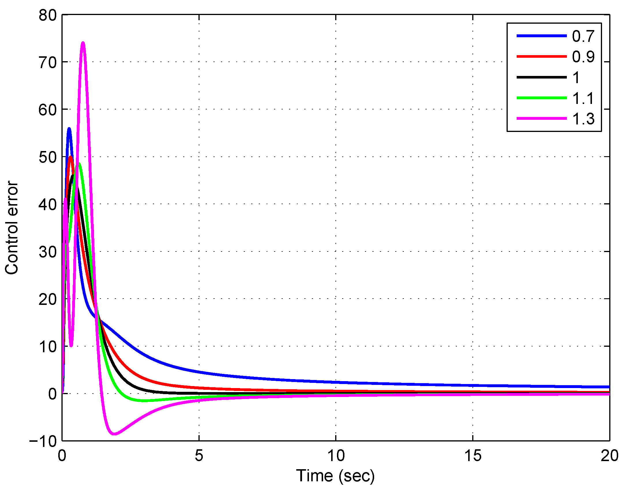
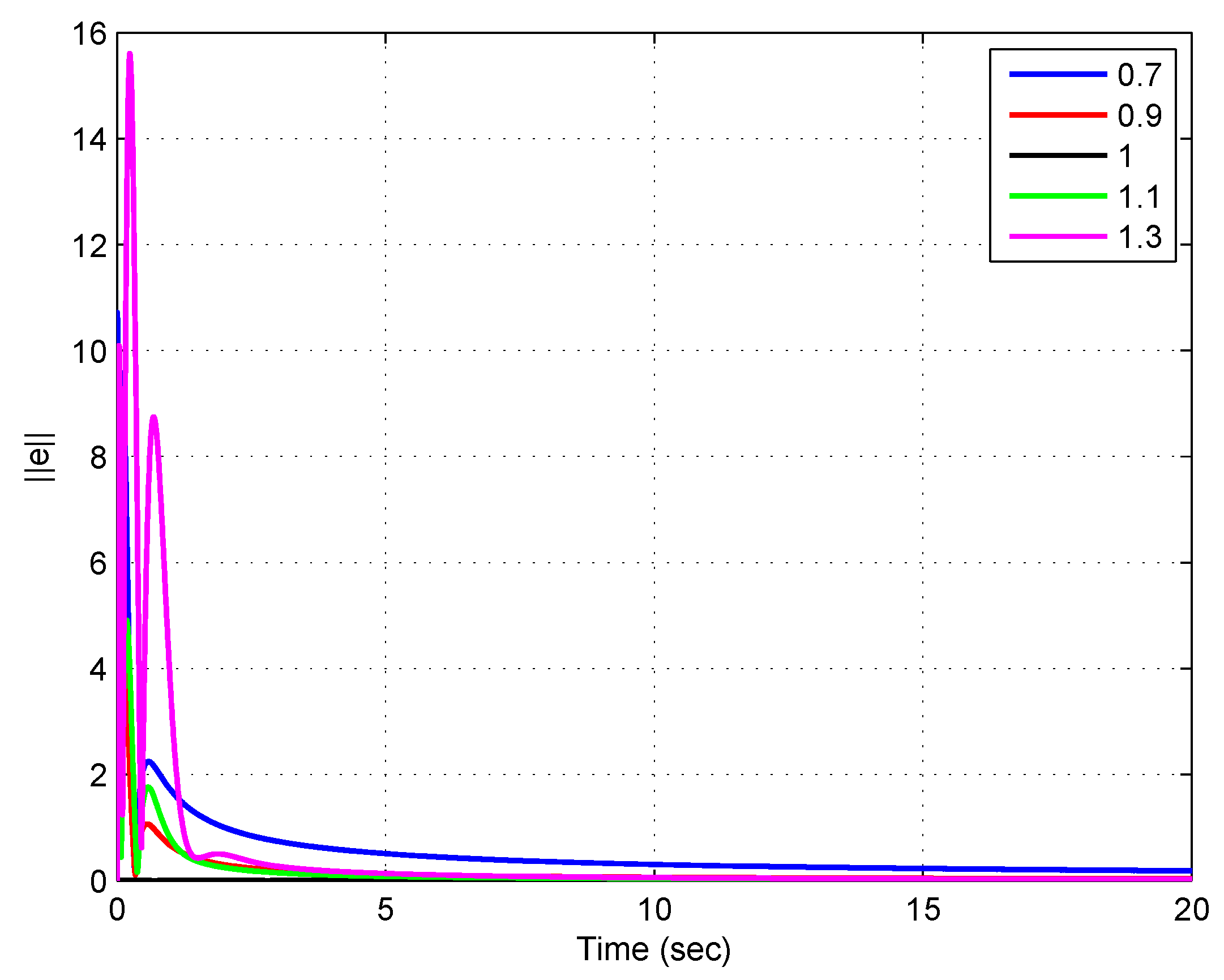
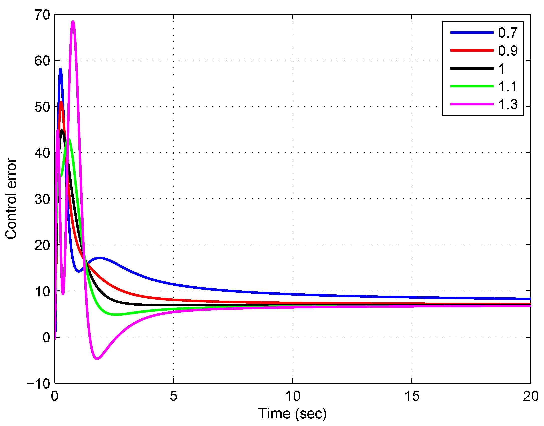
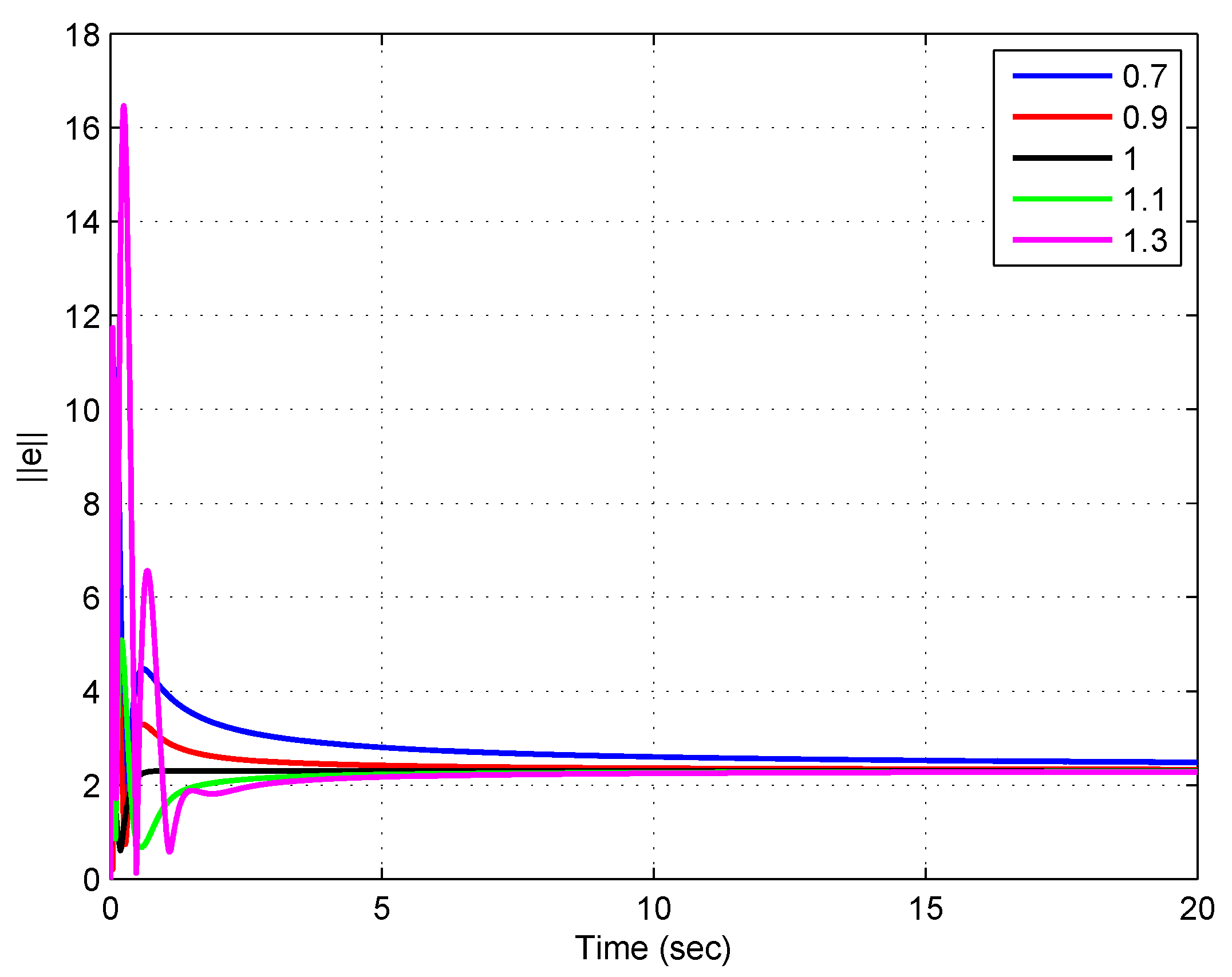
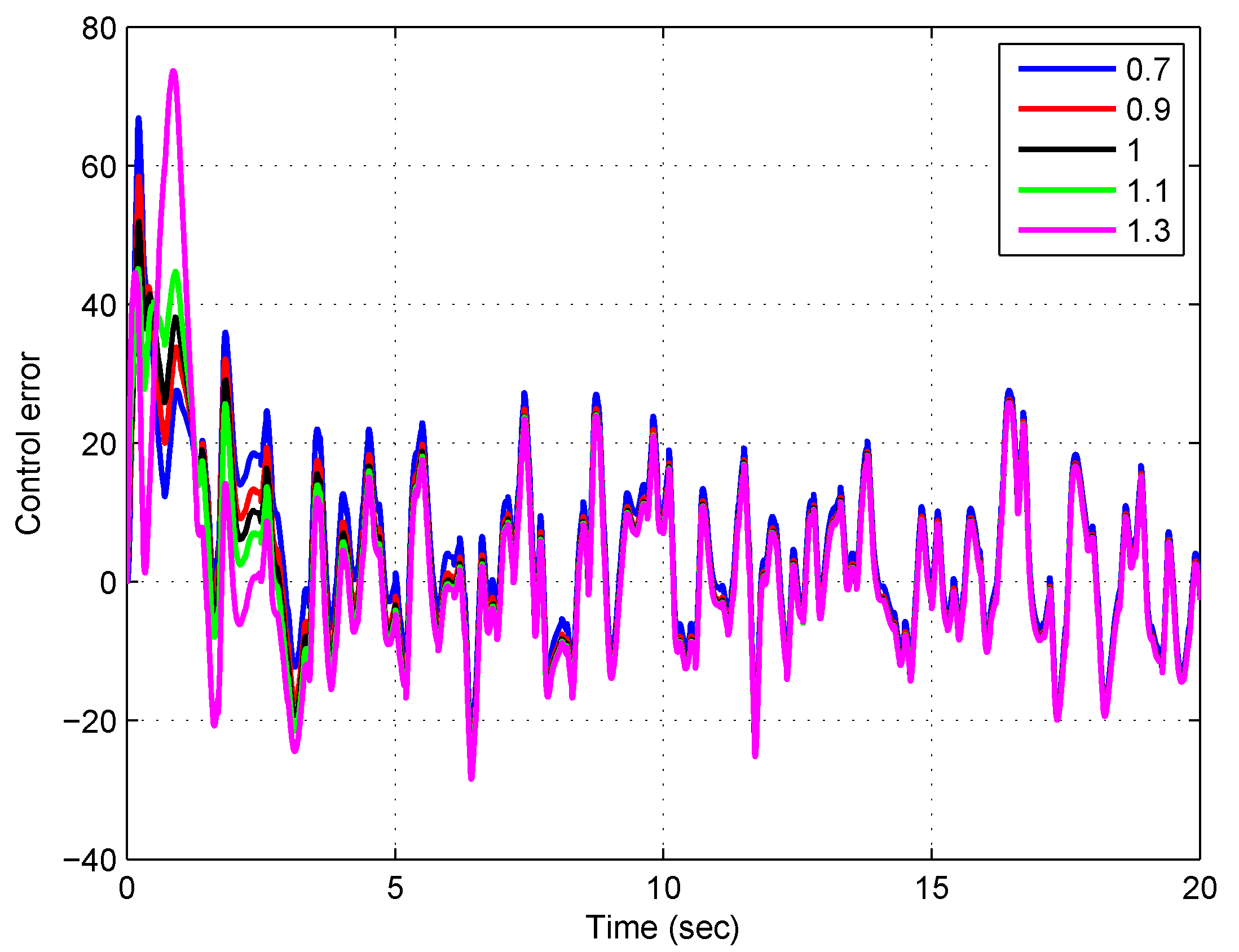
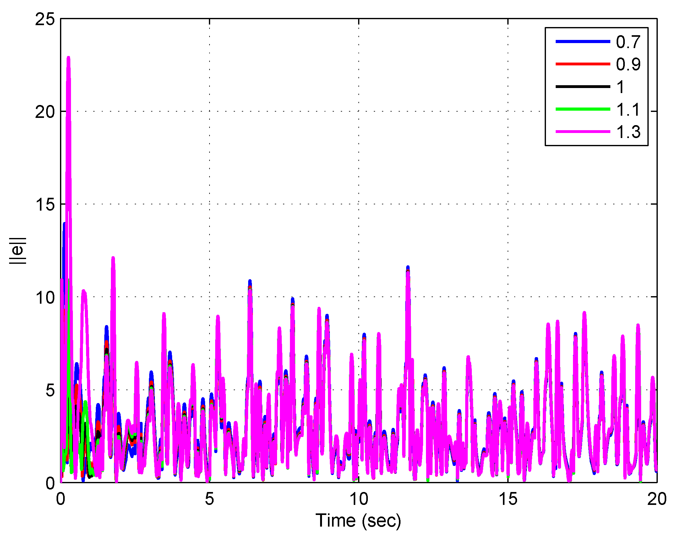
A benefit of the MO approach to design observers is that the transient behavior of the estimate x ^ can be regulated by the choice of the FO β. A NMFOO where β = α —like the Luenberger observer (11)—can only regulate the speed of convergence through the choice of F.
(ii) 
Unlike Luenberger observer (11), there is no need of an output error feedback term F y ^ y . Since this term is essential in the stability proof of the Luenberger observer, the introduction of this term in our designs can give some freedom to further improvements.

4. Adaptive Mixed Order Observer (AMOO)

In this section we consider that vector p (i.e., the elements of A and b) in system (7) is unknown. Thus, instead of p we will use an estimation of it, p ^ = p ^ t , for the proposed observer scheme in Section 3. Using expression (14), we write
x ^ t = ξ t ; ψ ^ 0 , F , β + η 1 η 2 n t p ^ t ,
where η i are calculated using only the input and output information as in (7) or (8), and c is known from the canonical representation chosen for the system (6). We will use the information vector defined by W : = η 1 η 2 n c and it will be assumed the Caputo derivative along this section.
We will state a previous result to assure the stability of the AMOO, given in the following Lemma.
Lemma 1.
The solutions to the Caputo system 0 D α x = A x , with x 0 R n , have bounded quadratic γ - fractional integral, if 0 < γ 2 α and | a r g s p e c A | > α π 2 .
Proof. 
Let ξ be a solution for x 0 = x 0 . Since the solution is continuous at 0 , T for every T > 0 [16], provided that u is continuous, only the behavior of ξ 2 as t is decisive to determine if its fractional integral is bounded.
In Laplace domain, we can write ξ ^ s = s α 1 ( s α A ) 1 x 0 = : s α 1 H α s . We have that H α in time domain is an L 1 function in each component (see e.g., [23], or [24]). Therefore, as t , ξ has a behavior in Laplace domain given by lim s 0 s α 1 H α s . Since the relative degree of each component of H α is non-negative, this limit is s α 1 x 0 which in time domain is proportional to t α x 0 . Therefore, the condition γ 2 α to have bounded fractional integral of ξ 2 is thus easily obtained. ☐
Theorem 2.
Consider the observer (16) for a stable system (6) such that the parameter estimation is performed as
t 0 D γ p ^ = κ y ^ y W ,
where t 0 0 , κ > 0 , γ 2 min { α , β } or γ 2 α and x ^ 0 = 0 . Then,
(i) 
All the variables of the system remain bounded, y ^ y has bounded γ-integral and its R M S value converges to zero. These claims remain true if a bounded additive perturbation of quadratic bounded γ - integral is added on the input and/or output of the system (6).
(ii) 
If the spectral measure of u is not concentrated on k < 2 n points, then p ^ converges to the true parameters of the plant p and x ^ converges to x as t .
Proof. 
(i)
From (9) to (16), it follows that
x ^ t x t = ξ t ; ψ ^ 0 , F , β ξ t ; ψ 0 , F , α η 1 η 2 n t p ^ t p .
Hence,
c T x ^ t x t = c T ξ t ; ψ ^ 0 , F , β ξ t ; ψ 0 , F , α + c T η 1 η 2 n t p ^ t p e t : = y ^ t y t = ν t + W T t p ˜ t
where e is the output error and p ˜ = p ^ t p is the parameter error. It follows that ν 2 : = c T ξ t ; ψ ^ 0 , F , β ξ t ; ψ 0 , F , α 2 has bounded γ - integral. Indeed, from the hypothesis on γ , the choice of F and Lemma 1, c T ξ t ; x ^ 0 , F , β and c T ξ t ; x 0 , F , α have bounded quadratic γ - integral. By recalling that | | x + y | | 2 2 | | x | | 2 + 2 | | y | | 2 , we obtain that ν has bounded quadratic γ - integral by (say) a constant number C.
Without loss of generality, we assume κ = 1 (otherwise, we always can redefine W as κ W ). Let V : = p ˜ T p ˜ + C 1 / 2 I γ ν 2 . Note that V is non-negative, since ν has bounded quadratic γ - integral. By ([25], Theorem 3) and continuity of the solutions, t 0 D γ p ˜ T p ˜ t 2 p ˜ T t t 0 D γ p ˜ t [26,27]. Using that t 0 D γ p ˜ = t 0 D γ p ^ , since p is constant, together with (17) and (19), we obtain
D γ V 2 p ˜ T W 2 2 p ˜ T W ν 1 / 2 ν 2 = 2 p ˜ T W + 1 / 2 ν 2 0 .
By γ - integration of (20), we obtain V t V 0 . That is, p ˜ T p ˜ + C 1 / 2 I γ ν 2 is bounded. Since C > 1 / 2 I γ , it follows that p ^ is bounded. Using the BIBO stability property of system (8) due to the choice of F, it follows that W is bounded whenever y , u are bounded. Then, e is bounded. By γ - integration of (20), we also conclude that e 2 = p ˜ T W + 1 / 2 ν 2 has bounded γ -integral. Thus, e R M S converges to zero ([28], Proposition 1).
Using expression (15) and redefining ν , we have also proved that if a bounded perturbation Δ with bounded quadratic γ - fractional integral, is added to the model input and/or output, all the above claims remain true.
(ii)
If the spectral measure of u is not concentrated on k < 2 n points, W = η 1 is a persistently exciting (PE) function ([28], Property 11). Using this and the fact that ν converges to zero, it follows that p ˜ converges to zero ([24], Section 3) i.e., p ^ converges to p. Since u , y are bounded, η i is bounded for i = 1 , , 2 n . Therefore, using (18), x x ^ converges to zero.
For additive bounded perturbations on the parameters, we can redefine ν which is now just a bounded function. According to ([24], Section 3), p ^ , e remains bounded, when W is a PE function. Moreover, if the perturbation vanishes as t goes to , then p ˜ , e converges to zero. ☐
Remark 2.
A benefit of the adaptive scheme (17) when γ < 1 is shown by the following reasoning. From the facts that (a) if ν 2 has bounded γ 1 - integral, then it has bounded γ 2 - integral for any 0 < γ 2 γ 1 (the proof is by contradiction and using I γ 1 ν 2 = I γ 1 γ 2 I γ 2 ν 2 ) and that (b) t γ has bounded γ - integral but unbounded integer integral when γ < 1 , it follows that the set of non-destabilizing perturbations for the adaptive scheme is strictly enlarged for γ < 1 . The following heuristic rule can be stated as the lesser the value of γ the more robust is the response.

5. Discussion

In this section we examine some assumptions made for the proposed observers and discuss some ways to generalize it.

5.1. Non-Conmensurate Systems

We have assumed that both observer and system were commensurate. Although non-commensurate rational orders systems can be turned into a commensurate system in a common order, if this mechanism is used the precedent results yield a non-minimal observer. A Luenberger-like observer can be used but only for the NMOFO case. A particular case can be analyzed for MOFO as shown below.
Suppose that the non-commensurate system can be expressed by (6) where α is to be seen as a vector, so that D α x D α 1 x 1 , , D α n x n T . Let H α = H α s be the transfer matrix from X ( s ) to the input g Y ( s ) + b U ( s ) . Then, this system can be observed with a commensurate observer (12) with (13) redefined as
Y ˜ = s β I F H α g Y U ˜ = s β I F H α b U
provided that F is such that the origin x = 0 of both, 0 D α x = F x and 0 D β x = F x , are globally attractive.

5.2. Adaptive Observer for Unstable Plants or Non-Caputo Systems

If the information vector W is not assumed to be bounded, the adaptive law can be modified including a normalizing factor defined as
t 0 D γ p ^ = κ y ^ y W 1 + W T W .
Along the same lines of the proof of Theorem 2, it can be shown that the properties of the error in Theorem 2(i) hold for e 1 + W T W instead of e and the convergence properties in Theorem 2(ii) hold if W 1 + W T W is of PE type.
When α 1 , a MO adaptive adjustment with γ = 1 , is obtained using
D p ^ = Γ W y ^ y D Γ = Γ W W T Γ Γ t i = I
where t i + 1 : = t i + δ i and δ i : = a r g m i n Δ t i t i + Δ w ^ w ^ T ϵ I . By assumptions and arguments in the proof of Theorem 2(ii), W is a PE function. By applying ([29], Lemma A3), it follows that p ^ exponentially converges to p. Since η i can diverge in order t α , it follows that x ^ converges x.
The use of Caputo derivative along Section 4 has two main reasons. The first is that in the proof of Theorem 2, it is needed that the derivative of a constant number must be zero. Any other derivative with this property can be used. The second is also related to the proof of Theorem 2 and the choice of Caputo derivative, since an additive term associated with the IC, must be controlled. Any system satisfying a similar statement of Lemma 1 can be used.

5.3. A Non-Local Observer for a Local System?

When α = 1 and β 1 , we are observing a local system with a non-local observer. Apparently this looks like an unnecessary waste of computational resources. However, and besides Remarks 1 and 2, there is a practical consideration that can be argued in favor of a MO strategy.
Linear models are at best good approximations of real processes, which are generally infinite dimensional and nonlinear with long or short memory properties. Moreover, noisy measurements are also present in real processes. These aspects are commonly represented by an additive term ν = ν t representing unmodeled dynamics. Thus, the system (6) (or (7)) is rather
0 D α x = F x + g y + b u + ν y = c T x .
Seeing ν as an stochastic process, the locality of the system is assured only if ν is a Markov process. For a non-Markov process, the observed system is non-local and it can be expected that a local observer yields poorer results than using a nonlocal observer.

5.4. Unknown Initial Time

When α 1 , the schemes proposed in Section 3 and Section 4, implicitly assumes that the initial time of the observed system is known and the same for the observer system. This is an unrealistic assumption which is found in all the revised papers (see e.g., [3]), with the exception of those that use diffusive fractional systems. This consideration does not apply to the adaptive law (17) which can be applied at any instant without changing Theorem 2.
We show that the framework of Section 2 allows to deal with this case in a consistent way. Let t 0 < 0 the unknown initial time of the observed system and t = 0 the initial time of the observing process. Consider the system given by
t 0 D α x = A x + B u = : A ¯ ( x , u ) ,
where the derivative is generic in the sense of (1). In particular, by applying Laplace transform for the time variable t : = t t 0 , it holds that [ t 0 D α x ] ( s ) = X ^ ( t 0 , s , α ) + s α x ^ . Applying α - fractional integral from t = 0 , we obtain
s α [ t 0 D α x ] ( s ) = s α X ^ ( t 0 , s , α ) + x ^ ( s ) = : ψ ^ 0 ( t 0 , s , α ) + x ^ .
Hence, the α - fractional integral of (22) yields in the time variable t
x ( t ) = ψ 0 ( t 0 , t , α ) + 1 Γ ( α ) t 0 0 ( t τ ) α 1 A ¯ d τ + 1 Γ ( α ) 0 t ( t τ ) α 1 A ¯ d τ = : ψ 1 ( 0 , t , α ) + 1 Γ ( α ) 0 t ( t τ ) α 1 A ¯ d τ
Applying Laplace Transform for the time variable t, we obtain
x ( s ) = ψ ^ 1 ( 0 , s , α ) + s α [ A x ^ + B u ^ ] s α x = s α ψ ^ 1 ( 0 , s , α ) + A x ^ + B u ^ = : ψ ^ ( 0 , s , α ) + A x ^ + B u ^ .
Therefore, by defining [ D ¯ α x ] ( s ) : = s α x ψ ^ ( 0 , s , α ) , we have that the system D ¯ α x = A x + B u is equivalent to (22) for t 0 , in the sense that both have the same solution for t 0 . In particular, the term ψ ( 0 , t , α ) can be identified as the IC term. Note that, in general 0 D ¯ α 0 D α , since both have different IC terms. Theorems 1 and 2 still hold, but the care must be put in finding F verifying Equation (10) of Section 2.
Another important fact is that if the observed system started at t = t 0 from rest, meaning that any kind of IC becomes identically zero, i.e., ψ 0 0 for any chosen derivative, then the FOS is unequivocally defined, meaning that there is not ambiguity in the choice of the derivative, since any of them yields the same IC term ( ψ ) for any t t 0 . Only in this way, we can talk of a FOS, in the sense of [30]. On the other hand, if the system started at non-null IC, it has sense talk of a Caputo or RL or any other generic FOS.
We have the following specifications to the above procedure, for a Caputo FOS.
ψ 0 ( t 0 , s , α ) = s α s α 1 x ( t 0 ) = s 1 x ( t 0 ) ψ 0 ( t 0 , t , α ) = x ( t 0 ) , t > t 0 , ψ 1 ( 0 , t , α ) = x ( t 0 ) + 1 Γ ( α ) t 0 0 ( t τ ) α 1 [ A x + B u ] d τ ψ ( 0 , s , α ) = s α 1 x ( t 0 ) + s α L { 1 Γ ( α ) t 0 0 ( t τ ) α 1 [ A x + B u ] d τ } ( s ) .
In particular, the resulting D ¯ α is not a Caputo one. This is what some authors refer as that Caputo derivative does not take account of the past [31]. To the best of our knowledge, it seems there is no a fractional derivative operator yielding D ¯ α = D α (the diffusive approach is not realizing a known fractional derivative operator).
Finally, when taking the same F as the last paragraph of Section 2, and using expression (10), we obtain for any t 0
lim s 0 s s α I F 1 { s α 1 e ( t 0 ) + s α L { 1 Γ ( α ) t 0 0 ( t τ ) α 1 [ A x + B u ] d τ } ( s ) } = lim s 0 s α + 1 s α I F 1 { 1 Γ ( α ) t 0 0 ( t τ ) α 1 [ A x + B u ] d τ } ( s ) } = 0 ,
the last equality is obtained since t 0 0 ( t τ ) α 1 [ A x + B u ] decays as t α 1 [32].

5.5. Non-Linear Systems

The observers proposed in Section 3 and Section 4 can be generalized for a class of nonlinear systems described by
0 D α x = F x + g y + b u + d f u , y y = c T x
where f is a scalar and known nonlinear function, and d is a vector. If d is a known vector, it can be easily canceled using for instance y ˜ = s β I F s α I F 1 g y + d f u , y . If it is unknown, it can be concatenated to the parameter vector p and the equations for η i are enlarged accordingly, i.e., now i = 1 , , 3 n . The rest is similar to the proof of Theorem 2.

5.6. Other Assumptions

The proposed observers for system (7) can be generalized for multi-input multi-output (MIMO) systems. Consider the completely controllable and observable MIMO system
0 D α x = A x + B u y = C x + D u
where x : [ 0 , ) R n , u : [ 0 , ) R m , y : [ 0 , ) R p and the matrices A , B , C , D having suited dimensions. Since the system is observable, for any arbitrarily chosen matrix F, there exists G such that F = A G C . Hence, defining B = B G D the state equation can be rewritten as
0 D α x = F x + G y + B G D u = F x + G y + B u = F x + i = 1 p G i y i + i = 1 m B i u i
where G i , B i are the columns of G , B , respectively. Equations (8) and subsequent are accordingly modified by changing g y + b u to i = 1 m G i y i + i = 1 p B i u i . When α = β = 1 , this generalizes the procedure in [33].
Note that we have assumed known the DO of the plant (23). An independent estimation procedure of it, that can be coupled to the proposed observers, is presented in [14].

6. Application

In this section we examine an application of the results previously presented to a control problem. In this application, we build a FOC for an IOS based on the design of an FOO (MO approach). This way of using FOO in classic IO problems have also been explored before in [28,34] for adaptive and nonlinear systems. It has been observed that the FO of the controller/observer is a relevant optimization parameter for standard performance criteria. Besides, fault detection applications using our results can also be done based on the ideas contained in [35].
Let us consider the IO LTIS defined as
x ˙ = A x + b u y = c T x x ( 0 ) = x 0
where x : [ 0 , ) R n , u : [ 0 , ) R , y : [ 0 , ) R and matrices A , b , c of suited dimensions. The problem is, assuming that only y , u can be measured from the system, to find a control law u depending on y and some other known signals and parameters, such that x goes to zero asymptotically.
It is well known that if the pair A , b is completely controllable, there exists a vector k such that arbitrary eigenvalues can be assigned to the matrix H : = A b k T . In particular, if x is available the controller u = k T x applied to system (24) drives x to zero aymtoticall with speed determined by the eigenvalues of matrix H. Since we are assuming that x is unknown, we will use an estimation x ^ for (24) obtained from the following FOO of order β whose design is based on (12) and (13) with α = 1
0 D β x ^ = F x ^ + y ˜ + u ˜ y ^ = c T x ^ x ^ ( t = 0 , t , β ) = ψ ^ 0
where u ˜ , y ˜ are filtered versions of u , y given, in Laplace domain, by
Y ˜ = s β I F s I F 1 g Y U ˜ = s β I F s I F 1 b U
with null IC for u ˜ , y ˜ .
Theorem 1 guarantees that e ( t ) : = x ( t ) x ^ ( t ) converges to zero asymptotically, for any pair of continuous functions u , y , if the pair A , c is observable. Then, using u = k T e ( t ) , we have
x ˙ = H x + b k T e ( t )
Choosing H such that | a r g s p e c H | > π 2 , the transfer matrix is L 1 (i.e., Lebesgue integrable). Since the convolution of an L 1 function with a function that converges to zero, converges to zero, it follows that x 0 as t , with a speed regulated trough matrices H , F . Thus, the resulting controller u = u k , F , β , y has an additional degree of freedom corresponding to the observer FO β .
Moreover, the control is robust meaning that if there exists an additive bounded measurement noise on the output, y + Δ y , x remains bounded. Indeed, from the proof of Theorem 1, it follows that x ^ < C | Δ y | with C a constant number. Hence, x C | Δ y | 0 t e x p F t d t as t . Therefore, the choice of F also regulates the robustness of this control scheme with respect to bounded external perturbations on the system output.
The adaptive observer (Theorem 2) can be applied in indirect adaptive control as was done in [28].

Simulation Example

In what follows, a simulation example is presented, corresponding to the application presented above. The plant to be observed and controlled has the form indicates in (24) with
A = 4 1 3 0 b = 3 6 c = 1 0 T x 0 = 5 3 T
The plant is unstable, controllable, observable and in observable canonical form. Thus, an observer with structure given by (13) and (25) is implemented, using
F = 25 1 150 0 ,
which makes the observer asymptotically stable with poles in 10 and 15 .
The observed state x ^ given by (25) and (26) with parameters given by (28) is used to construct a control signal given by
u = k T x ^ + N r
where the parameter k is chosen as k = 17 7 T , N is the correction factor given by N = c A b k T 1 1 and r is the reference signal. The choice of k makes that the closed-loop roots of A b k T are located at 2 and 3 .
Using the control law (29) and the observer (25) and (26), the system was simulated using a step of magnitude 5 as reference signal. Different values of the FO β were explored for the observer (25) and (26) in order to check its influence in the control scheme.
Figure 1 shows the evolution of the resulting control error e c t = r t y t whereas Figure 2 shows the evolution of the norm of the estimation error e t = x t x ^ t , for different values of β [ 0.7 ; 1.3 ] .
It can be seen from Figure 1 that the control error converges asymptotically to zero for all the FOO used in the estimation stage. The main differences are appreciated in the transient, where the largest overshoots correspond to those cases where the FO are far from 1. Also, the convergence time is higher for these cases.
Observing Figure 2 it can be seen that the five FOO work as expected, since the estimation errors are converging to zero, which means that the observers correctly estimate the real states. Again, in this case, the convergence time is higher as the FO β is farther from 1, which is the order of the plant to be controlled.
To add more information on these results, the following indexes were calculated for the simulation, corresponding to the integral of the squared control error ( I S E c ) and the integral of the squared norm of the estimation error ( I S E e ).
I S E c = 0 T e c 2 τ d τ
I S E e = 0 T e 2 τ d τ
Table 1 presents the corresponding values of indexes (30) and (31) for these simulations. It can be seen that in fact, the best estimation is achieved with the IOO ( β = 1 ), since it has the smallest I S E e . However, since the observer is used to implement the control signal, it can be observed that the behavior of the control error is better for the case when β = 0.9 , since it has the smallest I S E c . However, differences are not so important as in the case of the I S E e .
So far it looks like there is no big advantages of using FOO in this case. Let us now see how the scheme behaves when an external disturbance is added to the plant output. In this case, the disturbance will be constant with a magnitude of 10 % of the reference magnitude.
Figure 3 and Figure 4 show the evolution of the resulting control error and the norm of the estimation error for this new scenario, respectively.
It can be seen from Figure 3 and Figure 4 that in these cases, even for β = 1 , the control error and the estimation error remain bounded in presence of an external disturbance, as it was expected from the analysis presented in Section 6. Nevertheless, it can be noted from Figure 3 that the magnitude of the steady state control error is smaller for those cases using FOO with orders larger than 1. A similar result can be observed for the norm of the estimation error in Figure 4, which represents an advantage of using FOO for IOS. These results are in agreement with the values of the indexes (30) and (31) calculated for these simulations, which are presented in Table 2. It can be noted that the case β = 1.1 performs better for both, the control error and the estimation error indexes.
Finally, let us check how the proposed scheme behaves when an additive white noise is affecting the plant output, representing measurement noise, which is a very usual situation in practical control schemes. The white noise has a sample time of 0.1 and its power is 1 % of the reference amplitude. Figure 5 and Figure 6 show the evolution of the resulting control error and the norm of the estimation error for this noisy scenario, respectively.
It can be seen from Figure 5 andFigure 6 that both, the control error and the norm of the estimation error, remain bounded even in the presence of additive noise, although their oscillations around the expected values are quite important. Regarding the FO of the observers, FOO with β = 1 and β = 1.1 present the best results, since their curves have the smallest oscillations. This can be corroborated from Table 3, where the indexes (30) and (31) calculated for these simulations are presented.
Thus, to conclude this subsection, we could say that adding FO to the observer design can contribute to improving the behavior of the controlled system in the presence of external disturbances and noise. Moreover, it should be pointed out that although this is a rather simple and specific application and the results obtained here cannot necessarily be generalized to other control strategies, the inclusion of FO in the observer design should seriously be considered in the design stages of control applications, since it may improve the expected results.

Author Contributions

Conceptualization, J.A.G., M.A.D.-M.; Methodology, J.A.G., M.A.D.-M., N.A.-C., R.C.-L.; Formal Analysis, J.A.G., M.A.D.-M.; Investigation, J.A.G., M.A.D.-M., N.A.-C., R.C.-L.; Resources, M.A.D.-M., N.A.-C., R.C.-L.; Writing—Original Draft Preparation, J.A.G., M.A.D.-M.; Writing—Review & Editing, N.A.-C., M.A.D.-M., R.C.-L.; Supervision, M.A.D.-M.; Project Administration, M.A.D.-M.; Funding Acquisition, M.A.D.-M., N.A.-C.

Funding

This research was funded by CONICYT- Chile, under the Basal Financing Program FB0809, and FONDECYT grant numbers 1150488 and 11170154.

Conflicts of Interest

The authors declare no conflict of interest.

References

  1. Luenberger, D.G. Observers for multivariable systems. IEEE Trans. Autom. Control 1966, AC-11, 190–197. [Google Scholar] [CrossRef]
  2. Matignon, D.; D’Andrea-Novel, B. Some results on controllability and observability of finite-dimensional fractional differential systems. Comput. Eng. Syst. Appl. 1996, 2, 952–956. [Google Scholar]
  3. Dadras, S.; Momeni, H.A. New Fractional Order Observer Design for Fractional Order Nonlinear Systems. In Proceedings of the ASME 2011 International Design Engineering Technical Conferences and Computers and Information, Washington, DC, USA, 28–31 August 2011; pp. 403–408. [Google Scholar] [CrossRef]
  4. Sastry, S.; Bodson, M. Adaptive Control: Stability, Convergence and Robustness; Prentice Hall: Upper Saddle River, NJ, USA, 1994; ISBN 0-13-004326-5. [Google Scholar]
  5. Narendra, K.S.; Annaswamy, A.M. Stable Adaptive Systems; Dover Publications: New York, NY, USA, 2005; ISBN 0-486-44226-8. [Google Scholar]
  6. Pacheco-Oñate, C.; Duarte-Mermoud, M.A.; Aguila-Camacho, N.; Castro-Linares, R. Fractional-order state observers for integer-order linear systems. J. Appl. Nonlinear Dyn. 2017, 6, 251–264. [Google Scholar] [CrossRef]
  7. Kilbas, A.A.; Srivastava, H.M.; Trujillo, J.J. Theory and Applications of Fractional Differential Equations; Elsevier: Amsterdam, The Netherlands, 2006; ISBN 0-444-51832-0. [Google Scholar]
  8. Li, C.; Wang, J. Robust adaptive observer for fractional order nonlinear systems: An LMI approach. In Proceedings of the 53rd Annual Conference on Decision and Control (CDC 2014), Los Angeles, CA, USA, 15–17 December 2014; pp. 392–397. [Google Scholar]
  9. Wei, Y.; Sun, Z.; Hu, Y.; Wang, Y. On fractional order adaptive observer. Int. J. Autom. Comput. 2015, 12, 664–670. [Google Scholar] [CrossRef] [Green Version]
  10. Yu, W.; Li, Y.; Wen, G.; Yu, X.; Cao, J. Observer Design for Tracking Consensus in Second-Order Multi-Agent Systems: Fractional Order Less Than Two. IEEE Trans. Autom. Control 2017, 62, 894–900. [Google Scholar] [CrossRef]
  11. Sabatier, J.; Farges, C.; Merveillaut, M.; Fenetau, L. On observability and pseudo state estimation of fractional order systems. Eur. J. Control 2012, 18, 260–271. [Google Scholar] [CrossRef]
  12. Wei, X.; Liu, D.Y.; Boutat, D. Nonasymptotic Pseudo-State Estimation for a Class of Fractional Order Linear Systems. IEEE Trans. Autom. Control 2017, 62, 1150–1164. [Google Scholar] [CrossRef]
  13. Takamatsu, T.; Ohmori, H. State and parameter estimation of lithium-ion battery by Kreisselmeier-type adaptive observer for fractional calculus system. In Proceedings of the 54th Annual Conference of the Society of Instrument and Control Engineers of Japan (SICE 2015), Hangzhou, China, 28–30 July 2015; pp. 86–90. [Google Scholar]
  14. Rapaic, M.; Pisano, A. Variable-Order Fractional Operators for Adaptive Order and Parameter Estimation. IEEE Trans. Autom. Control 2014, 59, 798–803. [Google Scholar] [CrossRef]
  15. Gallegos, J.A.; Duarte-Mermoud, M.A. On the Lyapunov theory for fractional system. Appl. Math. Comput. 2016, 287, 161–170. [Google Scholar] [CrossRef]
  16. Podlubny, I. Fractional Differential Equations; Academic Press: San Diego, CA, USA, 1999; ISBN 0-12-558840-2. [Google Scholar]
  17. Caponetto, R.; Dongola, G.; Fortuna, L.; Petras, I. Fractional Order Systems: Modeling and Control Applications; World Scientific: Singapore, 2010; ISBN 978-981-4465-15-1. [Google Scholar]
  18. Concepción, A.M.; Chen, Y.Q.; Vinagre, B.M.; Xue, D.; Feliu-Batlle, V. Fractional-Order Systems and Controls: Fundamentals and Applications; Springer: Berlin, Germany, 2010; ISBN 978-1-84996-335-0. [Google Scholar]
  19. Xue, W.; Gao, Z. On the augmentation of Luenberger Observer-based state feedback design for better robustness and disturbance rejection. In Proceedings of the 2015 American Control Conference (ACC), Chicago, IL, USA, 1–3 July 2015; pp. 3937–3943. [Google Scholar]
  20. Oya, H.; Hagino, K. Observer-based robust control giving consideration to transient behavior for linear systems with structured uncertainties. Int. J. Control 2002, 75, 1231–1240. [Google Scholar] [CrossRef]
  21. Lan, Y.H.; Huang, H.X.; Zhou, Y. Observer-based robust control of a (1 ≤ a < 2) fractional-order uncertain systems: A linear matrix inequality approach. IET Control Theory Appl. 2012, 6, 229–234. [Google Scholar] [CrossRef]
  22. Bonnet, C.; Partington, J.R. Coprime factorizations and stability of fractional differential systems. Syst. Control Lett. 2000, 41, 167–174. [Google Scholar] [CrossRef]
  23. Malti, R. A note on Lp-norms of fractional systems. Automatica 2013, 49, 2923–2927. [Google Scholar] [CrossRef]
  24. Gallegos, J.A.; Duarte-Mermoud, M.A. Robustness and convergence of fractional systems and their applications to adaptive systems. Fract. Calc. Appl. Anal. 2017, 20, 895–913. [Google Scholar] [CrossRef]
  25. Tuan, H.; Trinh, H. Stability of fractional-order nonlinear systems by Lyapunov direct method. arXiv 2018, arXiv:1712.02921v1. [Google Scholar]
  26. Aguila-Camacho, N.; Duarte-Mermoud, M.A.; Gallegos, J.A. Lyapunov Functions for Fractional Order Systems. Commun. Nonlinear Sci. Numer. Simul. 2014, 19, 2951–2957. [Google Scholar] [CrossRef]
  27. Duarte-Mermoud, M.A.; Aguila-Camacho, N.; Gallegos, J.A.; Castro-Linares, R. Using General Quadratic Lyapunov Functions to Prove Lyapunov Uniform Stability for Fractional Order Systems. Commun. Nonlinear Sci. Numer. Simul. 2015, 22, 650–659. [Google Scholar] [CrossRef]
  28. Gallegos, J.A.; Duarte-Mermoud, M.A. Convergence of fractional adaptive systems using gradient approach. ISA Trans. 2017, 69, 31–42. [Google Scholar] [CrossRef] [PubMed]
  29. Bai, E.; Sastry, S. Global stability proofs for continuous-time indirect adaptive control schemes. IEEE Trans. Autom. Control 1987, 32, 537–543. [Google Scholar] [CrossRef]
  30. Ortigueira, M.D. On the initial conditions in continuous-time fractional linear systems. Signal Process. 2003, 83, 2301–2309. [Google Scholar] [CrossRef] [Green Version]
  31. Sabatier, J.; Merveillaut, R.; Malti, R.; Oustaloup, A. How to impose physically coherent initial conditions to a fractional system? Commun. Nonlinear Sci. Numer. Simul. 2010, 15, 1318–1326. [Google Scholar] [CrossRef]
  32. Gallegos, J.; Duarte-Mermoud, M.A.; Aguila-Camacho, N.; Castro-Linares, R. On fractional extensions of Barbalat Lemma. Syst. Control Lett. 2015, 84, 7–12. [Google Scholar] [CrossRef]
  33. Kreisselmeier, G. Adaptive observers with exponential rate of convergence. IEEE Trans. Autom. Control 1977, 22, 2–8. [Google Scholar] [CrossRef]
  34. Gallegos, J.A.; Duarte-Mermoud, M.A. Robust backstepping control of mixed-order nonlinear systems. IET Control Theory Appl. 2018, 12, 1276–1285. [Google Scholar] [CrossRef]
  35. Hammouri, H.; Kinnaert, M.; El Yaagoubi, E.H. Observer-based approach to fault detection and isolation for nonlinear systems. IEEE Trans. Autom. Control 1999, 44, 1879–1884. [Google Scholar] [CrossRef]
Figure 1. Evolution of the control error for a step reference of magnitude 5, using different values of the FO β for the observer.
Algorithms 11 00136 g001
Figure 2. Evolution of the norm of the estimation error for a step reference of magnitude 5, using different valued of the FO β for the observer.
Algorithms 11 00136 g002
Figure 3. Evolution of the control error for a step reference of magnitude 5 and an external disturbance of 10 % magnitude added to the plant output, using different values of the FO β for the observer.
Algorithms 11 00136 g003
Figure 4. Evolution of the norm of the estimation error for a step reference of magnitude 5 and an external disturbance of 10 % magnitude added to the plant output, using different values for the FO β for the observer.
Algorithms 11 00136 g004
Figure 5. Evolution of the control error for a step reference of magnitude 5 and white noise present in the plant output, using different values of the FO β for the observer.
Algorithms 11 00136 g005
Figure 6. Evolution of the norm of the estimation error for a step reference of magnitude 5 and white noise present in the plant output, using different values of the FO β for the observer.
Algorithms 11 00136 g006
Table 1. Performance indexes (30) and (31) for the ideal case, using a step reference of magnitude 5.
β = 0.7β = 0.9β = 1β = 1.1β = 1.3
I S E c 1.74 × 10 3 1.57 × 10 3 1.61 × 10 3 1.73 × 10 3 2.76 × 10 3
I S E e 10.66 3.1693 3.36 × 10 3 3.20 9.91
Table 2. Performance indexes (30) and (31) for the case when an external disturbance is added to the plant output.
β = 0.7β = 0.9β = 1β = 1.1β = 1.3
I S E c 3.27 × 10 3 2.58 × 10 3 2.31 × 10 3 2.26 × 10 3 3.02 × 10 3
I S E e 55.82 48.40 45.61 44.46 48.46
Table 3. Performance indexes (30) and (31) for the case when white noise is added to the plant output.
β = 0.7β = 0.9β = 1β = 1.1β = 1.3
I S E c 3.69 × 10 3 3.40 × 10 3 3.38 × 10 3 3.47 × 10 3 4.51 × 10 3
I S E e 64.55 62.63 61.84 61.93 67.07

