Fractional Order Sliding Mode Control of a Class of Second Order Perturbed Nonlinear Systems: Application to the Trajectory Tracking of a Quadrotor

 ,
, 
Abstract
:1. Introduction
2. FOSMC of an Integer Second Order Perturbed Nonlinear System
3. Application to the Trajectory Tracking of a Quadrotor
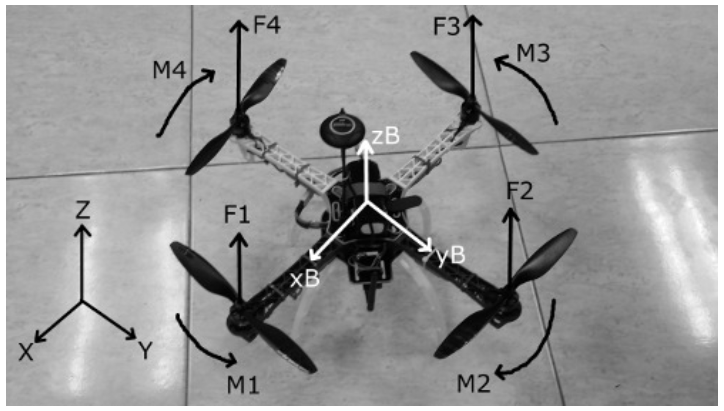
3.1. Quadrotor’s Dynamic Model
3.2. Trajectory Tracking of a Quadrotor
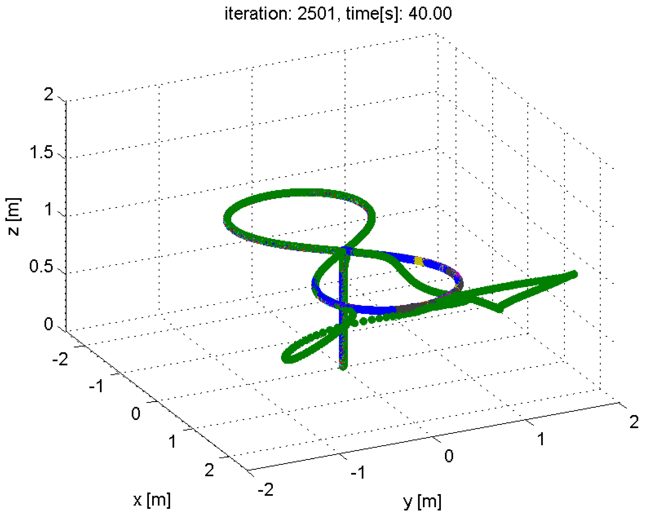
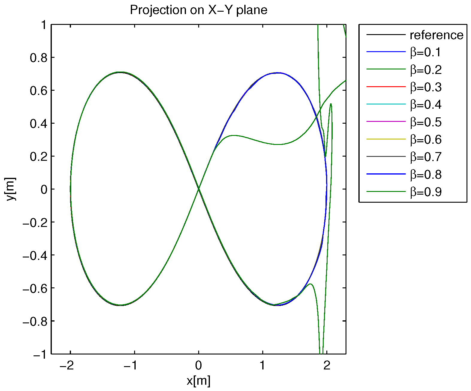
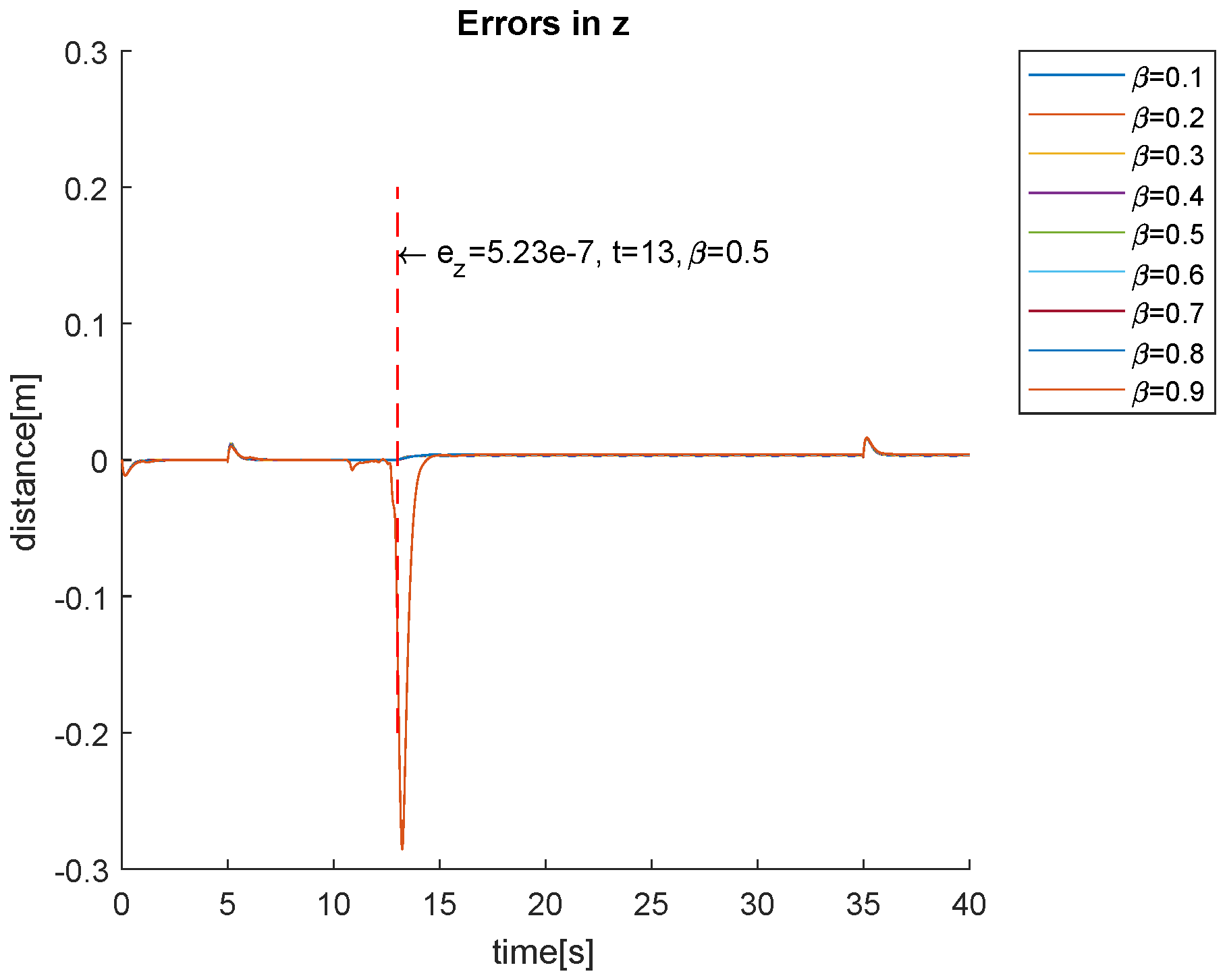
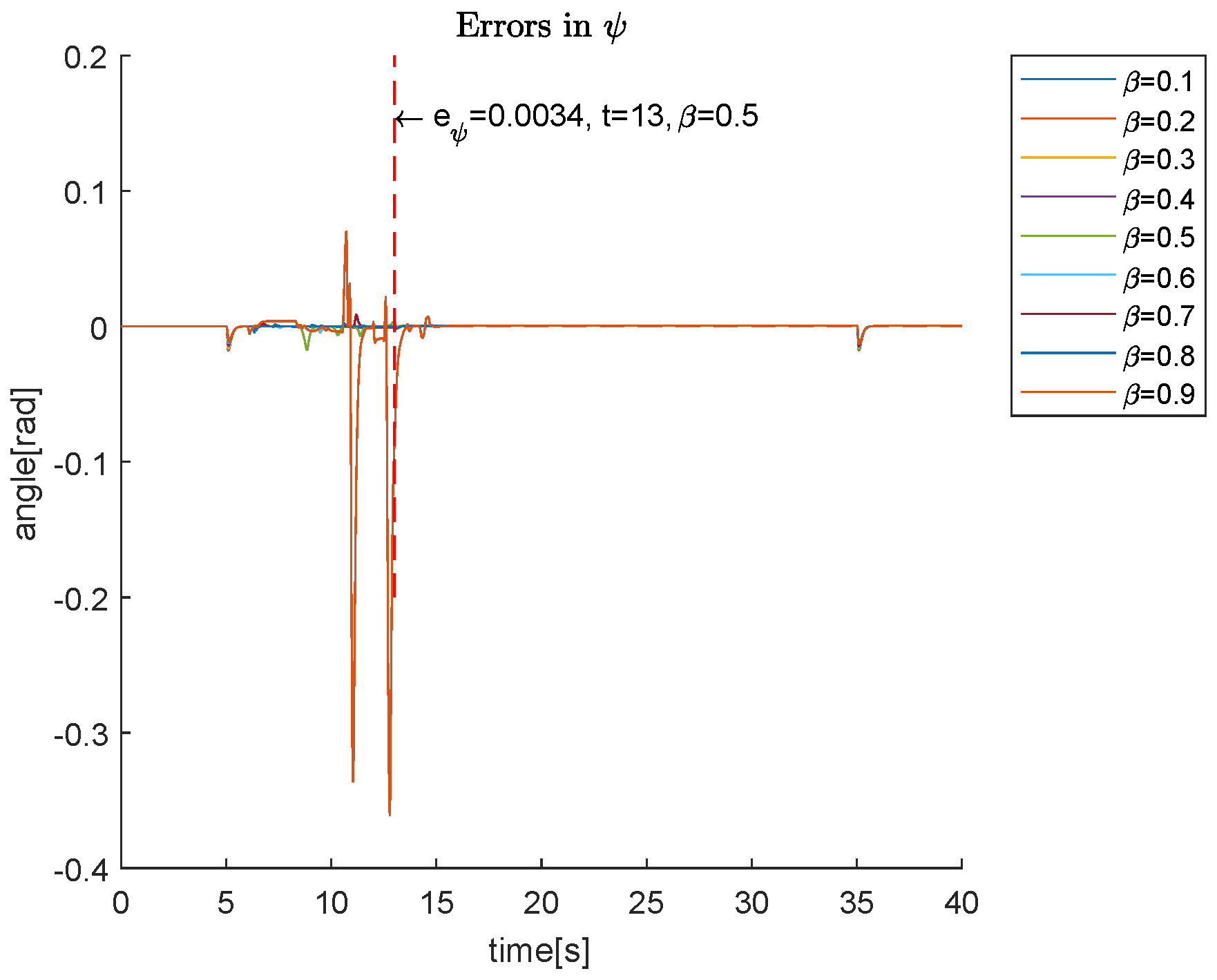
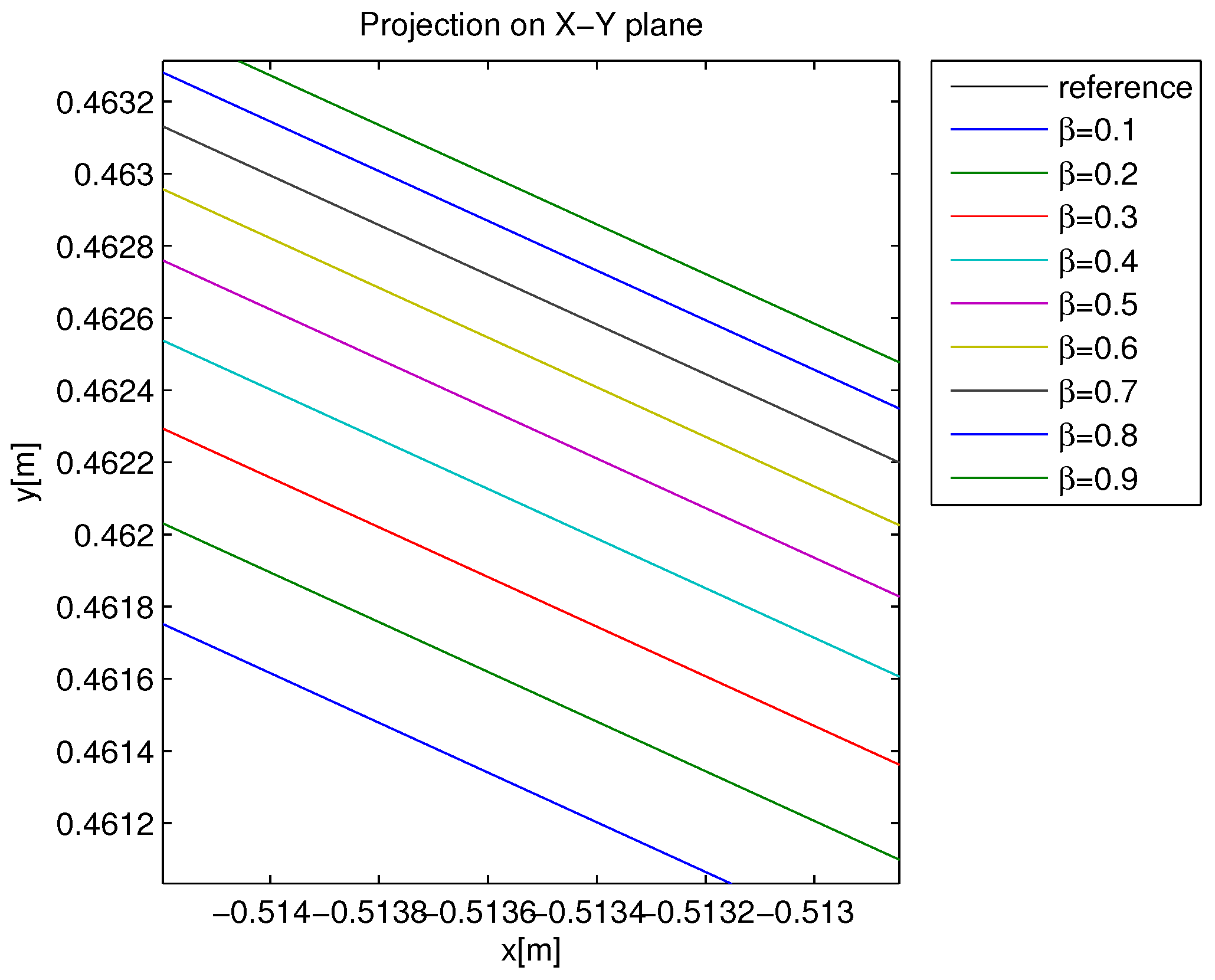
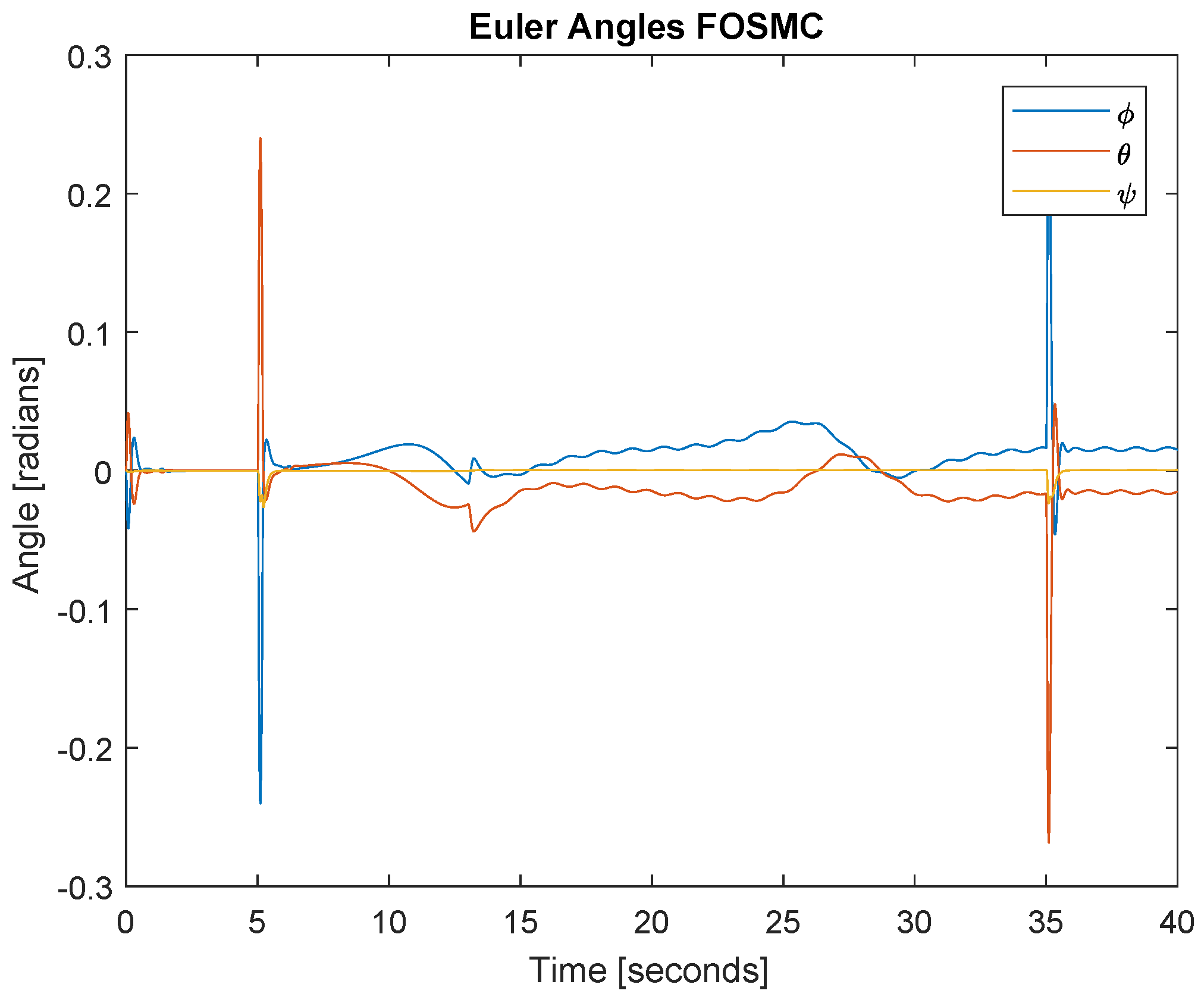
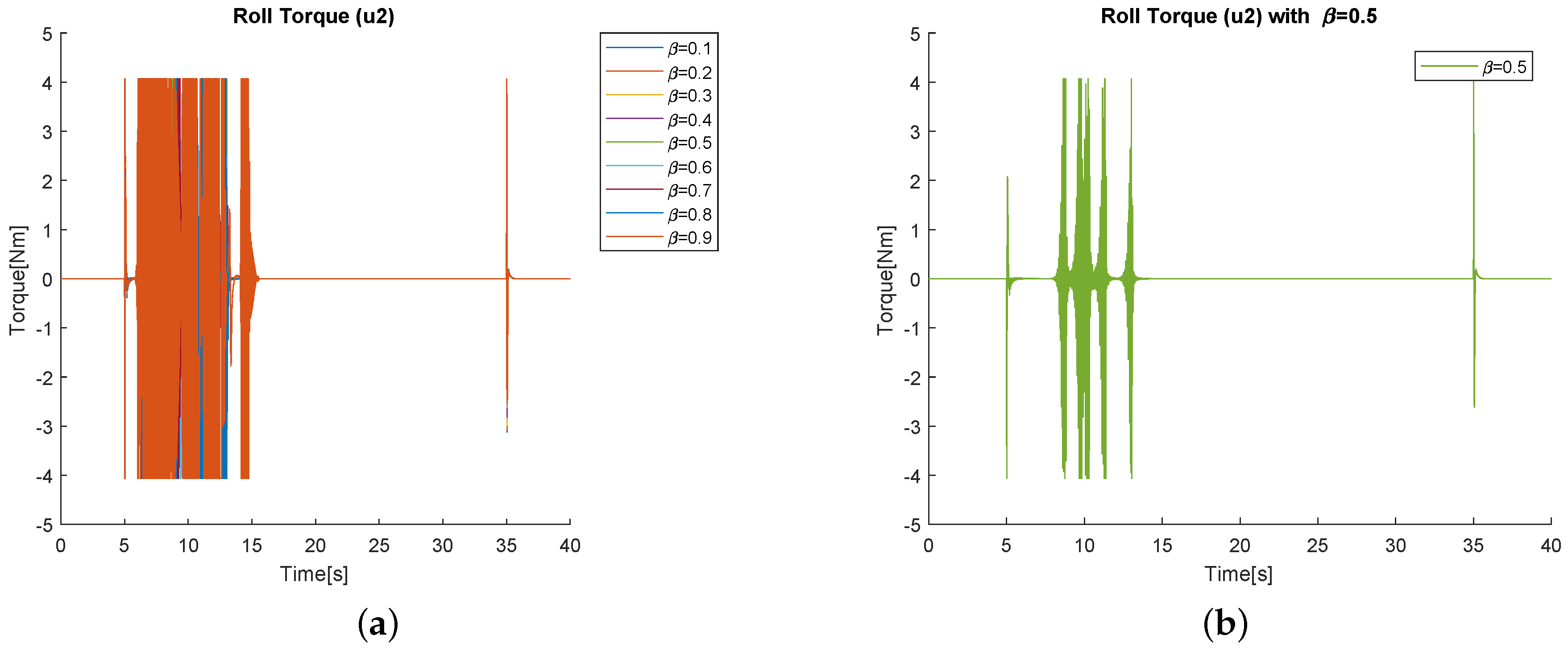
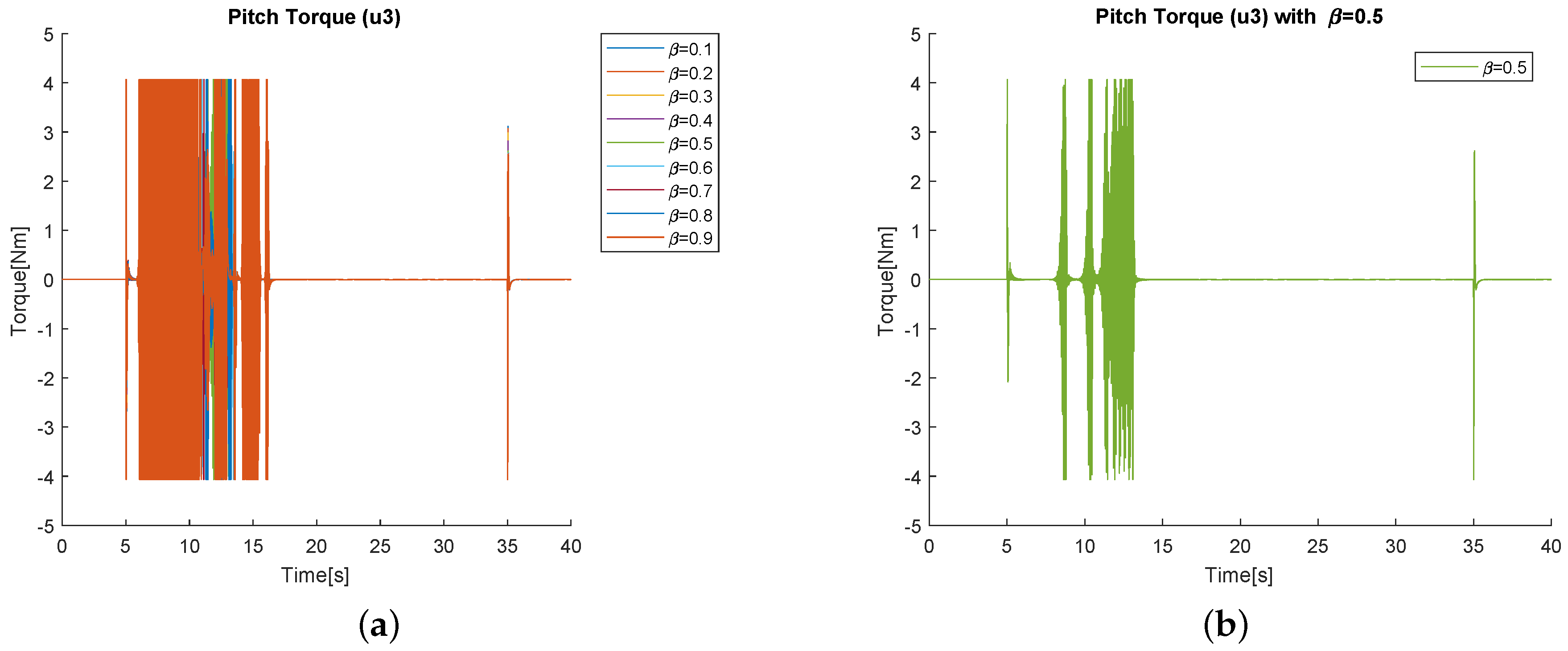
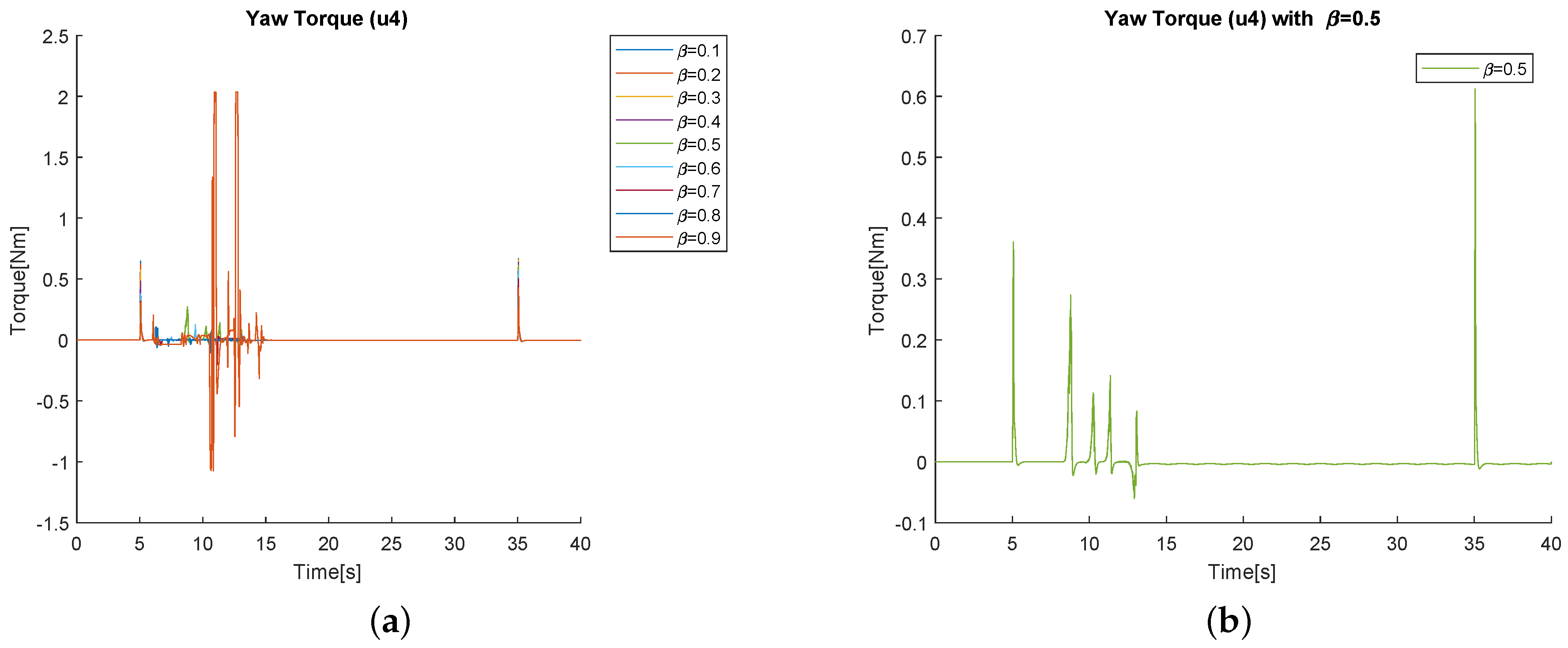
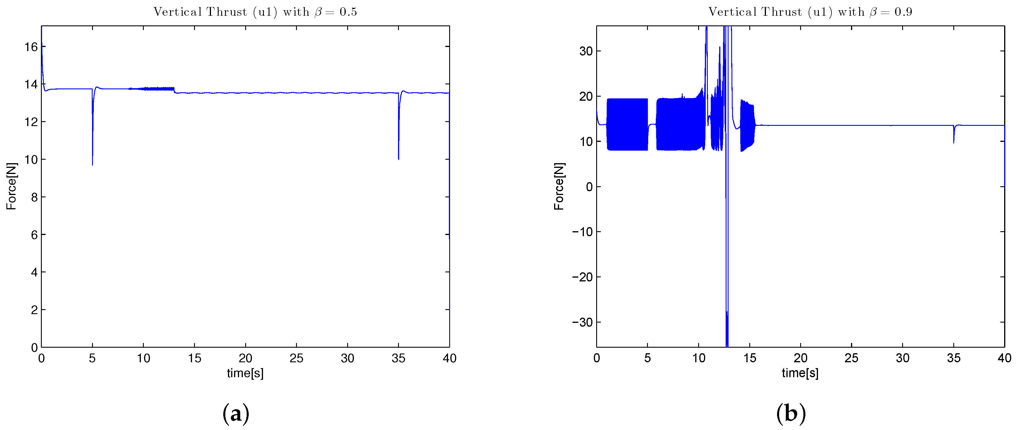
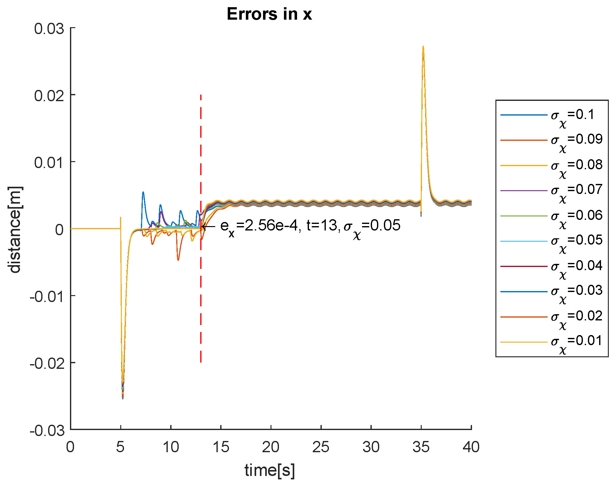
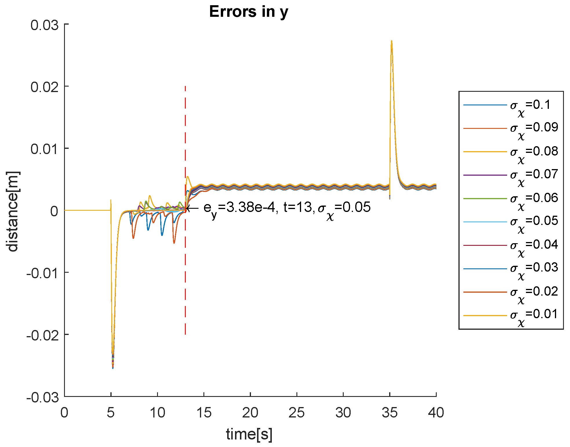
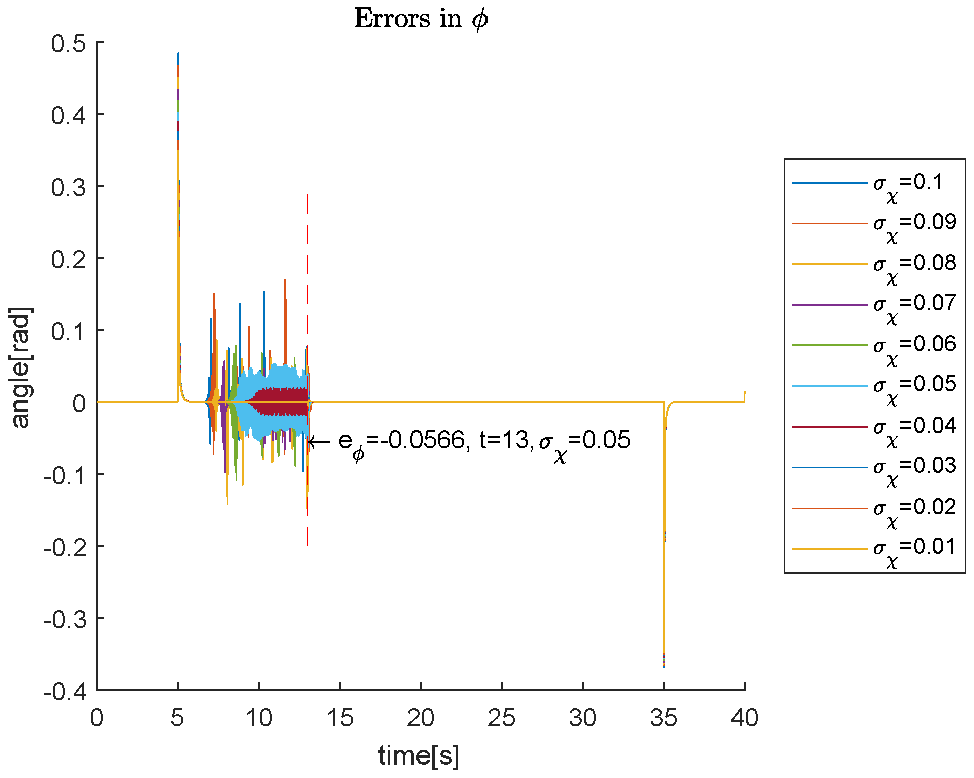
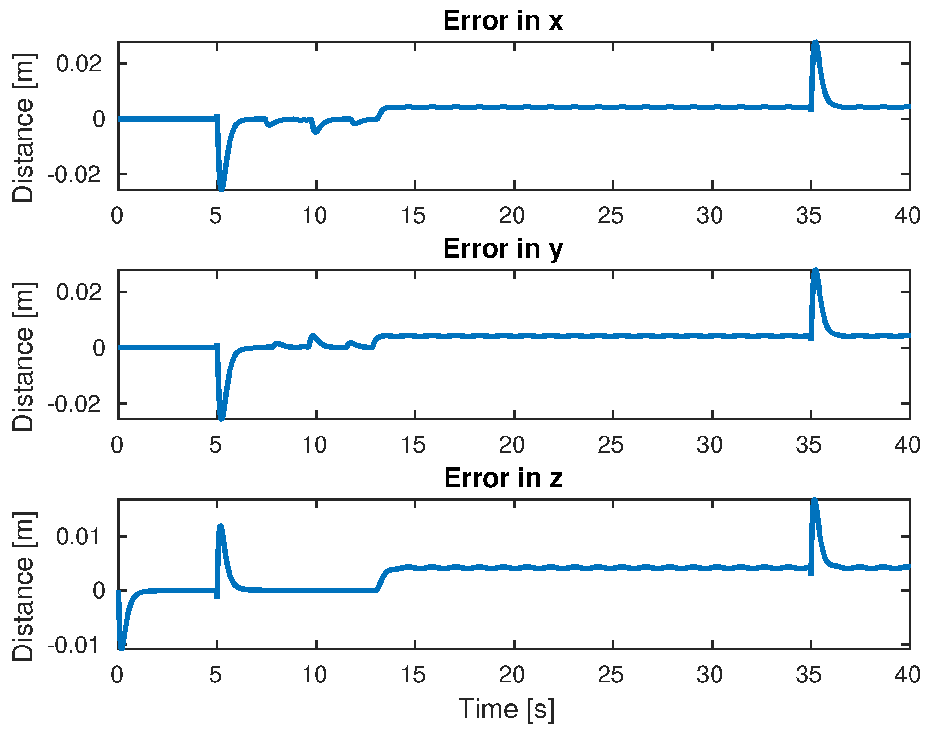
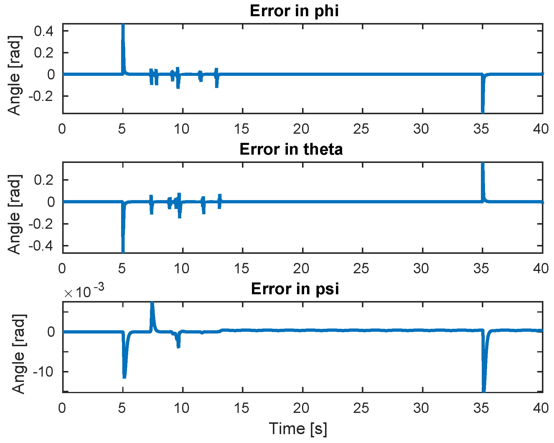
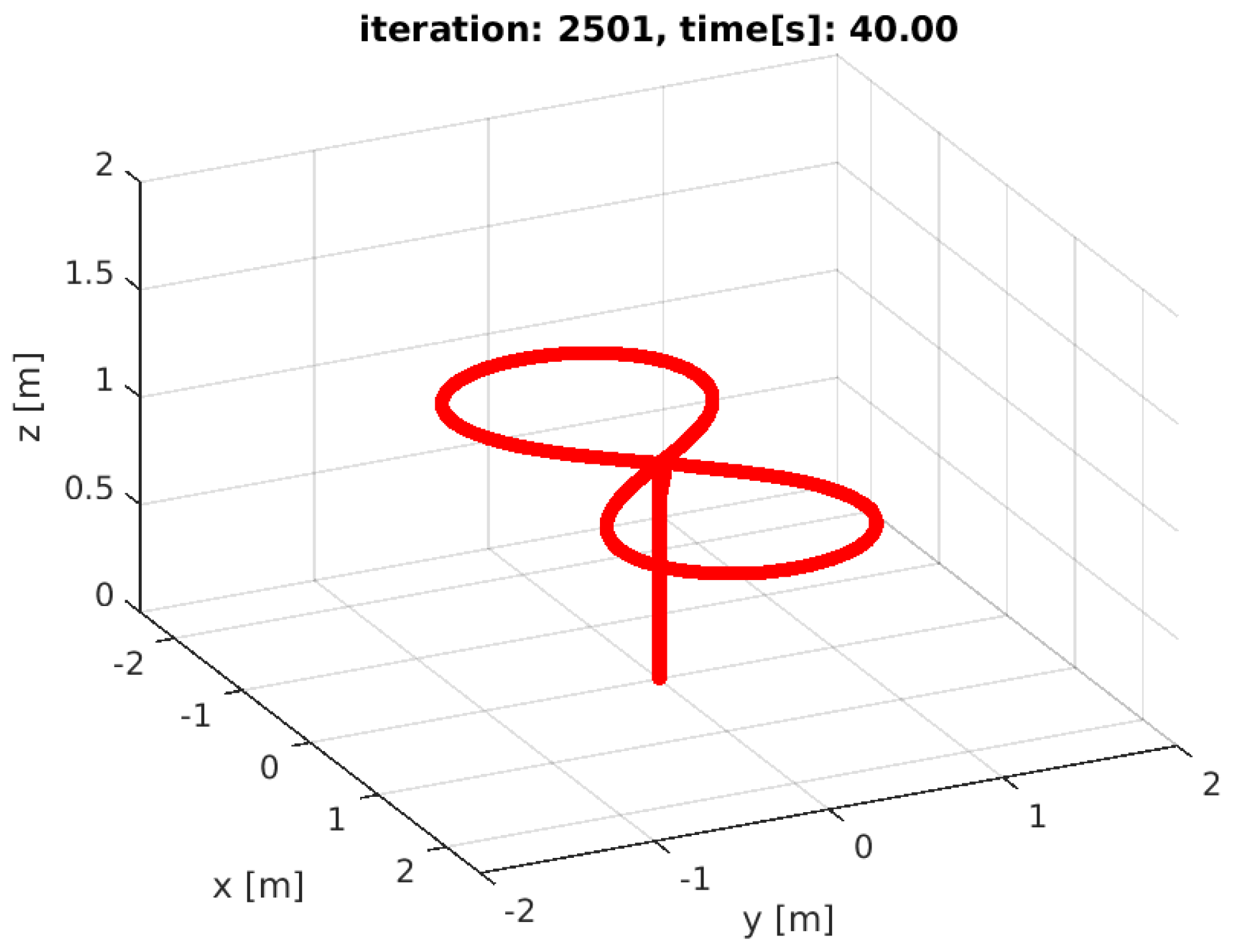
4. Simulation Results
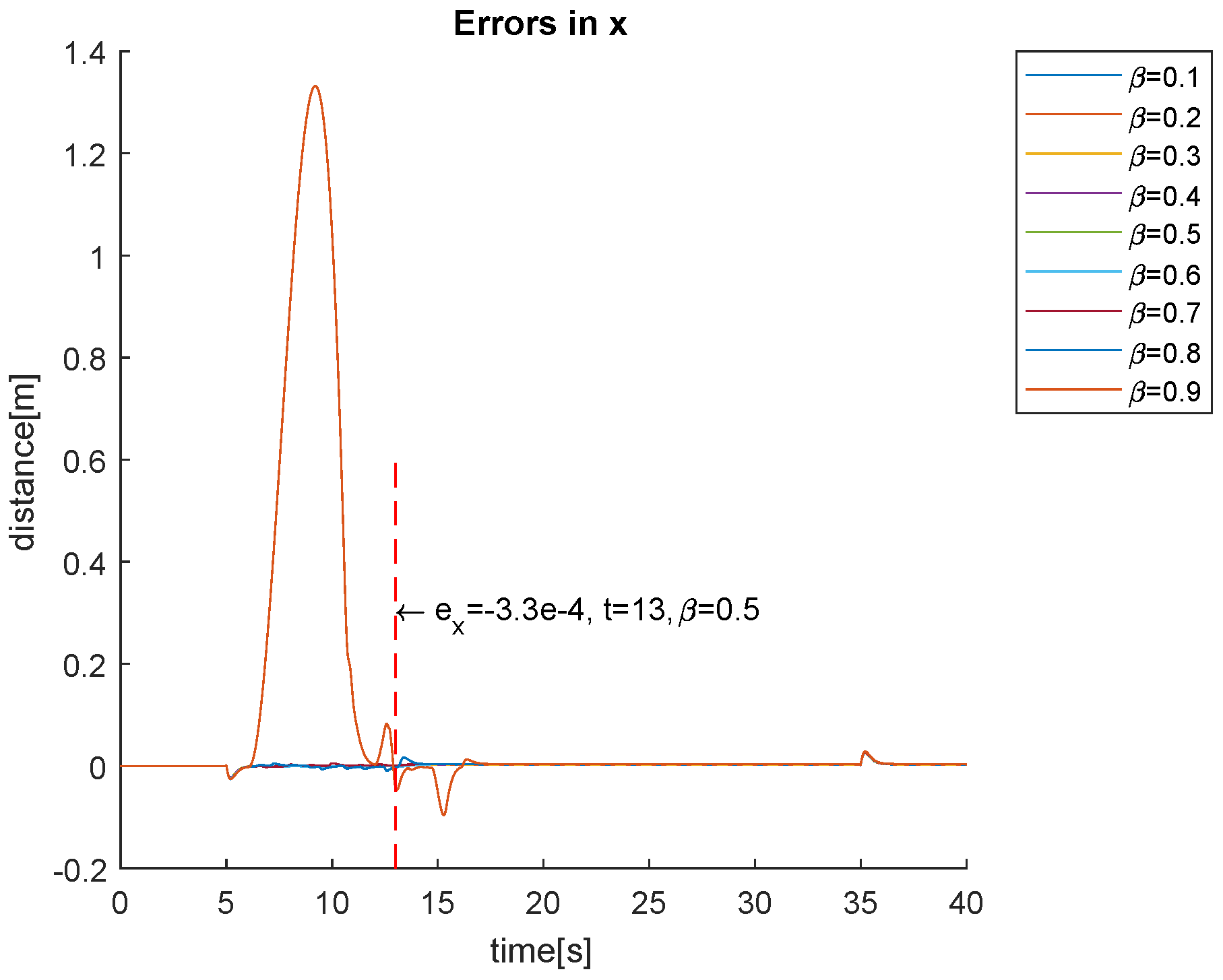
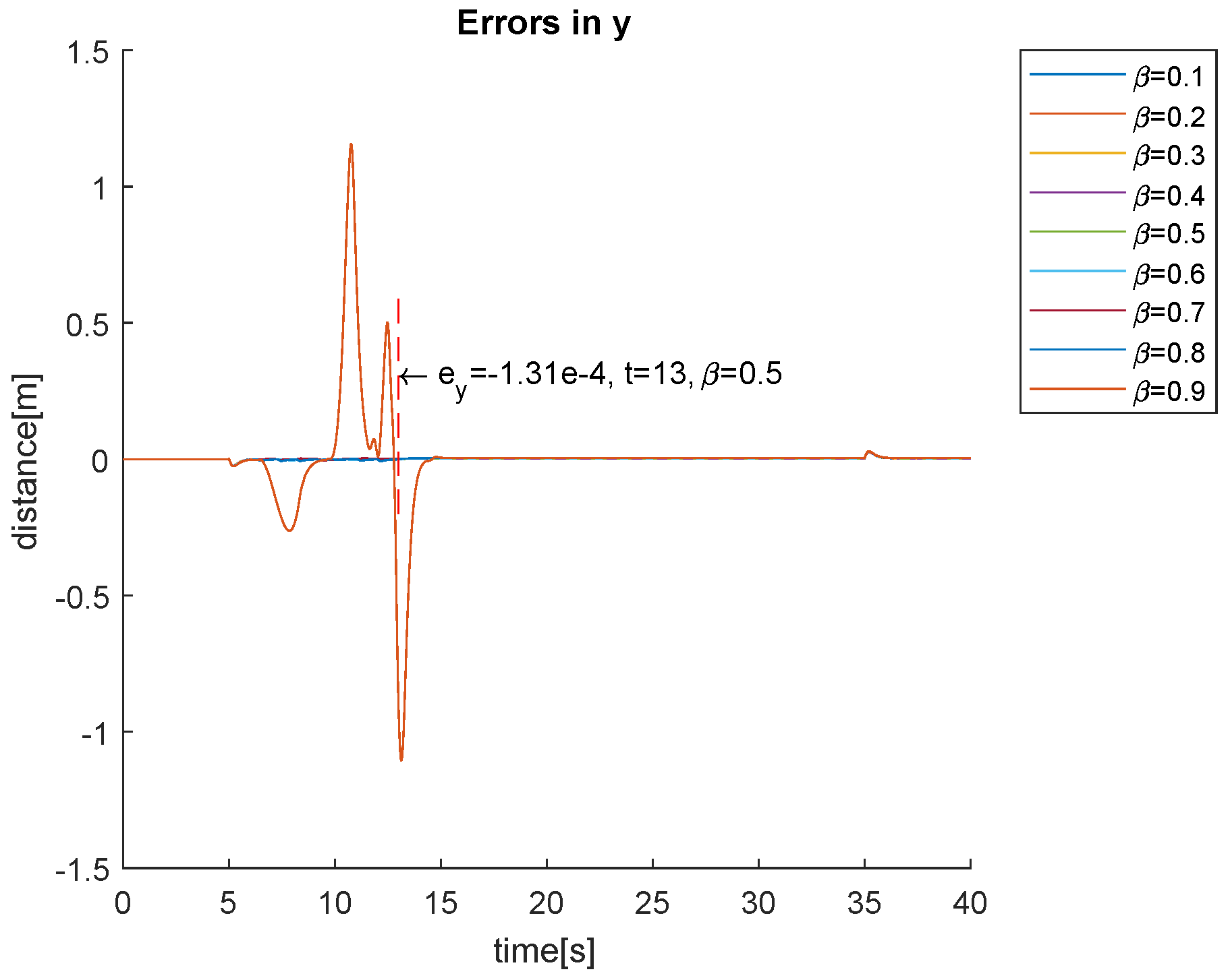
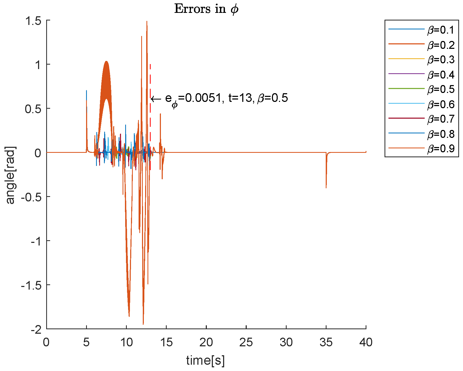
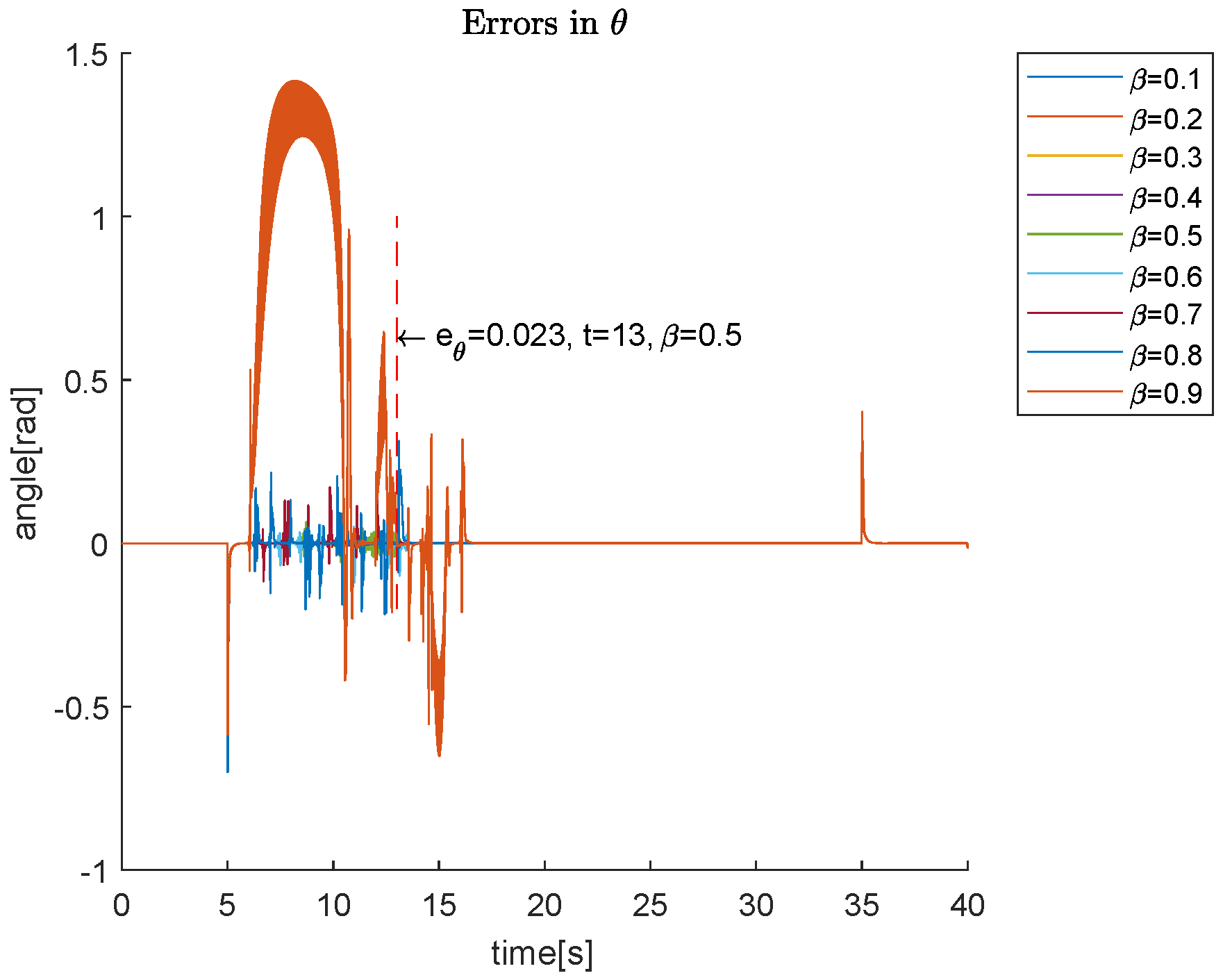
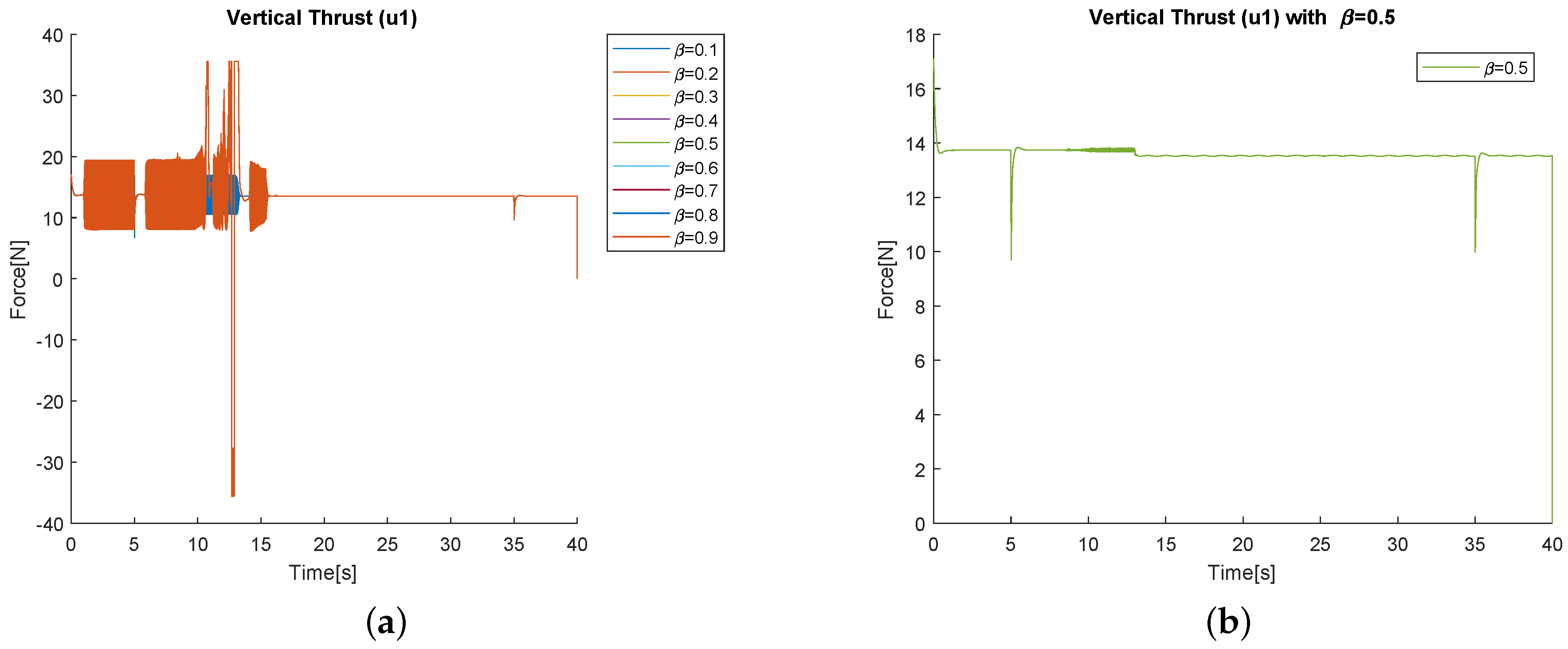
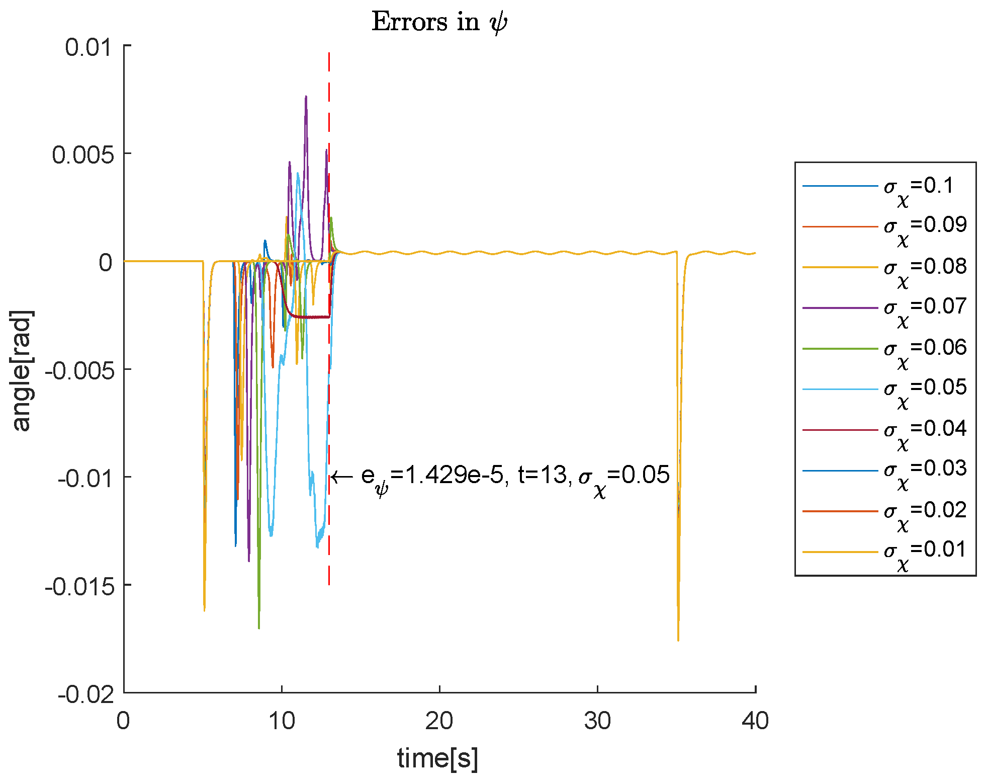
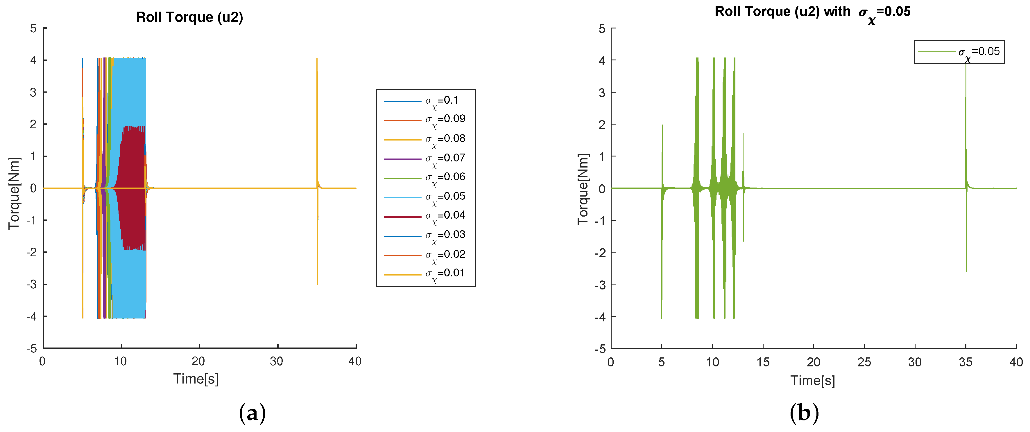
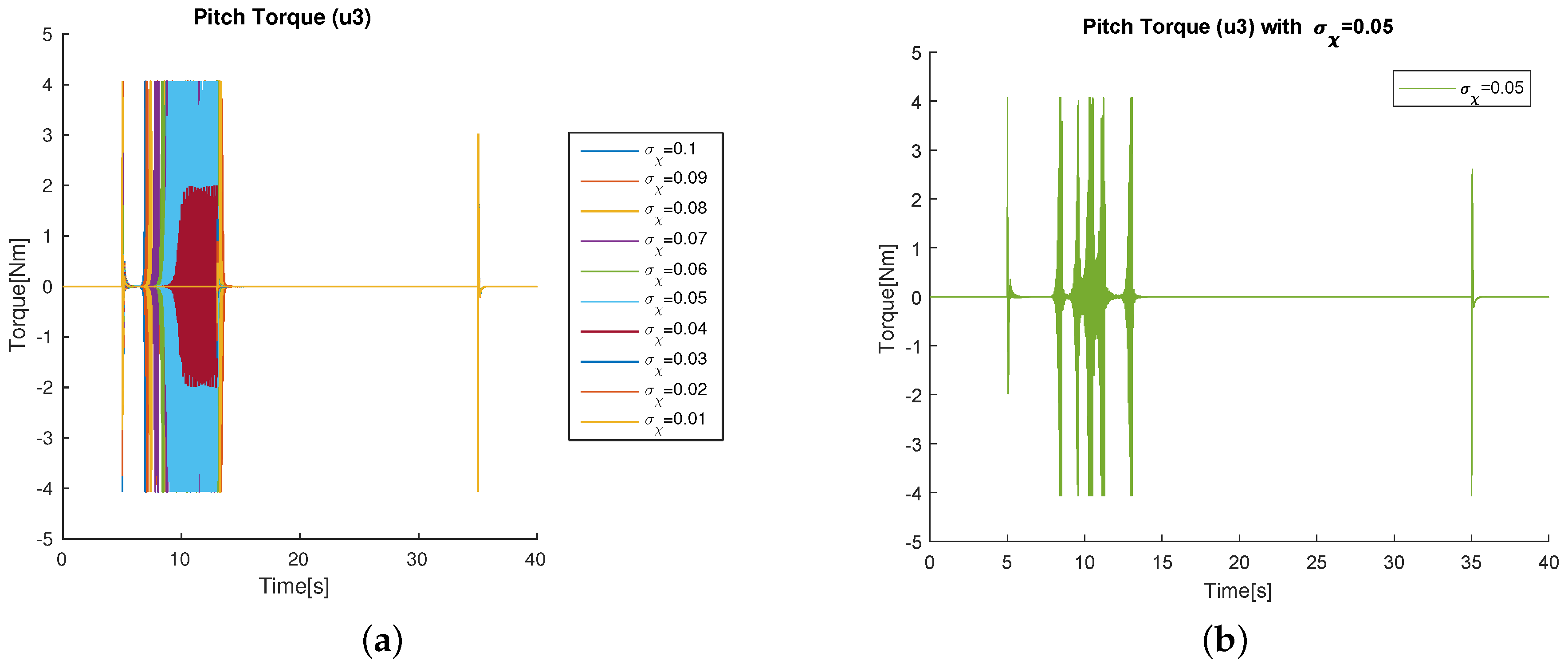
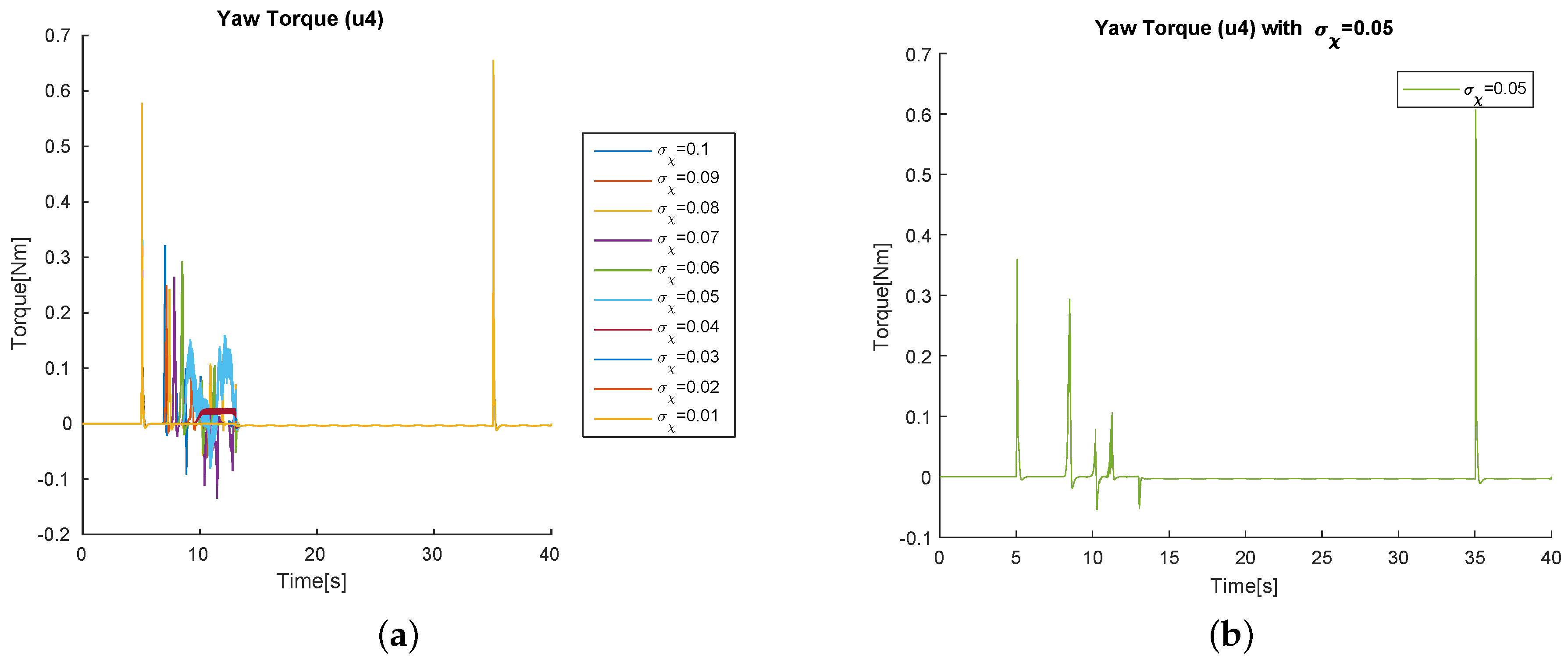
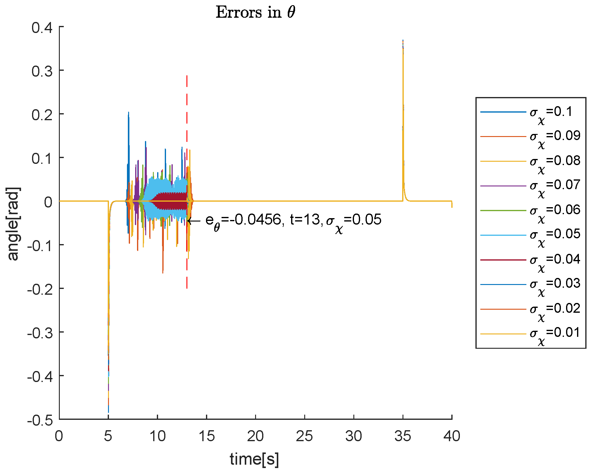
4.1. Simulations Varying the Parameters
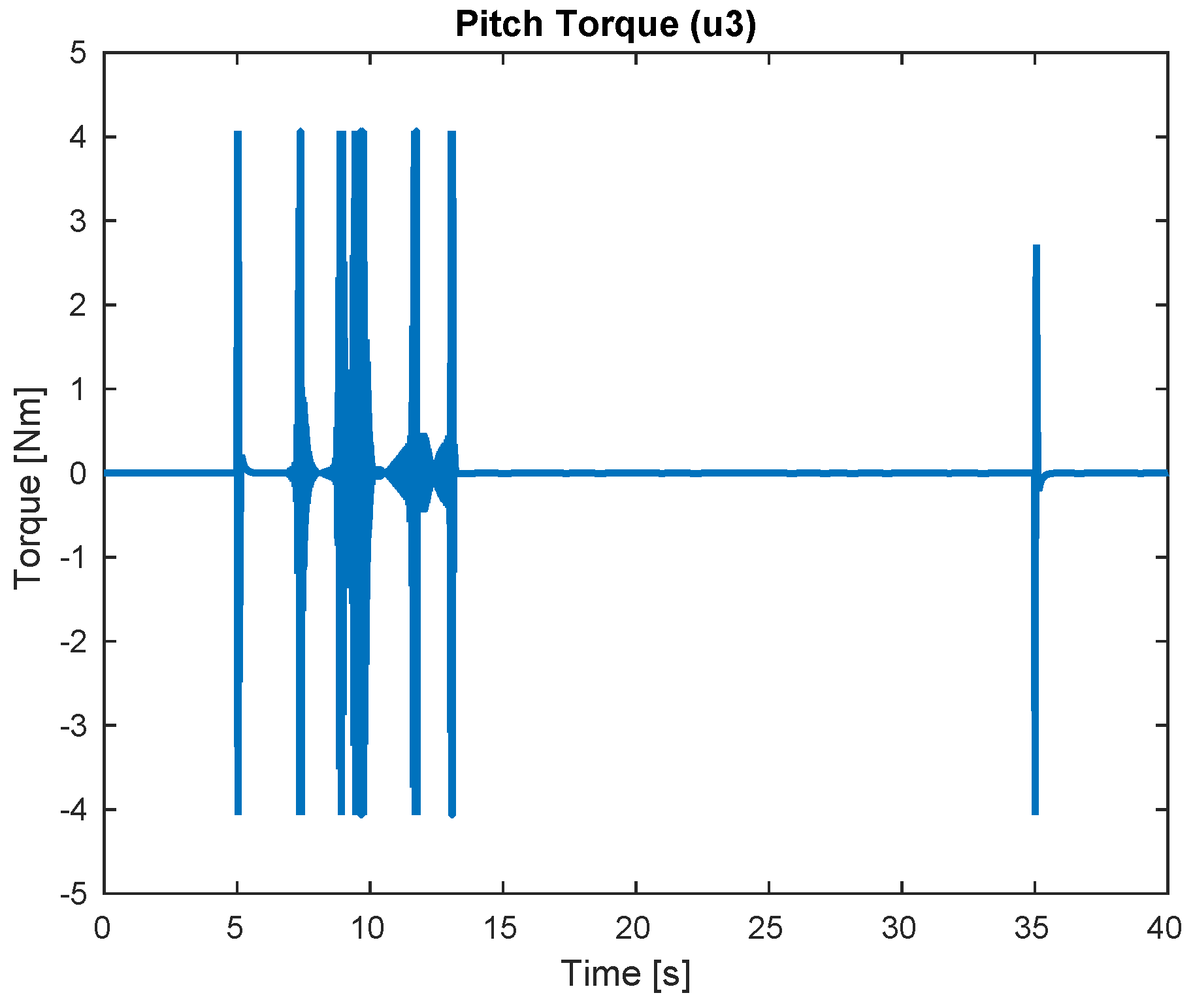
4.2. Comparison with the IOSMC
5. Conclusions
Author Contributions
Funding
Acknowledgments
Conflicts of Interest
References
- Oustaloup, A. From Fractality to Non Integer Derivation: A Fundamental Idea for a New Process Control Strategy. Anal. Optim. Syst. 2006, 53–64. [Google Scholar] [CrossRef]
- Podlubny, I.; Dorcak, K.; Kostial, I. On fractional derivatives, fractional-order dynamic systems and PIλDμ controllers. In Proceedings of the Conference on Decision and Control, San Diego, CA, USA, 10–12 December 1997; pp. 4985–4990. [Google Scholar]
- Podlubny, I. Fractional-order systems and PIλDμ controllers. IEEE Trans. Autom. Control 1999. [Google Scholar] [CrossRef]
- Lurie, B.J. Three Parameter Tunable Tilt-Integral Derivative (TID) Controller. US Patent US5371 670, 6 December 1994. [Google Scholar]
- Monje, C.A.; Calderon, A.J.; Vinagre, B.M. The fractional order lead compensator. In Proceedings of the IEEE International Conference on Computational Cybernetics, Vienna, Austria, 30 August–1 September 2004; pp. 347–352. [Google Scholar]
- Tavazoei, M.S.; Tavakoli-Kakhki, M. Compensation by fractional-order phase-lead/lag compensators. IET Control Theory Appl. 2014. [Google Scholar] [CrossRef]
- Federico, S.F.; Torres, F.M. Fractional conservation laws in optimal control theory. Nonlinear Dyn. 2008. [Google Scholar] [CrossRef]
- Agrawal, C.; Chen, Y.Q. An approximate method for numerically solving fractional-order optimal control problems of general. Comput. Math. Appl. 2010. [Google Scholar] [CrossRef]
- Ladcai, S. Charef On fractional adaptive control. Nonlinear Dyn. 2006. [Google Scholar] [CrossRef]
- Aguila-Camacho, N.; Duarte-Mermoud, M.A. Fractional adaptive control for automatic voltage regulator. ISA Trans. 2013, 52, 807–815. [Google Scholar] [CrossRef] [PubMed]
- Utkin, V.I. Sliding Modes in Optimization and Control Problems; Springer: New York, NY, USA, 1992; ISBN 978-3-642-84379-2. [Google Scholar]
- Fridman, L. An averaging approach to chattering. IEEE Trans. Autom. Control 2001, 46, 1260–1265. [Google Scholar] [CrossRef]
- Slotine, J.J.E.; Li, W. Applied Nonlinear Control; Prentice Hall Inc.: London, UK, 1991; ISBN-13 978-0130408907. [Google Scholar]
- Dadras, S.; Momeni, H.R. Fractional terminal sliding mode control design for a class of dynamical systems with uncertainty. Commun. Nonlinear Sci. Numer. Simul. 2012. [Google Scholar] [CrossRef]
- Mujumdar, A.; Kurode, S.; Tamhane, B. Fractional-order sliding mode control for single link flexible manipulator. IEEE Int. Conf. Control Appl. 2013. [Google Scholar] [CrossRef]
- Tang, Y.G.; Zhang, X.; Zhang, D.; Zhao, G.; Guan, X. Fractional-order sliding mode controller design for antilock braking systems. Neurocomputing 2013, 111, 122–130. [Google Scholar] [CrossRef]
- Tang, Y.G.; Wang, Y.; Han, M.Y.; Lian, Q. Adaptive fuzzy fractional-order sliding mode controller design for antilock braking systems. Neurocomputing 2016, 138. [Google Scholar] [CrossRef]
- Zhang, B.T.; Pi, Y.G.; Luo, Y. Fractional-order sliding mode control based on parameter auto-tuning for velocity control of permanent magnet sychronous motor. ISA Trans. 2012. [Google Scholar] [CrossRef] [PubMed]
- Aghababa, M.P. A fractional-order controller for vibration suppression of uncertain structures. ISA Trans. 2013. [Google Scholar] [CrossRef] [PubMed]
- Shao, S.Y.; Chen, M.; Yan, X.H. Adaptive sliding mode synchronization for a class of fractional-order chaotic systems with disturbance. Nonlinear Dyn. 2016. [Google Scholar] [CrossRef]
- Shao, S.Y.; Chen, M.; Chen, S.D.; Wu, Q. Adaptive neural control for an uncertain fractional-order rotational mechanical system using disturbance observer. IET Control Theory Appl. 2016, 10, 1972–9180. [Google Scholar] [CrossRef]
- Önder-Efe, M. A sufficient condition for checking the attractiveness of a sliding manifold in fractional order sliding mode control. Asian J. Control 2011, 1118–1122. [Google Scholar] [CrossRef]
- Aguila-Camacho, N.; Duarte-Mermoud, M.A.; Gallegos, J.A. Lyapunov functions for fractional order systems. Commun. Nonlinear Sci. Numer. Simul. 2014, 19, 2951–2957. [Google Scholar] [CrossRef]
- Yu, X.; Önder Efe, M. Recent Advances in Sliding Modes: From Control to Intelligent Mechatronics; Springer Internation Publishing: Basel, Switzerland, 2015; ISBN 978-3-319-18290-2. [Google Scholar]
- Önder-Efe, M. Integral sliding mode control of a quadrotor with fractional order reaching dynamics. Trans. Inst. Meas. Control 2010, 985–1003. [Google Scholar] [CrossRef]
- Önder-Efe, M. Fractional order sliding mode control with reaching law approach. Acad. J. 2010, 731–747. [Google Scholar] [CrossRef]
- García Carrillo, L.R.; Dzul López, A.E.; Lozano, R.; Pégard, C. Quad Rotorcraft Control. Vision Based Hovering and Navigation; Springer-Verlag: London, UK, 2013; ISBN 978-1-4471-4399-4. [Google Scholar]
- Reinoso, M.; Minchala, L.I.; Ortiz, J.P.; Astudillo, D.; Verdugo, D. Trajectory Tracking of a Quadrotor Using Sliding Mode Control. IEEE Latin Am. Trans. 2016, 2157–2166. [Google Scholar] [CrossRef]
- Daniel Warren, M. Trajectory Generation and Control for Quadrotors. Publicly Accessible Penn Dissertations. 2012. Available online: https://repository.upenn.edu/edissertations/547/ (accessed on 23 October 2018).
- Guadarrama-Olvera, J.R.; Corona-Sánchez, J.J.; Rodríguez-Cortés, H. Hard Real-Time Implementation of Nonlinear Controller for the Quadrotor Helicopter. J. Intell. Robot. Syst. 2013, 73, 81–97. [Google Scholar] [CrossRef]
- MacDonald, C.L.; Bhattacharya, N.; Sprouse, B.P.; Silva, G.A. Efficient computation on the Grünwald-Letnikov fractional diffusion derivative using adaptive time step memory. J. Comput. Phys. 2015, 221–236. [Google Scholar] [CrossRef]
- Andrew, N. Linear and Non-Linear Control of a Quadrotor UAV. All Theses. 2017. Available online: https://tigerprints.clemson.edu/all_theses/88/ (accessed on 23 October 2018).


| Parameter | Value | Units |
|---|---|---|
| Mass m | 1.4 | kg |
| Gravity g | 9.81 | |
| Ixx | 0.02 | kg·m |
| Iyy | 0.02 | kg·m |
| Izz | 0.04 | kg·m |
| Name | Value |
|---|---|
| 0.005 | |
| 0.055 | |
| 6.0 | |
| 6.0 | |
| 0.055 | |
| 6.0 | |
| 6.0 | |
| 0.055 | |
| 6.0 | |
| 6.0 | |
| 1.5 | |
| 25 | |
| 1.5 | |
| 25 | |
| 1.3 | |
| 9 |
| Fractional Order | Color |
|---|---|
| 0.1 | Blue |
| 0.2 | Green |
| 0.3 | Red |
| 0.4 | Cyan |
| 0.5 | Purple |
| 0.6 | Yellow |
| 0.7 | Brown |
| 0.8 | Dark Blue |
| 0.9 | Light Green |
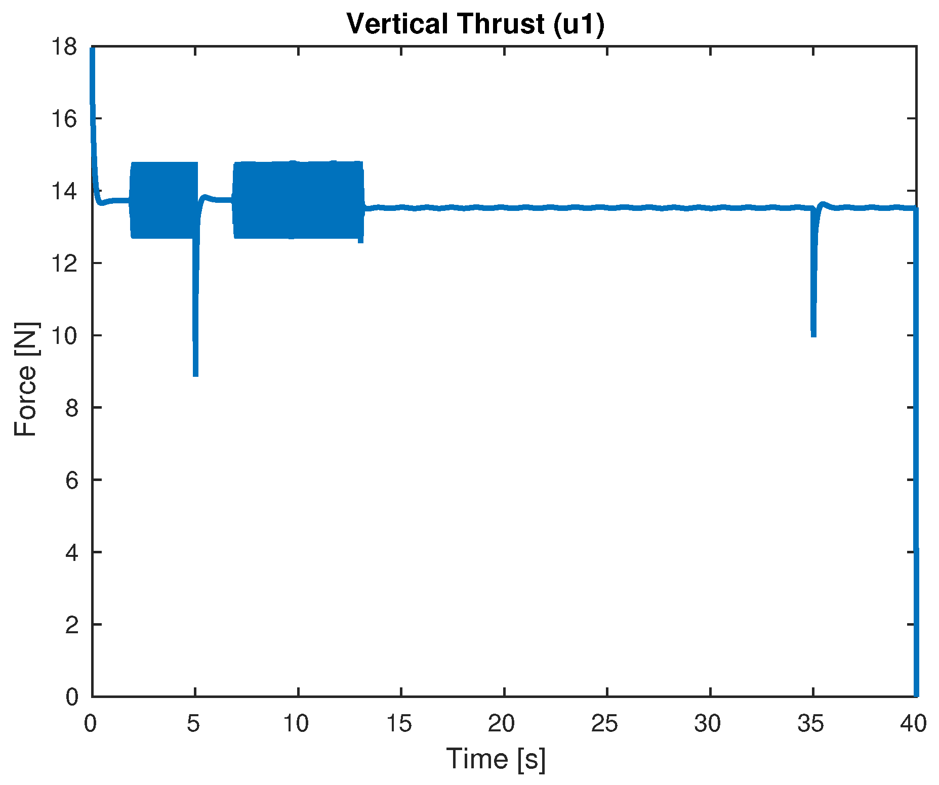
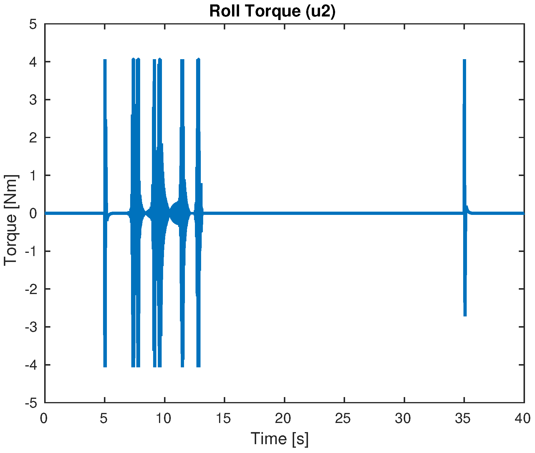
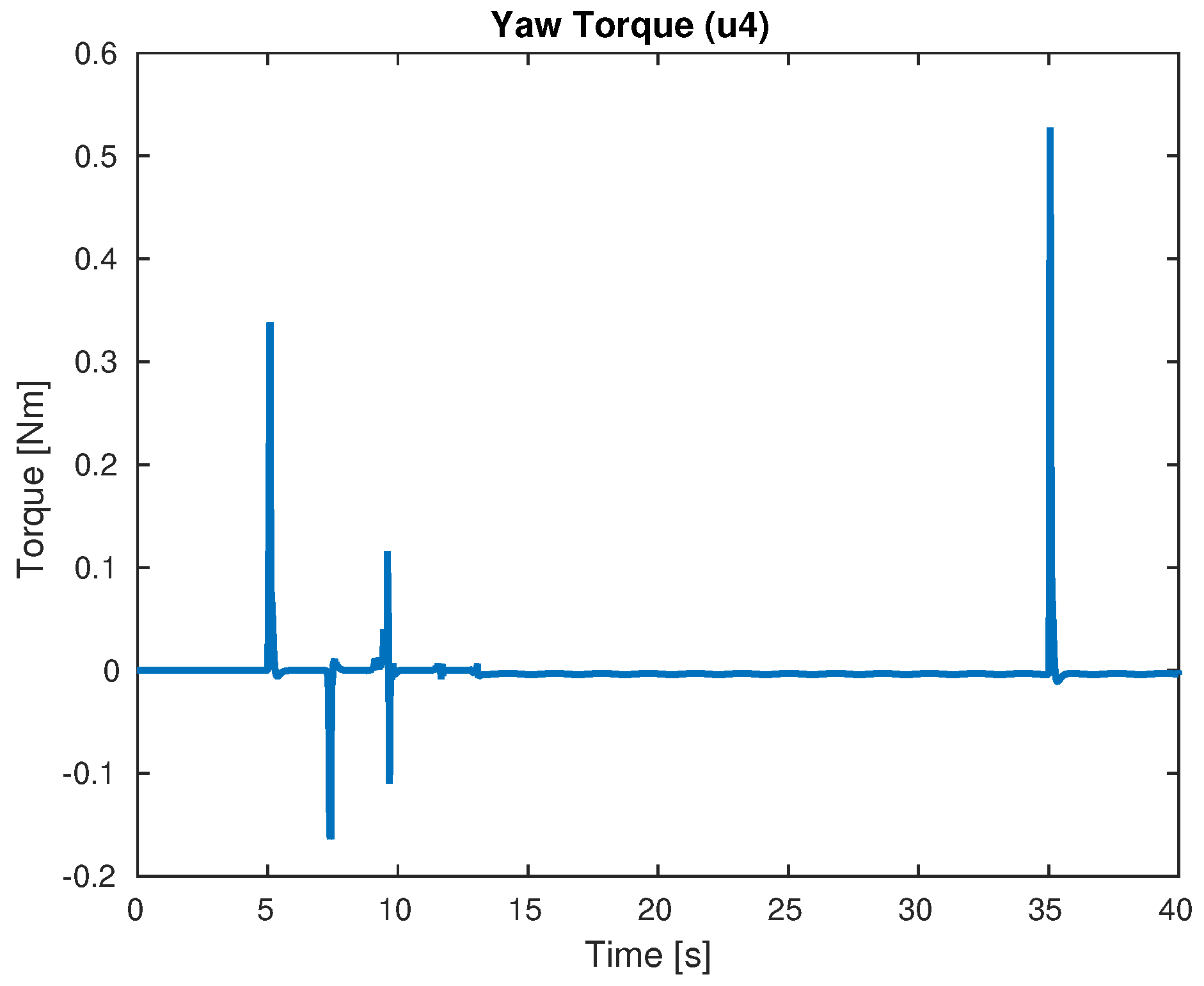
| Signal | Maximal Value | Units |
|---|---|---|
| Thrust | 35 | N |
| Roll Torque | 4 | Nm |
| Pitch Torque | 4 | Nm |
| Yaw Torque | 2 | Nm |
| Name | Value |
|---|---|
| 0.005 | |
| 0.01 | |
| 6.0 | |
| 6.0 | |
| 0.01 | |
| 6.0 | |
| 6.0 | |
| 0.01 | |
| 6.0 | |
| 6.0 | |
| 1.5 | |
| 25 | |
| 1.5 | |
| 25 | |
| 1.3 | |
| 9 |
© 2018 by the authors. Licensee MDPI, Basel, Switzerland. This article is an open access article distributed under the terms and conditions of the Creative Commons Attribution (CC BY) license (http://creativecommons.org/licenses/by/4.0/).
Share and Cite
Govea-Vargas, A.; Castro-Linares, R.; Duarte-Mermoud, M.A.; Aguila-Camacho, N.; Ceballos-Benavides, G.E. Fractional Order Sliding Mode Control of a Class of Second Order Perturbed Nonlinear Systems: Application to the Trajectory Tracking of a Quadrotor. Algorithms 2018, 11, 168. https://doi.org/10.3390/a11110168
Govea-Vargas A, Castro-Linares R, Duarte-Mermoud MA, Aguila-Camacho N, Ceballos-Benavides GE. Fractional Order Sliding Mode Control of a Class of Second Order Perturbed Nonlinear Systems: Application to the Trajectory Tracking of a Quadrotor. Algorithms. 2018; 11(11):168. https://doi.org/10.3390/a11110168
Chicago/Turabian StyleGovea-Vargas, Arturo, Rafael Castro-Linares, Manuel A. Duarte-Mermoud, Norelys Aguila-Camacho, and Gustavo E. Ceballos-Benavides. 2018. "Fractional Order Sliding Mode Control of a Class of Second Order Perturbed Nonlinear Systems: Application to the Trajectory Tracking of a Quadrotor" Algorithms 11, no. 11: 168. https://doi.org/10.3390/a11110168
APA StyleGovea-Vargas, A., Castro-Linares, R., Duarte-Mermoud, M. A., Aguila-Camacho, N., & Ceballos-Benavides, G. E. (2018). Fractional Order Sliding Mode Control of a Class of Second Order Perturbed Nonlinear Systems: Application to the Trajectory Tracking of a Quadrotor. Algorithms, 11(11), 168. https://doi.org/10.3390/a11110168