Width, Depth, and Space: Tradeoffs between Branching and Dynamic Programming

Abstract

Treedepth is a well-established width measure which has recently seen a resurgence of interest. Since graphs of bounded treedepth are more restricted than graphs of bounded tree- or pathwidth, we are interested in the algorithmic utility of this additional structure. On the negative side, we show with a novel approach that the space consumption of any (single-pass) dynamic programming algorithm on treedepth decompositions of depth d cannot be bounded by ${(2-ϵ)}^d·{log}^{O\left(1\right)}n$ for Vertex Cover, ${(3-ϵ)}^d·{log}^{O\left(1\right)}n$ for 3-Coloring and ${(3-ϵ)}^d·{log}^{O\left(1\right)}n$ for Dominating Set for any $ϵ>0$. This formalizes the common intuition that dynamic programming algorithms on graph decompositions necessarily consume a lot of space and complements known results of the time-complexity of problems restricted to low-treewidth classes. We then show that treedepth lends itself to the design of branching algorithms. Specifically, we design two novel algorithms for Dominating Set on graphs of treedepth d: A pure branching algorithm that runs in time $d^{O(d^2)}·n$ and uses space $O(d^{3}logd+dlogn)$ and a hybrid of branching and dynamic programming that achieves a running time of $O(3^{d}logd·n)$ while using $O(2^{d}dlogd+dlogn)$ space.

1. Introduction

The notion of treedepth has been introduced several times in the literature under several different names. It was arguably first formalized under the name of elimination (tree) height in the context of Cholesky factorization [1,2,3,4,5,6]. The notion has also been studied under the names of 1-partition tree [7], separation game [8], vertex ranking/ordered colorings [9,10]. Recently, Ossona de Mendez and Nešetřil brought the same concept to the limelight in the guise of treedepth in their book Sparsity [11]. Here we use a definition of treedepth that we consider easiest to exploit algorithmically: The treedepth $\mathbf{td}\left(G\right)$ of a graph G is the minimal height of a rooted forest F such that G is a subgraph of the closure of F. The closure of a forest is the graph resulting from adding edges between every node and its ancestors, i.e., making every path from root to leaf into a clique. A treedepth decomposition is a forest witnessing this fact.

Algorithmically, treedepth is interesting since it is structurally more restrictive than pathwidth. Treedepth bounds the pathwidth and treewidth of a graph, i.e., $\mathbf{tw}\left(G\right)\le \mathbf{pw}\left(G\right)\le \mathbf{td}\left(G\right)-1\le \mathbf{tw}\left(G\right)·logn$, where $\mathbf{tw}\left(G\right)$ and $\mathbf{pw}\left(G\right)$ are the treewidth and pathwidth of an n-vertex graph G respectively. Furthermore, a path decomposition can be easily computed from a treedepth decomposition. There are problems that are $W\left[1\right]$-hard or remain $\mathrm{NP}$-hard when parameterized by treewidth or pathwidth, but become fixed parameter tractable (fpt) when parameterized by treedepth [12,13,14,15]; low treedepth can also be exploited to count the number of appearances of different substructures, such as matchings and small subgraphs, much more efficiently [16,17].

Lokshtanov, Marx and Saurabh showed—assuming the Strong Exponential Time Hypothesis (SETH)—that for 3-Coloring, Vertex Cover and Dominating Set algorithms on a tree decomposition of width w with running time $O(3^w·n)$, $O(2^w·n)$ and $O(3^w{w}^2·n)$, respectively, are basically optimal [18]. Their stated intent (as reflected in the title of the paper) was to substantiate the common belief that known dynamic programming algorithms (DP algorithms) that solve these problems where optimal. This is why we feel that a restriction to a certain type of algorithm is not necessarily inferior to a complexity-based approach. Indeed, most algorithms leveraging treewidth are dynamic programming algorithms or can be equivalently expressed as such [19,20,21,22,23,24]. Even before dynamic programming on tree-decompositions became an important subject in algorithm design, similar concepts were already used implicitly [25,26]. The sentiment that the table size is the crucial factor in the complexity of dynamic programming algorithms is certainly not new (see e.g., [27]), so it seems natural to provide lower bounds to formalize this intuition. Our tool of choice will be a family of boundaried graphs that are distinct under Myhill–Nerode equivalence. The perspective of viewing graph decompositions as an “algebraic” expression of boundaried graphs that allow such equivalences is well-established [21,23].

It can be noted that there have been previous formalizations of common algorithmic paradigms in an attempt to investigate what different kinds of algorithms can and cannot achieve, including dynamic programming [28,29,30,31]. This allowed to prove lower bounds for the number of operations required for certain specific problems when a certain algorithmic paradigm was applied. Other research shows that for certain problems such as Steiner Tree and Set Cover an improvement over the “naive” dynamic programming algorithm implies improving exhaustive k-SAT, which would have implications related to SETH [32,33].

To formalize the notion of a dynamic programming algorithm on tree, path and treedepth decompositions, we consider algorithms that take as input a tree-, path- or treedepth decomposition of width/depth s and size n and satisfy the following constraints:

• They pass a single time over the decomposition in a bottom-up fashion;
• they use $O(f\left(s\right)·{log}^{O\left(1\right)}n)$ space; and
• they do not modify the decomposition, including re-arranging it.

While these three constraints might look stringent, they include pretty much all dynamic programming algorithm for hard optimization problems on tree or path decompositions. For that reason, we will refer to this type of algorithms simply as DP algorithms in the following.

To show the aforementioned space lower bounds, we introduce a simple machine model that models DP algorithms on treedepth decompositions and construct superexponentially large Myhill–Nerode families that imply lower bounds for Dominating Set, Vertex Cover/Independent Set and 3-Colorability in this algorithmic model. These lower bounds hold as well for tree and path decompositions and align nicely with the space complexity of known DP algorithms: for every $ϵ>0$, no DP algorithm on such decomposition of width/depth d can use space bounded by ${(3-ϵ)}^d·{log}^{O\left(1\right)}n$ for 3-coloring or Dominating Set nor ${(2-ϵ)}^d·{log}^{O\left(1\right)}n$ for Vertex Cover/Independent Set. While probably not surprising, we consider a formal proof for what previously were just widely held assumptions valuable. The provided framework should easily extend to other problems.

Consequently, any algorithmic benefit of treedepth over pathwidth and treewidth must be obtained by non-DP means. We demonstrate that treedepth allows the design of branching algorithms whose space consumption grows only polynomially in the treedepth and logarithmic in the input size. Such space-efficient algorithms are quite easy to obtain for 3-Coloring and Vertex Cover/Independent Set with running time $O(3^d·n)$ and $O(2^d·n)$, respectively, and space complexity $O(d+logn)$ and $O(d·logn)$. Our main contribution on the positive side here are two linear-fpt algorithms for Dominating Set which use more involved branching rules on treedepth decompositions. The first one runs in time $d^{O(d^2)}·n$ and uses space $O(d^{3}logd+d·logn)$. Compared to simple dynamic programming, the space consumption is improved considerably, albeit at the cost of a much higher running time. For this reason, we design a second algorithm that uses a hybrid approach of branching and dynamic programming, resulting in a competitive running time of $O(3^{d}logd·n)$ and space consumption $O(2^{d}dlogd+dlogn)$. Both algorithms are amenable to heuristic improvements.

While applying branching to treedepth seems natural, it is unclear whether it could be applied to treewidth or pathwidth. Recent work by Drucker, Nederlof and Santhanam suggests that, relative to a collapse of the polynomial hierarchy, Independent Set restricted to low-pathwidth graphs cannot be solved by a branching algorithm in fpt time [34].

The idea of using treedepth to improve space consumption is not novel. Fürer and Yu demonstrated that it is possible to count matchings using polynomial space in the size of the input [17] and a parameter closely related to the treedepth of the input. Their algorithm achieves a small memory footprint by using the algebraization framework developed by Loksthanov and Nederlof [35]. This technique was also used by Pilipczuk and Wrochna to develop an algorithm for Dominating Set which runs in time $3^d·\mathrm{poly}(n)$ (non-linear) and uses space $O(d·logn)$ [36]. Based on this last algorithm they showed that computations on treedepth decompositions correspond to a model of non-deterministic machines that work in polynomial time and logarithmic space, with access to an auxiliary stack of maximum height equal to the decomposition’s depth.

In our opinion, algorithms based on algebraization have two disadvantages: On the theoretical side, the dependency of the running and space consumption on the input size is often at least $\mathsf{\Omega }\left(n\right)$. On the practical side, using the Discrete Fourier Transform makes it hard to apply common algorithm engineering techniques, like branch and bound, which are available for branching algorithms.

2. Preliminaries

We write $N_G\left[x\right]$ to denote the closed neighbourhood of x in G and extends this notation to vertex sets via $N_G\left[S\right]:={\bigcup }_{x\in S}{N}_G\left[x\right]$. Otherwise we use standard graph-theoretic notation (see [37] for any undefined terminology). All our graphs are finite and simple and logarithms use base two. For sets $A,B,C$ we write $A\uplus B=C$ to express that $A,B$ partition C.

Definition 1 (Treedepth).

A treedepth decomposition of a graph G is a forest F with vertex set $V\left(G\right)$, such that if $uv\in E\left(G\right)$ then either u is an ancestor of v in F or vice versa. The treedepth $\mathbf{td}\left(G\right)$ of a graph G is the minimum height of any treedepth decomposition of G.

We assume that the input graphs are connected, which allows us to presume that the treedepth decomposition is always a tree. Furthermore, let x be a node in some treedepth decomposition T. We denote by $T_x$ the complete subtree rooted at x and by $P_x$ the set of ancestors of x in T (not including x). A subtree of x refers to a subtree rooted at some child of x. The treedepth of a graph G bounds its treewidth $\mathbf{tw}\left(G\right)$ and pathwidth $\mathbf{pw}\left(G\right)$, i.e., $\mathbf{tw}\left(G\right)\le \mathbf{pw}\left(G\right)\le \mathbf{td}\left(G\right)-1$ [11]. For a definition of treewidth and pathwidth see e.g., Bodlaender [19].

An s-boundaried graph ${}^{\circ }G$ is a graph G with a set $bd\left({}^{\circ }G\right)\subseteq V\left(G\right)$ of s distinguished vertices labeled 1 through s, called the boundary of ${}^{\circ }G$. We will call vertices that are not in $bd\left({}^{\circ }G\right)$ internal. By ${}^{\circ }{\mathcal{G}}_s$ we denote the class of all s-boundaried graphs. For s-boundaried graphs ${}^{\circ }{G}_1$ and ${}^{\circ }{G}_2$, we let the gluing operation ${}^{\circ }{G}_1\oplus {}^{\circ }{G}_2$ denote the s-boundaried graph obtained by first taking the disjoint union of $G_1$ and $G_2$ and then unifying the boundary vertices that share the same label. In the literature the result of gluing is often an unboundaried graph. Our definition of gluing will be more convenient in the following.

3. Myhill–Nerode Families

In this section, we introduce the basic machinery to formalize the notion of dynamic programming algorithms and how we prove lower bounds based on this notion.

First of all, we need to establish what we mean by dynamic programming (DP). DP algorithms on graph decompositions work by visiting the bags/nodes of the decomposition in a bottom-up fashion (a post-order depth-first traversal), maintaining tables to compute a solution. For decision problems, these algorithms only need to keep at most $logn$ tables in memory at any given moment (achieved in the case of treewidth by always descending first into the part of the tree decomposition with the greatest number of leaves). We propose a machine model with a read-only tape for the input that can only be traversed once, which only accepts as input decompositions presented in a valid order. This model suffices to capture known dynamic programming algorithms on path, tree and treedepth decompositions. More specifically, given a decision problem on graphs $\mathsf{\Pi }$ and some well-formed instance $(G,\xi )$ of $\mathsf{\Pi }$ (where $\xi$ encodes the non-graph part of the input), let T be a tree, path or treedepth decomposition of G of width/depth d. We fix an encoding $\widehat{T}$ of T that lists the separators provided by the decomposition in the order they are normally visited in a dynamic programming algorithm (post-order depth-first traversal of the bag/nodes of a tree/path/treedepth decomposition) and additionally encodes the edges of G contained in a separator using $O(dlogd)$ bits per bag or path. Then $(d,\widehat{T},\xi )$ is a well-formed instance of the DP decision problem ${\mathsf{\Pi }}_{\mathrm{DP}}$. Pairing DP decision problems with the following machine model provides us with a way to model DP computation over graph decompositions.

Definition 2 (Dynamic programming TM).

A DPTM M is a Turing machine with an input read-only tape, whose head moves only in one direction and a separate working tape. It accepts as inputs only well-formed instances of some DP decision problem.

Any single-pass dynamic programming algorithm that solves a DP decision problem on tree, path or treedepth decompositions of width/depth d using tables of size $f\left(d\right)$ that does not re-arrange the decomposition can be translated into a DPTM with a working tape of size $O(f(d)·logn)$. This model does not suffice to rule out algebraic techniques, since this technique, like branching, requires to visit every part of the decomposition many times [17]; or algorithms that preprocess the decomposition first to find a suitable traversal strategy.

The theorem of Myhill and Nerode is best known from formal language theory where it is used to show that a language is not regular, but is more general in its original form. For example, if we look at the language L consisting of all words $a^{n}b{a}^n$ we define the equivalence relation ≡ by defining $u\equiv v$ if $uw\in L$ iff $vw\in L$ for all $w\in {\{a,b\}}^{\ast }$. Then $a^n\not\equiv a^m$ if $n\ne m$. This means that ≡ has infinitely many equivalence classes which shows that L is not regular. To show that an automaton would need infinitely many states is only the first step and we can furthermore investigate how much space we need when reading a word of length n. In the case of L you would need $\mathsf{\Theta }\left(n\right)$ states which translates in about $logn$ bits of space. This is a typical use of the Myhill–Nerode theorem to show a space lower bound, but our goal is different: Let us assume we have a path decomposition of a graph which is read from left to right by dynamic programming. This is very similar to reading a word where the bags play the role of the characters. We want to show a lower bound in term of the size of the bags. Roughly, the size of a bag is related to the logarithm of the alphabet size because there are exponentially many graphs in the number of vertices. Our goal is to show a lower bound that is logarithmic in the length of the input times a double exponential function of the size of the bags. For this we need a family of graphs that simultaneously has several properties: (1) Each pair ${}^{\circ }{G}_1\ne {}^{\circ }{G}_2$ from the family are not equivalent in the sense of a Myhill–Nerode equivalence, i.e., there must be a graph ${}^{\circ }H$ such that ${}^{\circ }{G}_1\oplus {}^{\circ }H$ and ${}^{\circ }{G}_2\oplus {}^{\circ }H$ give different results, e.g., one is three colorable and the other is not. (2) The family has to be very big because its size is a lower bound on the index of the Myhill–Nerode relation. To show that we need at least $c^{k}g\left(n\right)$ space, the size has to be at least $2^{c^{k}g\left(n\right)}$. If, for example, we want to show that ${(3-ϵ)}^k{log}^{O\left(1\right)}\left(n\right)$ space is not sufficient, the family has to have size at least $2^{{(3-ϵ)}^k{log}^{O\left(1\right)}\left(n\right)}<2^{3^k}$. (3) All graphs in the family and H have to be small. Otherwise $2^{{(3-ϵ)}^k{log}^{O\left(1\right)}\left(n\right)}$ could be bigger than $2^{3^k}$. The size n is the size of a graph from the family glued to H.

The following notion of a Myhill–Nerode family will provide us with the machinery to prove space lower-bounds for DPTMs where the input instance is an unlabeled graph and hence for common dynamic programming algorithms on such instances. Recall that ${}^{\circ }{\mathcal{G}}_s$ denotes the class of all s-boundaried graphs.

Definition 3 (Myhill–Nerode family).

A set $\mathcal{H}\subseteq {}^{\circ }{\mathcal{G}}_s\times \mathbf{N}$ is an s-Myhill–Nerode family for a DP-decision problem ${\mathsf{\Pi }}_{\mathrm{DP}}$ if the following holds:

1. 

For every $({}^{\circ }H,q)\in \mathcal{H}$ it holds that $\left|{}^{\circ }H\right|=\left|\mathcal{H}\right|·{log}^{O\left(1\right)}\left|\mathcal{H}\right|$ and $q=2^{\left|\mathcal{H}\right|·{log}^{O\left(1\right)}\left|\mathcal{H}\right|}$.

2. 

For every subset $\mathcal{I}\subseteq \mathcal{H}$ there exists an s-boundaried graph ${}^{\circ }{G}_{\mathcal{I}}\in {}^{\circ }{\mathcal{G}}_s$ with $|{}^{\circ }{G}_{\mathcal{I}}|=|\mathcal{H}|·{log}^{O\left(1\right)}\left|\mathcal{H}\right|$ and an integer $p_{\mathcal{I}}$ such that for every $({}^{\circ }H,q)\in \mathcal{H}$ it holds that

$$({}^{\circ }{G}_{\mathcal{I}}\oplus {}^{\circ }H,p_{\mathcal{I}}+q)\notin {\mathsf{\Pi }}_{\mathrm{DP}}\iff ({}^{\circ }H,q)\in \mathcal{I}.$$

Let ${}^{\circ }\mathbf{td}({}^{\circ }G)$ be the minimal depth over all treedepth decompositions of ${}^{\circ }G\in {\mathcal{G}}_s$ where the boundary appears as a path starting at the root. We define the size of a Myhill–Nerode family $\mathcal{H}$ as $\left|\mathcal{H}\right|$, its treedepth as

$$\mathbf{td}\left(\mathcal{H}\right)=\underset{({}^{\circ }H,·)\in \mathcal{H},\mathcal{I}\subseteq \mathcal{H}}{max}{}^{\circ }\mathbf{td}({}^{\circ }{G}_{\mathcal{I}}\oplus {}^{\circ }H)$$

and its treewidth and pathwidth as the maximum tree/path decomposition of lowest width of any $({}^{\circ }H,·)\in \mathcal{H}$ where the boundary is contained in every bag.

The following lemma still holds if we replace “treedepth” by “pathwidth” or “treewidth”.

Lemma 1.

Let $ϵ>0,c>1$ and Π be a DP decision problem such that for every s there exists an s-Myhill–Nerode family $\mathcal{H}$ for Π of size $c^s/f\left(s\right)$ where $f\left(s\right)=s^{O\left(1\right)}$ and depth $\mathbf{td}\left(\mathcal{H}\right)=s+o\left(s\right)$. Then no DPTM can decide Π using space $O({(c-ϵ)}^k·{log}^{O\left(1\right)}n)$, where n is the size of the input instance and k the depth of the treedepth decomposition given as input.

Before proving Lemma 1 let us look at a simple example. The DP decision problem consists of graphs that have components of size s and there are not two components that are isomorphic. Let $\mathcal{H}$ be a set of $c^s$ different $({}^{\circ }G,1)$ where ${}^{\circ }G$ is a graph of size s with an empty boundary. Then $\mathcal{H}$ is an s-Myhill–Nerode family: The size constraints are fulfilled because $\left|\mathcal{H}\right|=c^s$ and $\left|{}^{\circ }H\right|=s$. For $\mathcal{I}\subseteq H$ let ${}^{\circ }{G}_{\mathcal{I}}$ be the graph whose components are exactly $\mathcal{I}$ and the boundary is empty. Obviously $({}^{\circ }{G}_{\mathcal{I}}\oplus {}^{\circ }H,1)$ is a no-instance iff ${}^{\circ }H\in \mathcal{I}$ and the treedepth is always bounded by s. Intuitively it is clear that a DPTM that reads a graph from $\mathcal{H}$ has to remember which components were read and which not and so it has to use $c^s$ space. That is exactly what Lemma 1 is saying.

Proof. 

(of Lemma 1) Assume, on the contrary, that such a DPTM M exists. Fix $s=k$ and consider any subset $\mathcal{I}\subseteq \mathcal{H}$ of the s-Myhill–Nerode family $\mathcal{H}$ of $\mathsf{\Pi }$. By definition, all graphs in $\mathcal{H}$ and the graph ${}^{\circ }{G}_{\mathcal{I}}$ have size at most

$$\left|\mathcal{H}\right|·{log}^{O\left(1\right)}\left|\mathcal{H}\right|=c^s·s^{O\left(1\right)}.$$

By definition, for every s-boundaried graph ${}^{\circ }H$ contained in $\mathcal{H}$, there exist treedepth decompositions for ${}^{\circ }{G}_{\mathcal{I}}\oplus {}^{\circ }H$ of depth at most $s+o\left(s\right)$ such that the boundary vertices of ${}^{\circ }{G}_{\mathcal{I}}$ appear on a path of length s starting at the root of the decomposition. Hence, we can fix a treedepth decomposition $T_{\mathcal{I}}$ of $G_{\mathcal{I}}$ with exactly these properties and choose a treedepth decomposition T of ${}^{\circ }{G}_{\mathcal{I}}\oplus {}^{\circ }H$ such that $T_{\mathcal{I}}$ is a subgraph. Moreover, we choose an encoding of T that lists the separators of $T_{\mathcal{I}}$ first.

Notice that M only uses ${(c-ϵ)}^{s+o\left(s\right)}·s^{O\left(1\right)}$ space. There are $2^{\left|\mathcal{H}\right|}=2^{c^s/f\left(s\right)}$ choices for $\mathcal{I}$. For there to be a different content on the working tape of M for every choice of $\mathcal{I}$ we need at least $c^s/f\left(s\right)$ bits. We rewrite this as ${(c-ϵ)}^s·{\alpha }^s/f(s)$, where $\alpha =c/(c-ϵ)$. Since $\alpha >1$ it follows that ${\alpha }^s/f(s)$ grows exponentially faster than ${(c-ϵ)}^{o\left(s\right)}·s^{O\left(1\right)}$ and thus $c^s/f\left(s\right)\in \omega ({(c-ϵ)}^{s+o\left(s\right)}·s^{O\left(1\right)})$. By the pigeonhole principle it follows that there exist graphs ${}^{\circ }{G}_{\mathcal{I}}$, ${}^{\circ }{G}_{\mathcal{J}}$ for sets $\mathcal{I}\ne \mathcal{J}\subseteq \mathcal{H}$ for sufficiently large s for which M is in the same state and has the same working tape content after reading the separators of the respective decompositions $T_{\mathcal{I}}$ and $T_{\mathcal{J}}$. Choose $({}^{\circ }H,q)\in \mathcal{I}△\mathcal{J}$. By definition

$$({}^{\circ }{G}_{\mathcal{I}}\oplus {}^{\circ }H,p_{\mathcal{I}}+q)\notin \mathsf{\Pi }\iff ({}^{\circ }{G}_{\mathcal{J}}\oplus {}^{\circ }H,p_{\mathcal{J}}+q)\in \mathsf{\Pi }$$

but M will either reject or accept both inputs. Contradiction. ☐

4. Space Lower Bounds for Dynamic Programming

In this section we prove space lower bounds for dynamic programming algorithms as defined in Section 3 for 3-Coloring, Vertex Cover and Dominating Set. These space lower bounds all follow the same basic construction. We define a problem-specific “state” for the vertices of a boundary set X and construct two boundaried graphs for it: one graph that enforces this state in any (optimal) solution of the respective problem and one graph that “tests” for this state by either rendering the instance unsolvable or increasing the costs of an optimal solution. We begin by proving a lower bound for 3-Coloring.

Theorem 1.

For every $ϵ>0$, no DPTM solves 3-Coloring on a tree, path or treedepth decomposition of width/depth k with space bounded by $O({(3-ϵ)}^k·{log}^{O\left(1\right)}n)$.

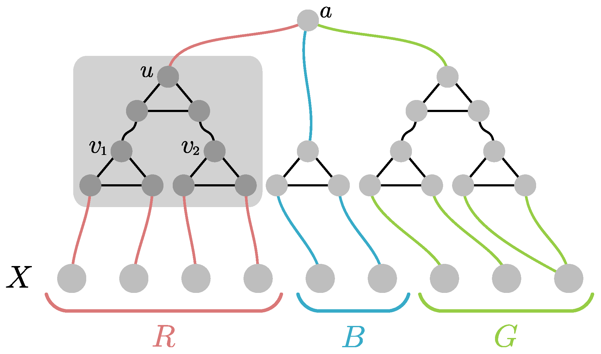
Proof. 

For any s we construct an s-Myhill–Nerode family $\mathcal{H}$. Let X be the s vertices in the boundary of all the boundaried graphs in the following. Then for every three-partition $\mathcal{X}=\{R,G,B\}$ of X we add a boundaried graph ${}^{\circ }{H}_{\mathcal{X}}$ to the family $\mathcal{H}$ by taking a single triangle $v_R,v_G,v_B$ and connecting the vertices $v_C$ to all vertices in $X\backslash C$ for $C\in \{R,G,B\}$. Notice that any 3-coloring of ${}^{\circ }{H}_{\mathcal{X}}$ induces the partition $\mathcal{X}$ on the nodes X. Since instances of three-coloring do not need any additional parameter, we ignore this part of the construction of $\mathcal{H}$ and implicitly assume that every graph in $\mathcal{H}$ is paired with zero.

To construct the graphs $G_{\mathcal{I}}$ for $\mathcal{I}\subset \mathcal{H}$, we will employ the circuit gadget $v_1,v_2,u$ highlighted in Figure 1. Please note that if $v_1,v_2$ receive the same color, then u must be necessarily colored the same. In every other case, the color of u is arbitrary. Now for every three-partition $\mathcal{X}=\{R,G,B\}$ of X we construct a testing gadget ${}^{\circ }{\mathsf{\Gamma }}_{\mathcal{X}}$ as follows: For every $C\in \{R,G,B\}$ we arbitrarily pair the vertices in C and connect them via the circuit gadget (as $v_1,v_2$). If $\left|C\right|$ is odd, we pair some vertex of C with itself. We then repeat the construction with all the u-vertices of those gadgets, resulting in a hierarchical structure of depth $\sim log\left|X\right|$ (c.f., Figure 1 for an example construction). Finally, we add a single vertex a and connect it to the top vertex of the three circuits. Please note that by the properties of the circuit gadget, the graph ${}^{\circ }{\mathsf{\Gamma }}_{\mathcal{X}}$ is three-colorable iff the coloring of X does not induce the partition $\mathcal{X}$. In particular, the graph ${}^{\circ }{\mathsf{\Gamma }}_{\mathcal{X}}\oplus {}^{\circ }{H}_{{\mathcal{X}}^{\prime }}$ is three-colorable iff $\mathcal{X}\ne {\mathcal{X}}^{\prime }$.

Now for every subset $\mathcal{I}\subseteq \mathcal{H}$ of graphs from the family, we define the graph ${}^{\circ }{G}_{\mathcal{I}}={⨁}_{{}^{\circ }{H}_{\mathcal{X}}\in \mathcal{I}}{}^{\circ }{\mathsf{\Gamma }}_{\mathcal{X}}$. By our previous observation, it follows that for every ${}^{\circ }{H}_{\mathcal{X}}\in \mathcal{H}$ the graph ${}^{\circ }{G}_{\mathcal{I}}\oplus {}^{\circ }{H}_{\mathcal{X}}$ is three-colorable iff ${}^{\circ }{H}_{\mathcal{X}}\notin \mathcal{I}$. Furthermore, every composite graph has treedepth at most $s+3\lceil logs\rceil +1$ as witnessed by a decomposition whose top s vertices are the boundary X and the rest has the structure of the graph itself after every triangle is made into a path. The graphs ${}^{\circ }{G}_{\mathcal{I}}$ for every $\mathcal{I}\subseteq \mathcal{H}$ have size at most $3^s·6s$. We conclude that $\mathcal{H}$ is an s-Myhill–Nerode family of size $3^s/6$ (the factor $1/6$ accounts for the $3!$ permutations of the partitions) and the claim follows from Lemma 1. ☐

Surprisingly, the construction to prove a lower bound for Vertex Cover is very similar to the one for 3-coloring.

Theorem 2.

For every $ϵ>0$, no DPTM solvesVertex Coveron a tree, path or treedepth decomposition of width/depth k with space bounded by $O({(2-ϵ)}^k·{log}^{O\left(1\right)}n)$.

Proof. 

For every s we construct an s-Myhill–Nerode family $\mathcal{H}$. Let X be the s vertices in the boundary of all the boundaried graphs in the following. Assume for now that s is even. For every subset $A\subseteq X$ such that $\left|A\right|=\left|X\right|/2$ we construct a graph ${}^{\circ }{H}_A$ which consists of the boundary as an independent set and a matching to A and add $({}^{\circ }{H}_A,s/2)$ to $\mathcal{H}$. Please note that any optimal vertex cover of any ${}^{\circ }{H}_A$ has size $s/2$ and that A is such a vertex cover.

Consider $\mathcal{I}\subseteq \mathcal{H}$. We will again use the circuit gadget highlighted in Figure 1 to construct ${}^{\circ }{G}_{\mathcal{I}}$. Please note that if either $v_1$ or $v_2$ is in the vertex cover we can cover the rest of gadget with two vertices, one of them being the top vertex u. Otherwise, u cannot be included in a vertex cover of size two. We still need two vertices, even if both $v_1$ and $v_2$ are already in the vertex cover. For a set $A\subseteq X$ such that $\left|A\right|=\left|X\right|/2$ we construct the testing gadget ${}^{\circ }{\mathsf{\Gamma }}_A$ by starting with the boundary X as an independent set, connecting the vertices of $X\backslash A$ pairwise via the circuit gadget (using an arbitrary pairing and potentially pairing a leftover vertex with itself). As in the proof of Theorem 1, we repeat this construction on the respective u-vertices of the circuits just added and iterate until we have added a single circuit at the very top. Let us denote the topmost u-vertex in this construction by $u^{\prime }$. Let $\lambda$ be the number of circuits added in this fashion. Any optimal vertex of ${}^{\circ }{\mathsf{\Gamma }}_A$ has size $2\lambda$ and does not include $u^{\prime }$. Please note that if a node of $X\backslash A$ is in the vertex cover, we can cover the rest of the gadget with $2\lambda$ many vertices, such that $u^{\prime }$ is part of the vertex cover.

We construct ${}^{\circ }{G}_{\mathcal{I}}$ by taking ${\oplus }_{{}^{\circ }{H}_A\in \mathcal{I}}{}^{\circ }{\mathsf{\Gamma }}_A$ and adding a single vertex a that connects to all $u^{\prime }$-vertices of the gadgets ${\{{}^{\circ }{\mathsf{\Gamma }}_A\}}_{{}^{\circ }{H}_A\in \mathcal{I}}$. Notice that, by the same reason $u^{\prime }$ was not part of an optimal vertex cover of any gadget ${}^{\circ }{\mathsf{\Gamma }}_A$, the node a must be part of any optimal vertex cover of ${}^{\circ }{G}_{\mathcal{I}}$ for $\left|\mathcal{I}\right|>1$. For $\left|\mathcal{I}\right|=1$ either the only $u^{\prime }$ or a must be contained besides the other vertices, but we will assume w.l.o.g that it is a. Let ℓ be the biggest optimal vertex cover for any such ${}^{\circ }{G}_{\mathcal{I}}$. Let ${\ell }_{\mathcal{I}}$ be the size of an optimal vertex cover for a specific ${}^{\circ }{G}_{\mathcal{I}}$. For simplicity, we pad ${}^{\circ }{G}_{\mathcal{I}}$ with $\ell -{\ell }_{\mathcal{I}}$ isolated $K_2$ subgraphs to ensure that the size of an optimal vertex cover is ℓ.

We claim that ${}^{\circ }{G}_{\mathcal{I}}\oplus {}^{\circ }{H}_A$ has a vertex cover of size $\ell +s/2-1$ iff ${}^{\circ }{H}_A\notin \mathcal{I}$. If $H_A\notin \mathcal{I}$, then for every gadget ${}^{\circ }{\mathsf{\Gamma }}_{A^{\prime }}$ that comprises ${}^{\circ }{G}_{\mathcal{I}}$ it holds that $A^{\prime }\ne A$. Since $|A^{\prime }|=|A|$ it follows that $(X\backslash A^{\prime })\cap A\ne \varnothing$. Since ${}^{\circ }{G}_{\mathcal{I}}\oplus {}^{\circ }{H}_A$ has $s/2$ vertices of degree one whose neighborhood is A, we can assume that an optimal vertex cover contains A. From the previous arguments about the possible vertex covers for the ${}^{\circ }{\mathsf{\Gamma }}_{A^{\prime }}$ gadgets it follows that the solution still needs two nodes for every circuit gadget of ${}^{\circ }{\mathsf{\Gamma }}_{A^{\prime }}$, but now this part of the vertex cover can include $u^{\prime }$. Since this is true for every ${}^{\circ }{\mathsf{\Gamma }}_{A^{\prime }}$ it follows that a does not need to be part of the vertex cover. Thus, the size of an optimal vertex cover is precisely $\ell +s/2-1$. If ${}^{\circ }{H}_A\in \mathcal{I}$ then the gadget ${}^{\circ }{\mathsf{\Gamma }}_A$ that has no vertex cover using two nodes per circuit gadget that contains its node $u^{\prime }$. It follows that any optimal vertex cover of ${}^{\circ }{G}_{\mathcal{I}}\oplus {}^{\circ }{H}_A$ must contain either a or its $u^{\prime }$. Thus the size of the solution is at least $\ell +s/2$. We thus set $p_{\mathcal{I}}$ to be $\ell -1$.

The size of the family $\mathcal{H}$ is, using Stirling’s approximation, bounded from below by

$$\left(\genfrac{}{}{0pt}{}{s}{s/2}\right)\ge \frac{2^{s-1}}{\sqrt{s/2}}$$

and is smaller than $2^s$. All numbers involved describe subsets of graphs and thus must be smaller than the sizes of those graphs. All graphs in the family have size s. The graphs ${}^{\circ }{G}_{\mathcal{I}}$ as described, are constructed by adding a polylogarithmic number of nodes to the boundary per gadget ${}^{\circ }{\mathsf{\Gamma }}_A$ and thus their size is bounded by $\left|\mathcal{H}\right|·{log}^{O\left(1\right)}\left|\mathcal{H}\right|$. For odd s we take $s^{\prime }=s-1$ and use the $s^{\prime }$-family as the s-family. The treedepth is $\mathbf{td}\left(\mathcal{H}\right)=s+o\left(s\right)$ by the same argument as for the construction for Theorem 1. We conclude that $\mathcal{H}$ is an s-Myhill–Nerode family of size $2^s/f\left(s\right)$ for $f\left(s\right)=s^{O\left(1\right)}\cap \mathsf{\Omega }\left(1\right)$ and depth $\mathbf{td}\left(\mathcal{H}\right)=s+o\left(s\right)$ and thus by Lemma 1 the theorem follows. ☐

Theorem 3.

For every $ϵ>0$, no DPTM solvesDominating Seton a tree, path or treedepth decomposition of width/depth k with space bounded by $O\left({(3-ϵ)}^k·{log}^{O\left(1\right)}n\right)$.

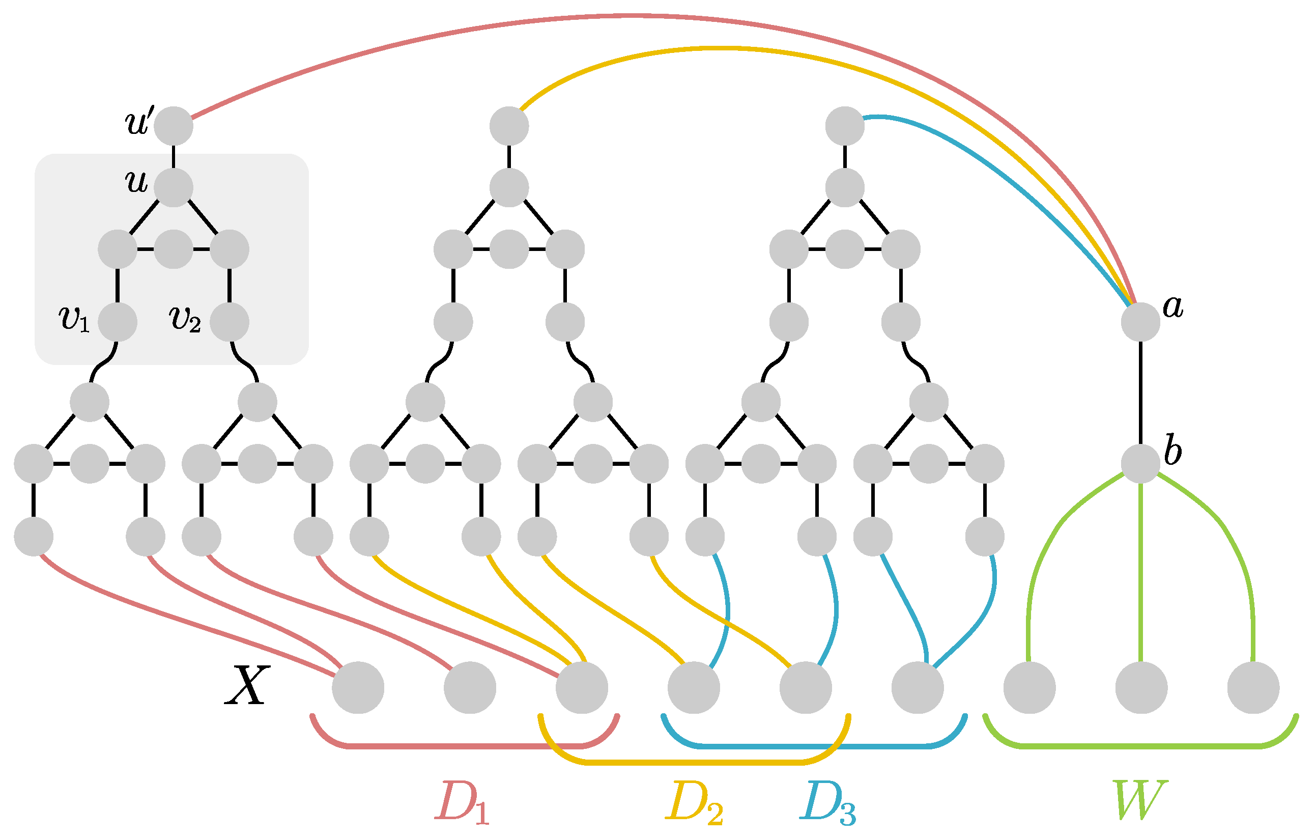
Proof. 

For any s divisible by three we construct an s-Myhill–Nerode family $\mathcal{H}$ as follows. Let X be the s boundary vertices of all the boundaried graphs in the following. Then for every three-partition $\mathcal{X}=(B,D,W)$ of X into sets of size $s/3$, we construct a graph $H_{\mathcal{X}}$ by connecting two new pendant vertices (with degree one) to every vertex in B, connecting every vertex in D to a vertex which itself is connected to two pendant vertices and leaving W untouched and thus isolated. Intuitively, we want the vertices of B to be in any minimal dominating set, the vertices in D to be dominated from a vertex in $H_{\mathcal{X}}$ not in the boundary and the vertices in W to be dominated from elsewhere. We add every pair $(H_{\mathcal{X}},2s/3)$ to $\mathcal{H}$. Notice that the size of an optimal dominating set of $H_{\mathcal{X}}[B\cup D]$ is $2s/3$ and there is only one such optimal dominating set, namely $B\cup N\left(D\right)$.

For a subset $\mathcal{I}\subseteq \mathcal{H}$ let ${\mathcal{D}}_W=\{D\mid H_{(X\backslash (D\cup W),D,W)}\in \mathcal{I}\}$ be a set defined for every $W\subset X$. We construct the graph ${}^{\circ }{G}_{\mathcal{I}}$ using the circuit gadget with nodes $v_1,v_2,u$ highlighted in Figure 2: Please note that if $v_1,v_2$ need to be dominated, then there is no dominating set of the gadget of size two that contains u. If one of $v_1,v_2$ does not need to be dominated (but is not in the dominating set) then a dominating set of size two of the circuit gadget containing u exists. For every $W\subset X$ with $\left|W\right|=s/3$ construct a testing gadget ${}^{\circ }{\mathsf{\Gamma }}_W$ as follows. Assume first that ${\mathcal{D}}_W$ is non-empty. For every set $D\in {\mathcal{D}}_W$ we construct the gadget ${}^{\circ }{\mathsf{\Lambda }}_D$ by arbitrarily pairing the vertices in D and connecting them via the circuit gadget as exemplified in Figure 2. This closely parallels the constructions we have seen in the proofs for Theorem 1 and 2: If $\left|D\right|$ is odd, we pair some vertex of D with itself. We then repeat the construction with all the u-vertices of those gadgets, resulting in a hierarchical structure of depth $\sim log\left|D\right|$. To finalize the construction of ${}^{\circ }{\mathsf{\Lambda }}_D$ we take the u-vertex of the last layer and connect it to a new vertex $u^{\prime }$. This concludes the construction of ${}^{\circ }{\mathsf{\Lambda }}_D$. Let in the following $\lambda$ be the number of circuits we used to construct such a ${}^{\circ }{\mathsf{\Lambda }}_D$ gadget (this quantity only depends on s and is the same for any ${}^{\circ }{\mathsf{\Lambda }}_D$). If ${\mathcal{D}}_W$ is empty, then ${}^{\circ }{\mathsf{\Gamma }}_W$ is the boundary and a $K_2$ with one of its vertices connected to all vertices in W plus $\left(\genfrac{}{}{0pt}{}{2s/3}{s/3}\right)2\lambda$ isolated padding-vertices. Otherwise we obtain ${}^{\circ }{\mathsf{\Gamma }}_W$ by taking the graph ${⨁}_{D\in \mathcal{D}}{}^{\circ }{\mathsf{\Lambda }}_D$ and adding two additional vertices $a,b$ as well as $\left(\left(\genfrac{}{}{0pt}{}{2s/3}{s/3}\right)-\left|{\mathcal{D}}_W\right|\right)2\lambda$ isolated vertices for padding. The vertex a is connected to all $u^{\prime }$ vertices of all the gadgets ${\{{}^{\circ }{\mathsf{\Lambda }}_D\}}_{D\in {\mathcal{D}}_W}$ and the vertex b is connected to $\{a\}\cup W$ (c.f., again Figure 2 for an example). Finally we define for every $\mathcal{I}\subseteq \mathcal{H}$ the graph ${}^{\circ }{G}_{\mathcal{I}}={⨁}_{W\subset X,\left|W\right|=s/3}{}^{\circ }{\mathsf{\Gamma }}_W$.

Let $\alpha =\left(\genfrac{}{}{0pt}{}{2s/3}{s/3}\right)2\lambda +1$. Consider some ${}^{\circ }{\mathsf{\Gamma }}_W$, for a W such that ${\mathcal{D}}_W\ne \varnothing$. Assume we start with a dominating set S such that $S\cap D=\varnothing$ for at least one $D\in D_W$. We want to show that extending S to dominate $V(({}^{\circ }{\mathsf{\Gamma }}_W)\backslash X)\cup W$ requires at least $\alpha +1$ many vertices. We can assume that b must be added to the dominating set. All $\left(\left(\genfrac{}{}{0pt}{}{2s/3}{s/3}\right)-\left|{\mathcal{D}}_W\right|\right)2\lambda$ padding vertices must also be added. Since we need at least two vertices per circuit gadget, at least $2\lambda$ vertices will always be necessary to dominate each ${}^{\circ }{\mathsf{\Lambda }}_D$ subgraph of ${}^{\circ }{\mathsf{\Gamma }}_W$ (of which there are $|{\mathcal{D}}_W|$ many). For ${}^{\circ }{\mathsf{\Lambda }}_D$ where $S\cap D=\varnothing$ no dominating set of the circuit gadgets of size $2\lambda$ can also dominate $u^{\prime }$. Thus we also need to take a or $u^{\prime }$ into the dominating set and we need at least $\alpha +1$ many vertices.

Now assume that we start with a dominating set S that contains at least one node of every $D\in {\mathcal{D}}_W\ne \varnothing$. In this case we can dominate all the circuit gadgets and $u^{\prime }$ with $2\lambda$ many nodes in every ${}^{\circ }{\mathsf{\Lambda }}_D$. Thus, there is a set in ${}^{\circ }{\mathsf{\Gamma }}_W$ that dominates $V(({}^{\circ }{\mathsf{\Gamma }}_W)\backslash X)\cup W$ of size $\alpha$, since neither a nor any $u^{\prime }$ needs to be in the dominating set.

Let us now show that our boundaried graphs work as intended and calculate the appropriate parameters $p_{\mathcal{I}}$. Consider any graph ${}^{\circ }{H}_{(B_0,D_0,W_0)}\in \mathcal{H}$ and the graph ${}^{\circ }{G}_{\mathcal{I}}$ for any $\mathcal{I}\subseteq \mathcal{H}$. We show that ${}^{\circ }{H}_{(B_0,D_0,W_0)}\oplus G_{\mathcal{I}}$ has an optimal dominating set of size at most $\left(\genfrac{}{}{0pt}{}{s}{s/3}\right)\alpha +2s/3$ iff ${}^{\circ }{H}_{(B_0,D_0,W_0)}\notin \mathcal{I}$. We need to include the $s/3$ vertices of $B_0$ and the $s/3$ vertices of $N(D)\cap V({}^{\circ }{H}_{(B_0,D_0,W_0)})$. We use the sets ${\mathcal{D}}_W$ as defined previously. First, assume that ${\mathcal{D}}_{W_0}=\varnothing$, that is, for every set $B^{\prime },D^{\prime }$ we have that $H_{(B^{\prime },D^{\prime },W_0)}\notin \mathcal{I}$ and in particular $H_{(B_0,D_0,W_0)}\notin \mathcal{I}$. It is easy to see that the simple version of the gadget ${}^{\circ }{\mathsf{\Gamma }}_{W_0}$ for the case where ${\mathcal{D}}_{W_0}=\varnothing$ can dominate its non-boundary nodes and $W_0$ with $\alpha$ nodes. All other gadgets ${}^{\circ }{\mathsf{\Gamma }}_{W^{\prime }}$ for $W^{\prime }\ne W_0$ do not need to dominate their respective $W^{\prime }$-sets and can therefore include their a-vertices and not include their b-vertices. Accordingly, they can all dominate their internal vertices with $\alpha$ many nodes. This all adds up to a dominating set of size $\left(\genfrac{}{}{0pt}{}{s}{s/3}\right)\alpha +2s/3$. Next, assume that ${\mathcal{D}}_{W_0}\ne \varnothing$ and $D_0\notin {\mathcal{D}}_{W_0}$, i.e., again $H_{(B_0,D_0,W_0)}\notin \mathcal{I}$. Therefore, for every set $D^{\prime }\in D_{W_0}$ we have that $D^{\prime }\cap B_0\ne \varnothing$. Since we can assume $B_0$ is part of our dominating set, we only need to add $\alpha$ vertices to the dominating from ${}^{\circ }{\mathsf{\Gamma }}_{W_0}$ to dominate $V(({}^{\circ }{\mathsf{\Gamma }}_{W_0})\backslash X)\cup W_0$. All gadgets ${}^{\circ }{\mathsf{\Gamma }}_{W^{\prime }},W^{\prime }\ne W_0$ also need $\alpha$ vertices, as observed above. We obtain in total a dominating set of size $\left(\genfrac{}{}{0pt}{}{s}{s/3}\right)\alpha +2s/3$. Finally, consider the case that $D_0\in {\mathcal{D}}_{W_0}$, i.e., $H_{(B_0,D_0,W_0)}\in \mathcal{I}$. Since $B_0\cap D_0=\varnothing$ the gadget ${}^{\circ }{\mathsf{\Lambda }}_{D_0}$ needs $\alpha +1$ vertices to dominate $V(({}^{\circ }{\mathsf{\Gamma }}_{W_0})\backslash X)\cup W_0$. Dominating $W_0$ with nodes different from the b-vertex of ${}^{\circ }{\mathsf{\Gamma }}_{W_0}$ does not help. Thus, we need at least $\left(\genfrac{}{}{0pt}{}{s}{s/3}\right)\alpha +2s/3+1$ vertices to dominate ${}^{\circ }{H}_{(B_0,D_0,W_0)}\oplus G_{\mathcal{I}}$.

Choosing $p_{\mathcal{I}}=\left(\genfrac{}{}{0pt}{}{s}{s/3}\right)\alpha$ completes the construction of $({}^{\circ }{G}_{\mathcal{I}},p_{\mathcal{I}})$. The size of all these graphs is bounded by $O(\left(\genfrac{}{}{0pt}{}{s}{s/3}\right)\left(\genfrac{}{}{0pt}{}{2s/3}{s/3}\right)logs)=O(3^{s}logs)$. We conclude that $\mathcal{H}$ is an s-Myhill–Nerode family of size $\left(\genfrac{}{}{0pt}{}{s}{s/3}\right)\left(\genfrac{}{}{0pt}{}{2s/3}{s/3}\right)$ which is $\mathsf{\Omega }(3^s/s)$ and $O(3^s)$. For s indivisible by three we take the next smaller integer $s^{\prime }$ divisible by three and use $s^{\prime }$-family as the s-family. It is easy to confirm that the treedepth of $\mathcal{H}$ is $\mathbf{td}\left(\mathcal{H}\right)=s+o\left(s\right)$ and the theorem follows from Lemma 1. ☐

5. Dominating Set Using $\mathit{O}({\mathit{d}}^{\mathbf{3}}log\mathit{d}+\mathit{d}log\mathit{n})$ Space

That branching might be a viable algorithmic design strategy for low-treedepth graphs can easily be demonstrated for problems like 3-Coloring and Vertex Cover: We simply branch on the topmost vertex of the decomposition and recur into (annotated) subinstances. For q-Coloring, this leads to an algorithm with running time $O(q^d·n)$ and space complexity $O(dlogn)$. Since it is possible to perform a depth-first traversal of a given tree using only $O(logn)$ space [38], the space consumption of this algorithm can be easily improved to $O(d+logn)$. Similarly, branching solves Vertex Cover in time $O(2^d·n)$ and space $O(dlogn)$.

The task of designing a similar algorithm for Dominating Set is much more involved. Imagine branching on the topmost vertex of the decomposition: while the branch that includes the vertex into the dominating set produces a straightforward recurrence into annotated instances, the branch that excludes it from the dominating set needs to decide how that vertex should be dominated. The algorithm we present here proceeds as follows: We first guess whether the current node x is in the dominating set or not. Recall that $P_x$ denotes the nodes of the decomposition that lie on the unique path from x to the root of the decomposition (and $x\notin P_x$). We iterate over every possible partition $S_1\uplus \cdots \uplus S_{\ell }=P_x\cup \{x\}$ into $\ell \le d$ sets of $P_x\cup \{x\}$. The semantic of a block $S_i$ is that we want every element $S_i$ to be dominated exclusively by nodes from a specific subtree of x. A recursive call on a child y of x, together with an element of the partition $S_i$, will return the size of a dominating set which dominates $V(T_y)\cup S_i$. The remaining issue is how these specific solutions for the subtrees of x can be combined into a solution in a space-efficient manner. To that end, we first compute the size of a dominating set for $T_y$ itself and use this as baseline cost for a subtree $T_y$. For a block $S_i$ of a partition of $P_x$, we can now compare the cost of dominating $V(T_y)\cup S_i$ against this baseline to obtain overhead cost of dominating $S_i$ using vertices from $T_y$. Collecting these overhead costs in a table for subtrees of x and the current partition, we are able to apply certain reduction rules on these tables to reduce their size to at most $d^2$ entries. Recursively choosing the best partition then yields the solution size using only polynomial space in d and logarithmic in n. Formally, we prove the following:

Theorem 4.

Given a graph G and a treedepth decomposition T of G, Algorithm 1 finds the size of a minimum dominating set of G in time $d^{O(d^2)}·n$ using $O(d^{3}logd+dlogn)$ bits.

We split the proof of Theorem 4 into lemmas for correctness, running time and used space.

Lemma 2.

Algorithm 1 called on a graph G, a treedepth decomposition T of G, the root r of T and $P=D=\varnothing$ returns the size of a minimum dominating set of G.

Proof. 

If we look at a minimal dominating set S of G we can charge every node in $V\left(G\right)\backslash S$ to a node from S that dominates it. We are thus allowed to treat any node in G as if it was dominated by a single node of S. We will prove this lemma by induction, the inductive hypothesis being that a call on a node x with arguments $D=S\cap P_x$ and $P\subseteq P_x$ being the set of nodes dominated from nodes in $T_x$ by S returns $|S\cap V(T_x)|$.

It is clear that the algorithm will call itself until a leaf is reached. Let x be a leaf of T on which the function was called. We first check the condition at line 2, which is true if either x is not dominated by a node in D or if some node in P is not yet dominated. In this case we have no choice but to add x to the dominating set. Three things can happen: P is not fully dominated, which means that it was not possible under these conditions to dominate P, in which case we correctly return ∞, signifying that there is no valid solution. Otherwise we can assume P is dominated and we return 1 if we had to take x and 0 if we did not need to do so. Thus, the leaf case is correct.

We assume now x is not a leaf and thus we reach line 7. We first add x to P, since it can only be dominated either from a node in D or a node in $T_x$. Nodes in $T_x$ can only be dominated by nodes from $V\left(T_x\right)\cup P_x$. We assume by induction that $D=S\cap P_x$ and that P only contains nodes which are either in S or dominated from nodes in $T_x$. Algorithm 1 executes the same computations for D and $D\cup \{x\}$, representing not taking and taking x into the dominating set respectively. We must show that the set P for the recursive calls is correct. There exists a partition of the nodes of P not dominated by D (respectively $D\cup \{x\}$) such that the nodes of every element of the partition are dominated from a single subtree $T_y$ where y is a child of x. The algorithm will eventually find this partition on line 9. The baseline value, i.e., the size of a dominating set of $T_y$ given that the nodes in D (respectively $D\cup \{x\}$) are in the dominating set, gives a lower bound for any solution. In the lists in L and $L^{\prime }$ we keep the extra cost incurred by a subtree $T_y$ if it has to dominate an element of the partition. We only need to keep the best d values for every $S_i$: Assume that it is optimal to dominate $S_i$ from $T_y$ and there are $d+1$ subtrees induced on children $y^{\prime }\ne y$ of x whose extra cost over the baseline to dominate $S_i$ is strictly smaller than the extra cost for $T_y$. At least one of these subtrees $T_{y^{\prime }}$ is not being used to dominate an element of the partition. This means we could improve the solution by letting $T_y$ dominate itself and taking the solution of $T_{y^{\prime }}$ that also dominates $S_i$. Keeping d values for every element in the partition suffices to find a minimal solution, which is what find_min_solution $\left(L\right)$ does as follows: Create a bipartite graph $G=(A\uplus B,E)$ such that A contains a node for every $S_i$ and B contains a node for every y for which there is an entry $(·,y)$ in L. For every node a representing $S_i$ we add an edge with weight $d-c$ to a node b representing y if $(c,y)\in L[i]$. Notice that the minimal number of nodes above the baseline needed to dominate an element of the partition is always less than d. A maximal matching in this bipartite graph tells us how many nodes above the baseline are required to dominate the elements of the partition from subtrees rooted at children of x. Since L contains at most $d^2$ entries this can be computed in polynomial time in d. Since with lines 27 and 28 we take the minimum over all possible partitions and taking x into the dominating set or not, we get that by inductive assumption the algorithm returns the correct value. The lemma follows since the first call to the algorithm with $D=P=\varnothing$ is obviously correct. ☐

Lemma 3.

Algorithm 1 runs in time $d^{O(d^2)}·n$.

Proof. 

The running time when x is a leaf is bounded by $O(d^2)$, since all operations exclusively involve some subset of the d nodes in $P_x\cup \{x\}$. Since $\left|P\right|\le d$ the number of partitions of P is bounded by $d^d$. When x is not a leaf the only time spent on computations which are not recursive calls of the algorithm are all trivially bounded by $O\left(d\right)$, except the time spent on find_min_solution, which can be solved via a matching problem in polynomial time in d (see proof of Lemma 2). The number of recursive calls that a single call on a node x makes on a child y is $O(d·d^d)$ which bounds the total number of calls on a single node by $d^{O(d^2)}$. This proves the claim. ☐

Lemma 4.

Algorithm 1 uses $O(d^{3}logd+dlogn)$ bits of space.

Proof. 

There are at most d recursive calls on the stack at any point. We will show that the space used by one is bounded by $O(d^{2}logd+logn)$. Each call uses $O\left(d\right)$ sets, all of which have size at most d. The elements contained in these sets can be represented by their position in the path to the root of T, thus they use at most $O(d^{2}logd)$ space. The arrays of ordered lists $L,L^{\prime }$ contain at most $d^2$ elements and all entries are ≤d or ∞: If the additional cost (compared to the baseline cost) of dominating a block $S_i$ of the current partition from some subtree $T_y$ exceeds d, we disregard this possibility—it would be cheaper to just take all vertices in $S_i$, a possibility explored in a different branch. To find a minimal solution from the table we need to avoid using the same subtree to dominate more than one element of the partition; however, at any given moment we only need to distinguish at most $d^2$ subtrees. Thus, the size of the arrays L and $L^{\prime }$ is bounded by $O(d^{2}logd)$. The only other space consumption is caused by a constant number of variables (result, baseline, ${\mathit{baseline}}^{\prime }$, b, $b^{\prime }$ and x) all of them $\le n$. Thus, the space consumption of a single call is bounded by $O(d^{2}logd+logn)$ and the lemma follows. ☐

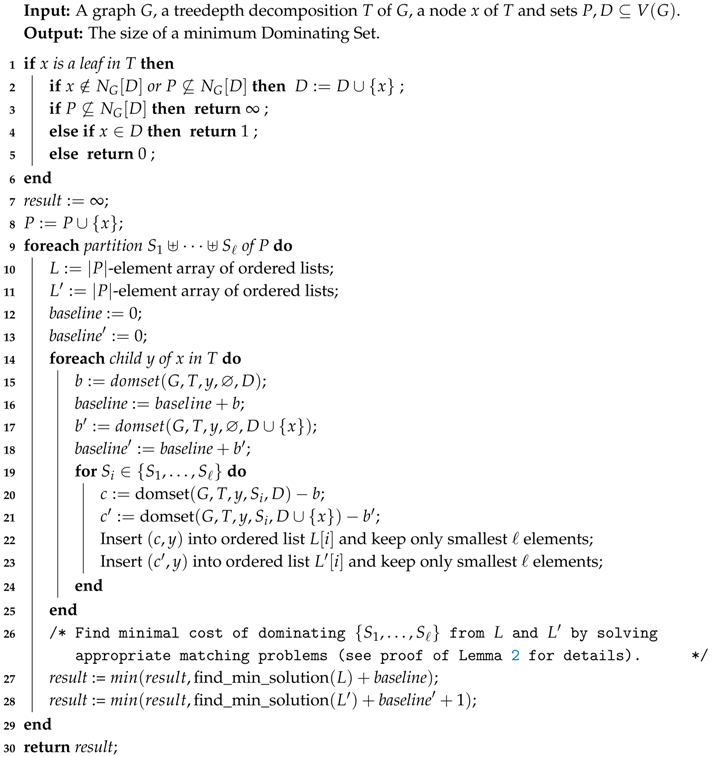
Algorithm 1: Computing dominating sets with very little space.

6. Fast Dominating Set Using $\mathit{O}({\mathbf{2}}^{\mathit{d}}\mathit{d}log\mathit{d}+\mathit{d}log\mathit{n})$ Space

We have seen that it is possible to solve Dominating Set on low-treedepth graphs in a space-efficient manner. However, we traded space exponential in the treedepth against superexponential running time in the treedepth and it is natural to ask whether there is some middle ground. We present Algorithm 2 to answer this question: its running time $O(3^{d}logd·n)$ is competitive with the default dynamic programming but its space complexity $O(2^{d}logd+dlogn)$ is exponentially better. The basic idea is to again branch from the top deciding if the current node x is in the dominating set or not. Intertwined in this branching we compute a function which for a subtree $T_x$ and a set $S\subseteq P_x$ gives the cost of dominating $V(T_x)\cup S$ from $T_x$. For each recursive call on a node we only need this function for subsets of $P_x$ which are not dominated. If $d^{\prime }$ is the number of nodes of $P_x$ that are currently contained in D, the function only needs to be computed for $2^{d-d^{\prime }}$ sets. This allows us to keep the running time of $O^{\ast }(3^d)$, since ${\sum }_{i=0}^d\left(\genfrac{}{}{0pt}{}{d}{i}\right)·2^{d-i}=3^d$, while only creating tables with at most $O(2^d)$ entries. By representing all values in these tables as $\le d$ offsets from a base value, the space bound $O(2^{d}dlogd+dlogn)$ follows. Part of the algorithm will be convolution operations.

Definition 4 (Convolution).

For two functions $M_1,M_2$ with domain $2^U$ for some ground-set U we use the notation $M_1\ast M_2$ to denote the convolution $(M_1\ast M_2)\left[X\right]:={min}_{A\uplus B=X}{M}_1\left[A\right]+M_2\left[B\right],$ for all $X\subseteq U$.

Algorithm 2: Computing dominating sets with $O^{\ast }(2^d)$ space.

Theorem 5.

For a graph G with treedepth decomposition T, Algorithm 2 finds the size of a minimum dominating set in time $O(3^{d}logd·n)$ using $O(2^{d}dlogd+dlogn)$ bits of space.

We divide the proof into lemmas as before.

Lemma 5.

Algorithm 2 called on $G,T,r,\varnothing$, where T is a treedepth decomposition of G with root r, returns the size of a minimum dominating set of G.

Proof. 

Notice that the associative array M represents a function which maps subsets of $P_x\backslash D$ to integers and ∞. At the end of any recursive call, $M\left[S\right]$ for $S\subseteq P_x\backslash D$ should be the size of a minimal dominating set in $T_x$ which dominates $T_x$ and S assuming that the nodes in D are part of the dominating set. We will prove this inductively.

Assume x is a leaf. We can always take x into the dominating set at cost one. In case x is already dominated we have the option of not taking it, dominating nothing at zero cost. This is exactly what is computed in lines 2–5.

Assume now that x is an internal, non-root node of T. First, in lines 8–13 we assume that x is not in the dominating set. By inductive assumption calling $domset$ on a child y of x returns a table which contains the cost of dominating $T_y$ and some set $S\subseteq P_y\backslash D$. By convoluting them all together $M_1$ represents a function which gives the cost of dominating some set $S\subseteq (P_x\cup \{x\})\backslash D$ and all subtrees rooted at children of x. We just need to take care that x is dominated. If x is not dominated by a node in D, then it must be dominated from one of the subtrees. Thus, we are only allowed to retain solutions which dominate x from the subtrees. We take care of this on line 13. After this $M_1$ represents a function which gives the cost of dominating some set $S\subseteq (P_x\cup \{x\})\backslash D$ and $T_x$ assuming x is not in the dominating set. Then we compute a solution assuming x is in the dominating set in lines 14–18. We first merge the results on calls to the children of x via convolution. Since we took x into the dominating set we increase the cost of all entries by one. After this $M_2$ represents the function which gives the cost of dominating some set $S\subseteq P_x\backslash D$ and $T_x$ assuming x is in the dominating set. We finally merge $M_1$ and $M_2$ by taking the minimums. Since we have taken care that all solutions represented by entries in M dominate x we can remove all information about x. We do this in lines 21–22. Finally, M represents the desired function and we return it. When x is the root, instead of returning the table we return the value for the only entry in M, which is precisely the size of a minimum dominating set of G. ☐

To prove the running time of Algorithm 2 we will need the values M to be all smaller or equal to the depth of T. Thus, we first prove the space upper bound. In the following we treat the associative arrays M, $M_1$ and $M_2$ as if the entries where values between 0 and n. We will show that we can represent all values as an offset $\le d$ of a single single value between 0 and n.

Lemma 6.

Algorithm 2 uses $O(2^{d}dlogd+dlogn)$ bits of space.

Proof. 

Let d be the depth of the provided treedepth decomposition. It is clear that the depth of the recursion is at most d. Any call to the function keeps a constant number of associative arrays and nodes of the graph in memory. By construction these associative arrays have at most $2^d$ entries. For any of the computed arrays M the value of $M[\varnothing ]$ and $M[S]$ for any $S\ne \varnothing$ can only differ by at most d. We can thus represent every entry for such a set S as an offset from $M[\varnothing ]$ and use $O(2^{d}logd+logn)$ space for the tables. This together with the bound on the recursion depth gives the bound $O(2^{d}dlogd+dlogn)$. ☐

Lemma 7.

Algorithm 2 runs in time $O(3^{d}logd·n)$.

Proof. 

On a call on which $d^{\prime }$ nodes of $P_x$ are in the dominating set the associative arrays have at most $2^s$ entries for $s=d-d^{\prime }$. As shown above the entries in the arrays are $\le s$ (except one). Hence, we can use fast subset convolution to merge the arrays in time $O(2^{s}logs)$ [39]. It follows that the total running time is bounded by

$$O\left(n·\sum _{i=0}^d\left(\genfrac{}{}{0pt}{}{d}{i}\right)·2^{d-i}log(d-i)\right)=O(3^{d}logd·n)$$

and thus the lemma follows. ☐

7. Conclusions and Future Work

We have shown that single-pass dynamic programming algorithms on treedepth, tree or path decompositions without preprocessing of the input must use space exponential in the width/depth, confirming a common suspicion and proving it rigorously for the first time. This complements previous SETH-based arguments about the running time of arbitrary algorithms on low treewidth graphs. We further demonstrate that treedepth allows non-DP linear-time algorithms that only use polynomial space in the depth of the provided decomposition. Both our lower bounds and the provided algorithm for Dominating Set appear as if they could be special cases of a general theory to be developed in future work and we further ask whether our result can be extended to less stringent definitions of “dynamic programming algorithms”.

It would be great to be able to characterize exactly which problems can be solved in linear-fpt time using $\mathrm{poly}(d)·logn$ space. Tobias Oelschlägel proved as part of his master thesis [40] that the ideas presented here can be extended to the framework of Telle and Proskurowski for graph partitioning problems [41]. Mimicking the development for treewidth would point to extending this result to MSO. Sadly, a proven double exponential dependency on the run-time of model-checking MSO parameterized by the size of a vertex cover implies that no such result is possible [42]. Is there a characterization that better captures for which problems this is possible? Previous research that might be relevant to this endeavor has investigated the height of the tower in the running time for MSO model-checking on graphs of bounded treedepth [43].

Despite the less-than-ideal theoretical bounds of the presented Dominating Set algorithms, the opportunities for heuristic improvements are not to be slighted. Take the pure branching algorithm presented in Section 5. During the branching procedure, we generate all partitions from the root-path starting at the current vertex. However, we actually only have to partition those vertices that are not dominated yet (by virtue of being themselves in the dominating set or being dominated by another vertex on the root-path). A sensible heuristic as to which branch—including the current vertex in the dominating set or not—to explore first, together with a branch and bound routine should keep us from generating partitions of very large sets. A similar logic applies to the mixed dynamic programming/branching algorithm since the tables only have to contain information about sets that are not yet dominated. It might thus be possible to keep the tables a lot smaller than their theoretical bounds indicate.

Furthermore, it seems reasonable that in practical settings, the nodes near the root of treedepth decompositions are more likely to be part of a minimal dominating set. If this is true, computing a treedepth decomposition would serve as a form of smart preprocessing for the branching, a rough “plan of attack”, if you will. How much such a guided branching improves upon known branching algorithms in practice is an interesting avenue for further research.

It is still an open question, proposed by Michał Pilipczuk during GROW 2015, whether Dominating Set can be solved in time ${(3-ϵ)}^d·\mathrm{poly}\left(n\right)$ when parameterized by treedepth. Our lower bound result implies that if such an algorithm exists, it cannot be a straightforward dynamic programming algorithm.