1. Introduction
A string is a sequence of symbols from an alphabet
, in which a symbol can be repeated. An
adjacent swap exchanges two consecutive elements in a sequence [
1,
2]. In a
signed string (
,
) the following signs are assigned: + for normal orientation and − for reverse orientation. Adjacent swap over positions
are denoted by (
). For unsigned strings (
), where
=
,
transforms into
, where
=
. For signed strings (
), where
=
,
transforms into
, where
=
. Two strings are
compatible under some operation if they can be transformed into each other with the operation. That is, the unsigned string (2, 1, 3, 2) is compatible with (2, 1, 2, 3), whereas it is not compatible with (3, 2, 1, 1). The computation of the minimum number of adjacent swaps required to transform one given string into another compatible string, i.e., the
adjacent swap distance, has applications in genetics and music theory [
1]. A 1-
flip toggles the orientation of a particular
; it is denoted by
. It changes the sign of
. When it is applied to a signed string (
), where
=
,
transforms into
, where
=
.
A
short reversal is either a (1-
flip) or an adjacent swap. The
short reversal distance is the minimum number of short reversals required to transform a signed string into another compatible string. Two strings are compatible under short reversals if and only if their unsigned versions, i.e., the strings whose signs are disregarded, are compatible [
1]. The computation of the short reversal distance between
and
is reduced to the computation of the cardinality of the maximum independent set on a conflict graph constructed from
and
. It has applications in HOX gene clusters in vertebrate evolution [
2,
3]. In music theory, a composition is represented as a string. The smaller the distance between two patterns (compositions), the more similar they are [
4].
The maximum independent set problem on a graph,
, seeks to identify a subset of
V with maximum cardinality, such that no two vertices in the subset have an edge between them. If
is the maximum independent set (or MIS for short) of
G, then
. In this article,
G is undirected, so an edge
is understood to be an undirected edge. Karp proposed a method for proving problems to be NP-complete [
5]. The maximum independent set problem on a general graph is known to be NP-complete [
6]. Certain classes of graphs have a polynomial time solution for this problem. Such algorithms are known for trees and bipartite graphs [
7], chordal graphs [
8], cycle graphs [
9], comparability graphs [
10], claw-free graphs [
11], interval graphs and circular arc graphs [
12]. The maximum weight independent set problem is defined on a graph where the vertices are mapped to corresponding weights. The maximum weight independent set problem seeks to identify an independent set where the sum of the weights of the vertices is maximized. On trees, the maximum weighted independent set problem can be solved in linear time [
13]. Thus, for several classes of graphs, MIS can be efficiently computed.
Hsiao et al. designed an
time algorithm to solve the maximum weight independent set problem on an interval graph with
n vertices, given its interval representation with a sorted endpoints list [
14]. Several articles improved the complexity of the exponential algorithms that compute an MIS on a general graph [
15,
16]. Lozin and Milanic showed that MIS is polynomially solvable for the class of
-free planar graphs, generalizing several previously known results, where
is the graph consisting of three induced paths of lengths 1, 2 and
k with a common initial vertex [
17].
The minimum vertex cover problem on
G seeks to identify a vertex cover with minimum cardinality, i.e., minimum vertex cover or MVC. If
is the MVC of
G, then
,
. In this article,
G is undirected, so an edge
is understood to be an undirected edge. The minimum dominating set (i.e., MDS) and the minimum connected dominating set (i.e., MCD) problems seek to identify a dominating set i.e., DS and a connected dominating set i.e., CDS, respectively, with minimum cardinalities. The MVC, MDS and MCD problems on general graphs are known to be NP-complete [
6]. Garey and Johnson showed that MVC is one of the first NP-complete problems [
6]. In connected vertex cover problems (i.e., MCV), given a connected graph (G), a connected vertex cover (i.e., CVC) with minimum cardinality is sought. Garey and Johnson proved that MCV is NP-complete [
18]. For trees and bipartite graphs, the minimum vertex cover can be identified in polynomial time [
19,
20]. Garey and Johnson proved that the MCV problem is NP-hard in planar graphs, with a maximum degree of 4 [
6]. Li et al. proved that for 4-regular graphs, the MCV problem is NP-hard [
21]. It has been shown that for series-parallel graphs, which are a set of planar graphs, the minimum vertex cover can be computed in linear time [
22].
Garey and Johnson showed that the MDS problems on planar graphs with maximum vertex degree 3 and planar graphs that are regular with degree 4 are NP-complete [
6]. MCD is NP-complete even for planar graphs that are regular with degree 4 [
6]. Bertossi showed that the problem of identifying a MDS is NP-complete for split graphs and bipartite graphs [
23]. Cockayne et al. proved that MDS in trees can be computed in linear time [
24]. Baker designed various approximation algorithms for planar graphs [
25]. Muller and Brandstadt showed that MDS and MCD are NP-complete for chordal bipartite graphs [
26]. Ruo-Wei et al. proved that for a given circular arc graph with
n sorted arcs, MCD is linear in time and space [
27]. Fomin et al. proposed an algorithm with a time complexity faster than
to solve the connected dominating set problem [
28].
The term “layered graph” has been used in the literature. The hop-constrained minimum spanning tree problem related to the design of centralized telecommunication networks with quality of service (QoS) constraints is NP-hard [
29]. A graph known as a
layered graph was constructed from a given input graph, and the authors showed that the hop-constrained minimum spanning tree problem is equivalent to the Steiner tree problem. In software architecture, the system is divided into several layers; this has been viewed as a graph with several layers. In this article, we define a new class of graphs that we call
layered graphs and design algorithms for various graph-theoretic problems.
2. Layered Graph
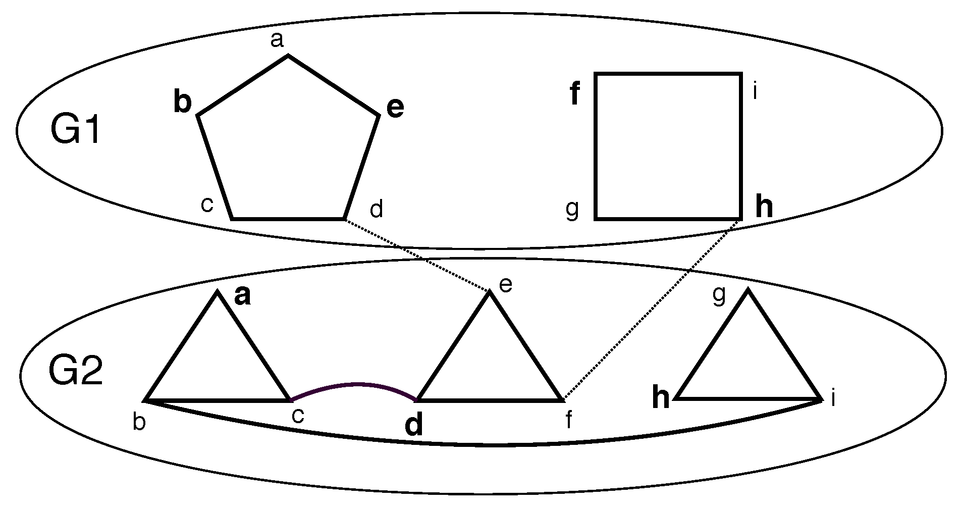
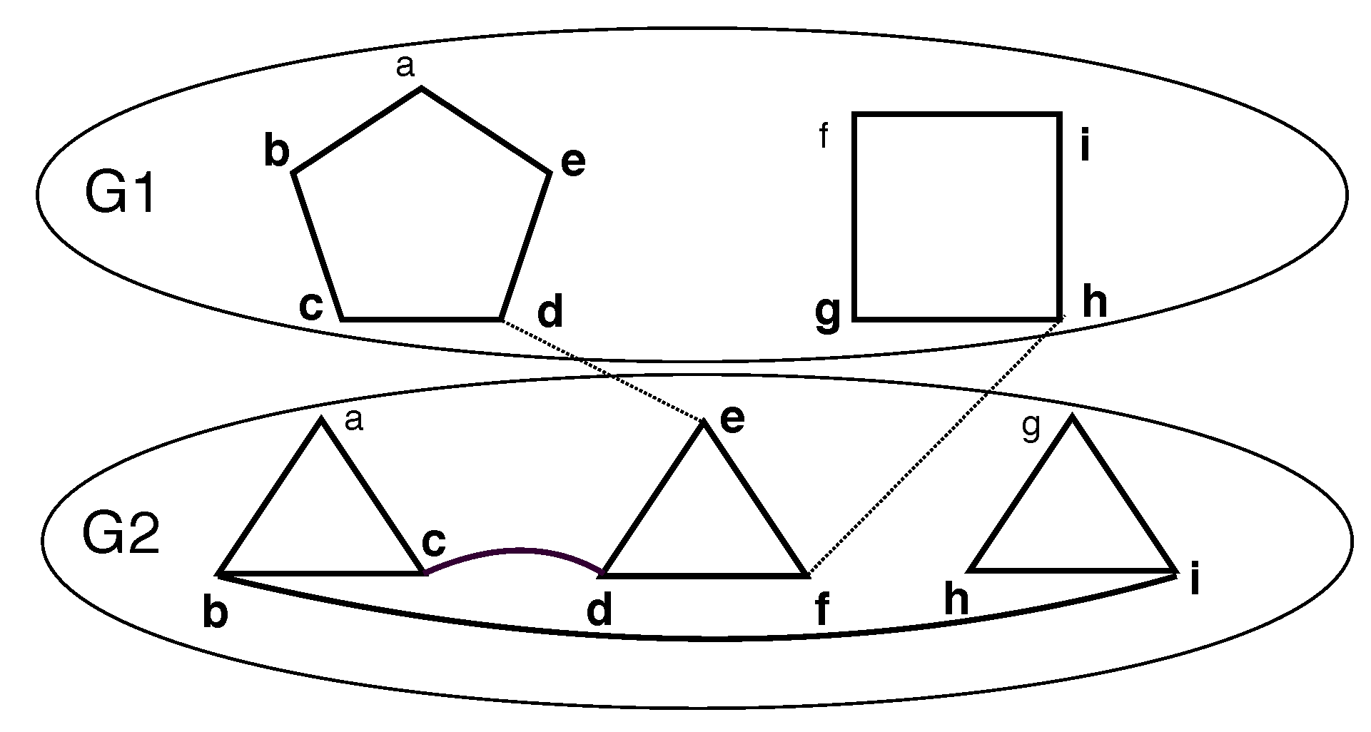
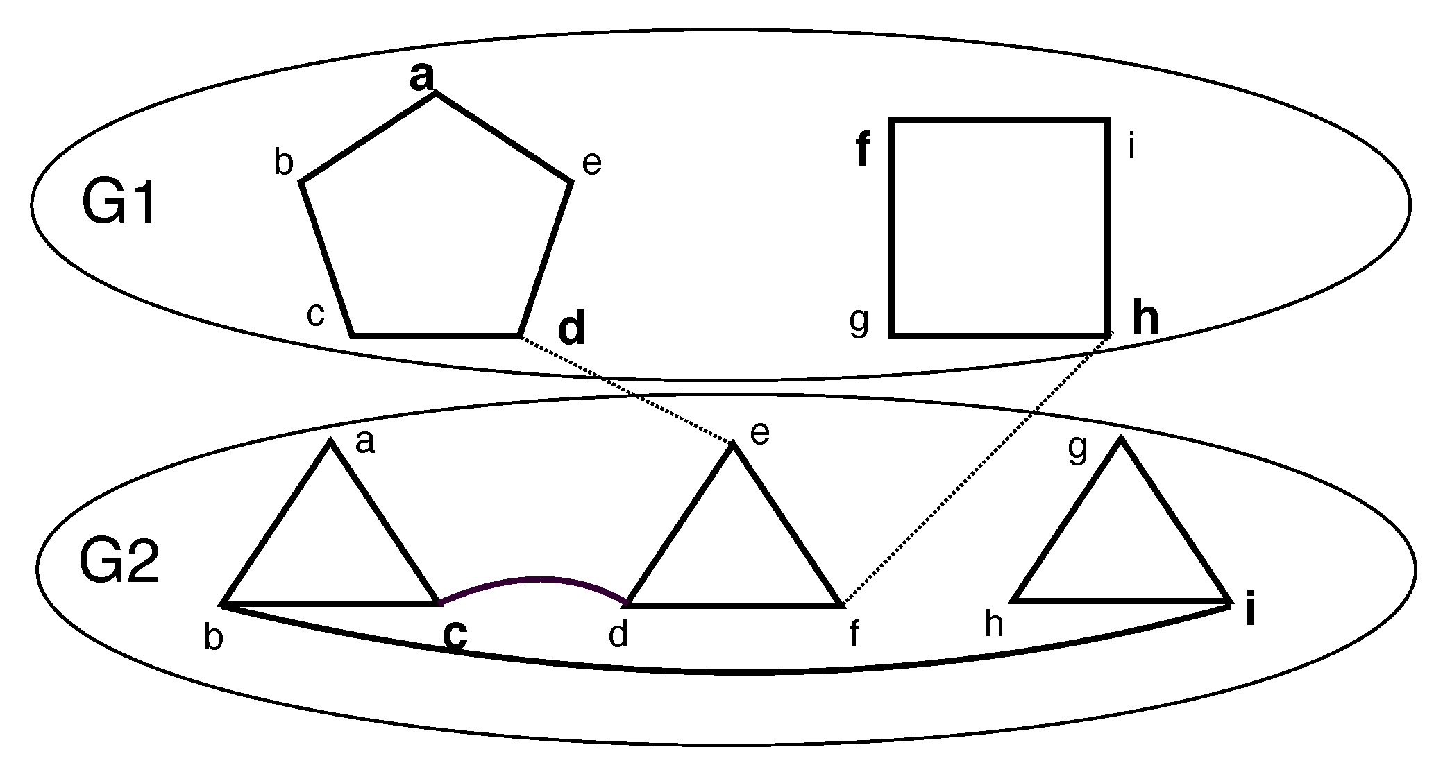
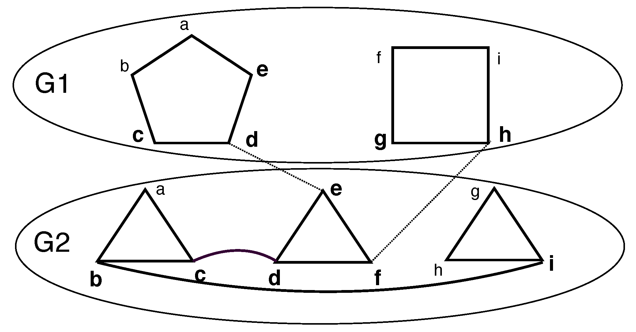
Consider a set of undirected graphs, , on the corresponding vertex sets () and the edge sets ( i.e., ). Consider a graph, G, that is formed from with special additional edges called inter-layer edges, denoted as , where and denotes the edges between and . We call such a graph a layered graph, denoted as , where the i-th layer is . Note that for any given i, , where can be and . Every vertex within a given layer gets a label from . Thus, . Note that is the vertex number, x, in layer i. However, in layer i, the vertex number, x, may not exist. Further, if , then it follows that vertex x is present in layer i and vertex y is present in layer .
We defined the following restrictions on a layered graph. Several of the these restrictions can be combined. Please see
Figure 1.
If , then a k-restricted layered graph, i.e., , is obtained. denotes an with q layers. denotes an with n vertices.
If , is an inter-layer edge , then a linear layered graph, i.e., , is obtained. denotes an that is k-restricted.
If is a connected component, then a single component layered graph, i.e., , is obtained.
If G is required to be a connected component, then a connected layered graph, i.e., , is obtained.
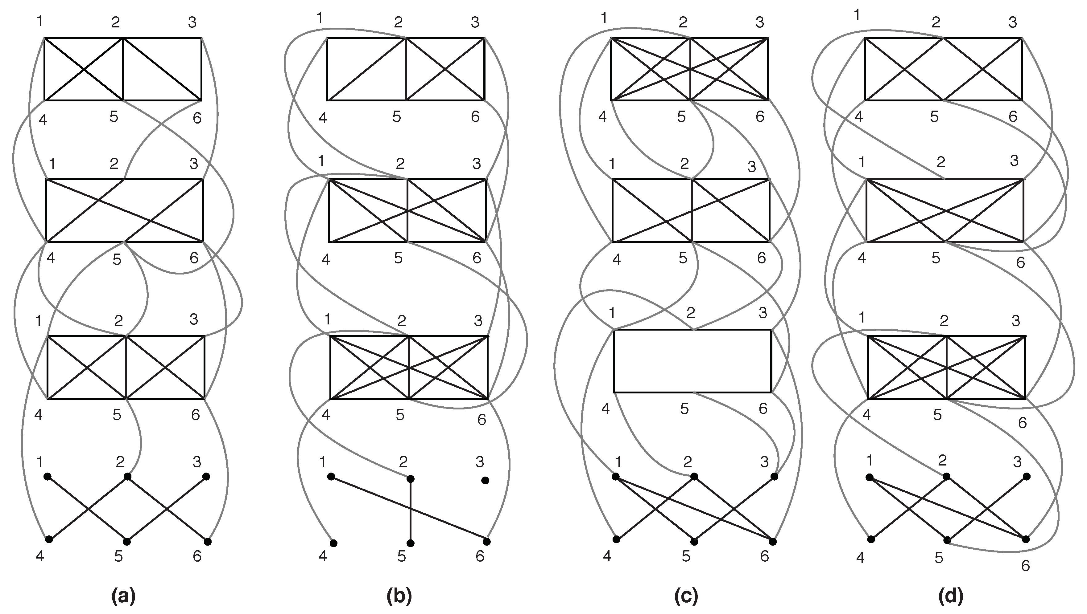
The problems of computing the adjacent swap distance between unsigned strings, adjacent swap distance between signed strings and short reversal distance were addressed in [
1]. If the alphabet is
,
is
k, the source string is
and the destination string is
and the length of
(and
) is
n, a
pairing diagram can be drawn for
and
, where all elements of
and
are treated as vertices, and perfect matching is performed on all
vertices, where each edge corresponds to (
,
) (here, both
,
denote the same symbol [
1]). The solutions to the above problems are based on
optimum pairing (in contrast to any perfect matching), where there is an edge from the
i-th occurrence of a symbol
x in
to the
i-th occurrence of
x in
; the corresponding pairing diagram is the
optimum pairing diagram. The solutions for adjacent swap distances are complete. However, the solution suggests that the short reversal distance is partial; it can solve very few sub-cases. Several distance problems on strings have been shown to be NP-complete [
30]. However, the complexity of short reversal distance problem is unknown. The short reversal distance was studied in [
2]. It was shown that the edges corresponding to two consecutive occurrences of a symbol
x in optimum pairing form a special edge-pair if they meet certain criteria. A conflict graph,
G, is constructed from an optimum pairing diagram where a vertex denotes a special edge-pair, and an edge exists between a pair of vertices that are in conflict. The computation of the short reversal distance is reduced to the computation of MIS on
G.
G consists of several subgraphs,
, each having, at most,
k vertices, where each vertex corresponds to a symbol in
. Each
is a subgraph of the
clique. The vertices,
, can have a conflict only if they correspond to the same symbol. Further, they share a common edge in the optimum pairing diagram. In this particular scenario, the layered graphs arise naturally. Further, such layered graphs are LLGs. In this framework, the computation of MIS on a LLG is a necessary component in the computation of the corresponding short reversal distance.
Considering a tribal society
S consisting of some villages on a bank of a river, a village consists of a few families where each family has its own
family-head. The family-heads of a given village know one another, and they also interact with specific family-heads of adjacent villages for trade (of produce) and partnership (collaboration in farming etc.). If one models this society as a social network, where a family-head is denoted by a vertex and an interaction (among family-heads) is denoted by an edge, then one obtains a layered graph. In this social network, identifying the smallest set of influencers is a natural pursuit (whose solution is given by computing MDS). These applications motivate the study of MIS, MDS and other graph theoretic problems on layered graphs. In general, graph theoretic problems, like subgraph isomorphism, and its variations have extensive applications in computational biology, e.g., references [
31,
32].
This article designs algorithms for where every vertex within a given layer gets a label from . The results are applicable for any restrictions of , like , , etc. Consider a layered graph, G, whose first a layers and last b layers do not have any edges. The graph is not a ; however, the MCV of G is the same as the MCV of the subgraph where the first a and the last b layers are removed. Further, if every layer has at least one intra-layer edge, then MCV can be computed only on . MCD is well defined only for because it must dominate all vertices.
The complete graph on k vertices, a clique on k vertices, is denoted by . Consider a graph, G, formed from several copies of , say , where, in addition to the edges that exist in each of , an edge is introduced between every pair, : and . We denote this particular graph, G, that has q layers with . The class of k-restricted layered graphs are in fact subgraphs of . Thus, we call a full . Likewise, a that is defined on q cliques, where for any , for all values of l, an edge is introduced between vertex l of layer i and vertex l of layer , is called a full. The number of layers in i.e., q is bound by .
A subgraph of G induced by vertices consists of all vertices () and all the edges restricted to them. We designed algorithms that compute the cardinalities of MVC, MIS and MDS of any subgraph of i.e., in polynomial time when and the cardinalities of MCV and MCD in polynomial time when , . Additionally, these algorithms report the corresponding numbers of MISs, MVCs, MDSs, MCVs and MCDs in .
3. Algorithm
Consider a layered graph with q layers, i.e., with layers . We designed a generic dynamic programming algorithm for all of the problems. However, certain restrictions exist corresponding to the problem at hand. The specific details pertaining to each problem are elucidated along with its solution. For example, MCD is meaningful only when the underlying graph is connected, i.e., the input graph is restricted to .
We denoted the vertices chosen in a particular layer with a k-bit variable that we called . The pth bit of the mask was set to one to include the pth vertex. Otherwise, the bit was set to zero and the vertex was excluded. Let be a candidate solution for a problem where denotes the set of nodes that are chosen from layer i. The candidate sub-solution for layer i is denoted . For layers , a combined candidate sub-solution is maintained, denoted . Likewise, and denote the sub-solutions (of layer i and first i layers respectively), where the vertices chosen from layer i are denoted by mask j. Only the cardinality of the best options is stored; such cardinality is called an optimum value. This is stored in the variable , and the corresponding number of solutions that yield the optimum value is stored in . In this article, an optimal solution is a solution that corresponds to the optimum value. We say that and are compatible if . That is, the union of and yields a for the first i layers. Note that compatibility is determined by and , and the vertices chosen by in the earlier layers are irrelevant. This is a key feature.
3.1. Input
The input consists of which is specified in terms of and , where is the 0–1 adjacency matrix for layer i, i.e., . is the 0–1 adjacency matrix for . Rows of correspond to vertices , and columns of are vertices . It must be noted that for a linear graph, can just be a k dimensional vector and the corresponding computation is less expensive where an edge between exists. The adjacency matrix , for layer i, is a matrix of dimensions , which means it requires space. Similarly, each also requires space. Therefore, the total space required for the input graph is , since each layer requires space, and there are layers.
The Boolean valued function compatible (please see Algorithm 1) determines whether the candidate sub-solutions (of the current layer and the subgraph induced by vertices of all previous layers) can be combined; here, the layer number, i, is implicit. For each mask, j, of a given layer, i, the function determines if j is a feasible option for layer i. The helper function, , returns the number of bits that are set in the binary representation of mask j.
All algorithms consist of the following sequence of computational tasks:
Repeat (i) and (ii) for all layers .
(i) Feasible: (if ), then go to step(ii).
(ii) Extension: If j and l are compatible, then store the cardinality of in and the count of in .
(iii) Summarize: At layer , execute (i) and (ii). Identify the optimum cardinality among and the corresponding count.
A particular problem has specific characteristics. In the sequel, where a problem is dealt with in detail, the corresponding validity/compatibility and other specifics are elucidated.
| Algorithm 1 Compatible Algorithm |
Input: , j, l, and I. //The function call: . l: Mask for layer i. Output: 0 (incompatible) or 1 (compatible). //j: Mask for layer . I denotes matrix for . // returns true if bit c is set in i, otherwise, it returns false. Case MIS: // Input: two valid MISs of two adjacent layers if then // : for any and : return 1; //if , return 0; otherwise, return 1; algorithm. else return 0; //∃ a pair of vertices across the layers joined with an edge. end if Case MVC: // Input: two VCs of two adjacent layers if then // : where : return 1; // then return 1; otherwise, return 0; algorithm. else return 0; end if Case MCV: // Input: two masks of two adjacent layers; need not be MCVs of their respective layers. if then // : where : return 1; // and for each component of l, : else // then return 1; otherwise, return 0; algorithm. return 0; end if Case MDS: // Input: two masks of two adjacent layers, if then // : return 1; // : if , then return 1; otherwise, return 0; else // : if , then return 1; otherwise, return 0; return 0; // or is not dominated. algorithm. end if // is the set of all vertices neighboring any vertex in V Case MCD: // Input: two masks of two adjacent layers, // For each component of l, : if then // : return 1; // : if then return 1; otherwise return 0; else // : if then return 1; otherwise return 0; return 0; // or is not dominated. algorithm. end if // is the set of all vertices neighboring any vertex in V
|
3.2. MIS
Consider the structure of an MIS on
. Say,
where
are the vertices in MIS from layer
j. Clearly,
must be an independent set. (please see
Figure 2). Let
be the subgraph of
induced by
, and let
be the subgraph of
induced by
. Consider the IS of
G. If
and
, then
and
are ISs. Let the set of edges crossing the cut,
, be
. It follows that
is an IS of
G with cardinality
when there is no edge crossing
C. Only the edges in
need to be considered. Thus, the cardinality of an MIS of
is equal to
.
: The mask j must denote an IS for .
: The union of two ISs must be an IS.
Extension: If .
Summarize: Let ; ; ; Return
3.3. MVC and MCV
Consider a vertex cover
of
where
denotes the set of vertices in
from layer
j. Clearly,
is a VC for layer
j (please see
Figure 3).
depends only on
and
. Consider two adjacent layers,
p and
.
must cover all inter-layer edges between layers
p and
. Specifically,
must cover all edges in the corresponding induced subgraph, including
. Similar constraints hold for MCV. Additionally, for MCV, the induced subgraph of
must be a connected component (please see
Figure 4). In the sequel, the time and space complexity analyses for these problems are presented.
Clearly, each layer must choose a mask that is a VC. In the case of MCV, when considering a mask, j, for the current layer, i, the following cases exist:
- (a)
The previous layer mask, l, corresponds to one component.
- (b)
l has more than one component, i.e., the set of vertices denoting l is partitioned into several connected components.
Case (a): For layer i, mask j is infeasible if either (I) vertices corresponding to j and l have no edges among them or (II) all edges in are not covered. Otherwise, j is feasible. If at least one edge exists across j and l:
- (i)
If j is a single connected component, then the result is also a single component (consisting of all chosen vertices).
- (ii)
If j has more than one connected component and all of them connect to l, then the result is also a single component.
- (iii)
If j has more than one connected component and only some of them connect to l, then the result consists of many components. All components from j connected to l become one component and the rest are separate components.
Case (b): Every component from the previous layer corresponding to mask l must connect to some component in the current layer. Otherwise, the pair j and l is infeasible for layer i. For feasible pairs the following possibilities exist:
- (i)
Every component in l has an edge with exactly one component in j. Here, the partition is determined by j.
- (ii)
A component, C, in l has edges with in j. Then, can be merged into one component as they are connected through C.
A particular partitioning of the current layer can occur due to various choices of l. For each partition corresponding to j, the sub-solution is stored with minimum cardinality. Thus, for each mask, j, there are, at most, (k-th Bell number) solutions stored. When mask x is chosen for the last layer, then the vertices of the mask must be connected to the components of the previous layer and yield a single component.
: Mask j must denote a VC for .
: The union of two VCs must be a VC for edges in and . i is the current layer. For MCV, all components of l must have edges with vertices in j. If , then must be one component.
Extension: If .
Summarize: Let ; ; ; Return
3.4. MDS and MCD
Let an MDS of
be
, such that,
, where
represents the vertices in this MDS from layer
j. Clearly,
may not be a dominating set of layer
j because the vertices of
can be dominated by any subset of
. In
Figure 5,
is dominated by
. It follows that
must dominate all vertices in
. Further,
must dominate
. A vertex that is not dominated is
undominated.
Consider mask j in layer i, where dominates layer . This particular subset of vertices can leave some vertices in layer i undominated. The number of such choices is ; each choice is denoted by a k-bit variable that we call a mask—here, a mask of exclusion. Further, when one processes layer , this information is critical. We show that the triples stored for each mask of a given layer suffice to compute MDS of . For a chosen mask, j, in layer i, it suffices to store triples of the form . Here, u is the mask of the vertices that are undominated in layer i, s is the cardinality of the vertices chosen so far and c is the number of choices corresponding to u for a particular j in layer i.
MCD has an additional requirement compared to MDS, i.e.,
must form a single component (please see
Figure 6). For possible combinations of component layouts of the current and previous layer masks, see MCV. For MCD, it suffices to store
triples of the form
, where
is the
k-th Bell number. This corresponds to
component layouts,
, for a mask,
j, and
masks
of the vertices that are
not dominated in layer
i and
triples
r of the form
for every unique pair of
. Here,
m is the mask of the current layer that produces the respective
pair, i.e., mask
j, while
s and
c are same as that for MDS, corresponding to mask
m and pair
. The particular mask in the previous layer that is the cause of a particular triple in the current layer needs not be carried forward. So, for MDS,
indicates an array of
triples. As for MCD, it indicates
triples where
triples are associated with each of the
unique pairs of
. Also, when
for MDS and
where
for MCD, the algorithm runs in polynomial time.
Consider the following analysis for MDS. Let mask j be chosen in layer i; it can potentially be combined with every mask ( masks) of the previous layer. Thus, potentially, () triples need be stored. Further, the total number of triples of the form is , because can potentially assume any ; s is and c can, in fact, be exponential in . Here, we make the following critical observations:
Let the chosen mask for layer i be j. When all the compatible vertex sets of the previous layer are considered, then let the resultant triples for the choice of j in layer i be set as S.
In S, for any two triples with the same mask, we need only to retain the triples with the smallest size. The other triples cannot lead to an optimal solution.
If two triples have the same mask and the minimum size, then they can be combined into one triple where the respective counts are added.
Thus, only triples suffice for a chosen mask for layer i which implies triples suffice . The information of only two layers is stored. Thus, the algorithm needs space. This is in addition to the space required by the input graph, which is . For , is the dominating term, so the space complexity is .
Thus, for a chosen mask for layer i, potentially triples of the previous layer must be processed. That is, for all masks of layer i, a total of triples must be processed.
Consider mask j in layer i and mask l in layer . Recall that there are triples stored corresponding to mask l in layer . All the vertices that are covered by the combination of j and l in layer , say A, and not covered in layer i, say B, can be computed in . This needs to be computed only once. Subsequently, for each of the triples stored corresponding to l in layer , we need only to check if the undominated vertices are a subset of B in time. Thus, is the dominating term in the time complexity, yielding for all masks in the previous layer. So, for all masks in the current layer, the time complexity is . Thus, the time complexity of the algorithm is .
Similar constraints hold for MCD. We carry forward the existing connected components, and eventually, when the final layer is processed, all the components must be connected. The MCD algorithm is explained in detail in Theorem 4 along with time and space complexity analyses. The current layer in the following functions is i.
: Any j is valid.
: Tthe union must dominate all vertices of . For MCD, all components of l must have edges with vertices in j. If , then must be one component and it must dominate also.
Extension: Performed as per the observations listed above.
Summarize: Let ; ; if then ; return .
3.5. Compatible Algorithm
Given candidate sub-solutions for consecutive layers one must determine if their union is a feasible sub-solution. The following algorithm determines the same for the problems addressed in this article.
3.6. Generic Optimum Algorithm
The algorithms (please see Algorithm 2) for the MIS, MVC and MDS problems on
are similar, while those for MCV and MCD must additionally ensure connectedness criterion. We give a generic dynamic programming based algorithm for both sets of problems. Some specific instances are shown in
Appendix A.
Initialization: ; ; The optimum value (of IS, VC, MCD, etc.) up to layer i, where the chosen vertices of layer i are given by the binary value of j. The number of ways that the j-th mask in layer i yields the corresponding optimum value.
| Algorithm 2 Generic Optimum Algorithm |
Input: Output: The cardinality and corresponding count for the respective problem. for () do if then //for layer 1 // For all valid masks, set their count end if end for for () do //For layers 2 through maximum for do //For all masks of the current layer Compose larger sub-solutions by considering all compatible masks of the previous layer and any accompanying information. end for//Masks of previous layer end for//For all layers, The current layer being processed is the final layer. for () do Identify , the cardinality of an optimal solution. end for for () do Compute , the count of the optimal solutions. end for
|
4. Correctness and Complexity
The Algorithm Generic Optimum when adapted to a specific problem, say MVC, is referred to as Algorithm MVC. The correctness is shown for MIS, MVC and MCD problems. The time complexities for MIS, MVC, and MDS are respectively , and , where . When these time complexities yield , and respectively. The space complexities are , and respectively. When these space complexities yield , and respectively. For MCV and MCD problems, the time complexity is for any , where the number of vertices in a layer is for . The space complexity is for MCD and MCV. The time and space complexities of MVC and MCD are analyzed. The proofs of correctness for the remaining problems are similar. The time complexity for MDS was presented earlier.
Theorem 1. The MIS Algorithm correctly computes the MIS on .
Proof. Let be a graph and let V be partitioned into . Further, let be the ISs of the graphs induced by , respectively, and let . If we consider the cut, , on I, where is the set of edges crossing the cut, then it follows that I is an IS of G if . Further, the cardinality of an MIS of G is . It is possible that either or .
Let G be . Let be the subgraph of induced by , and let be the subgraph of , induced by . Consider the IS of G. Let and be the independent sets of and , respectively. Let the set of edges crossing the cut, , be . It follows that is an IS of G with cardinality when there is no edge crossing C. Only the edges in need to be considered. Thus, the cardinality of an MIS of is equal to . When the last layer is processed, the cardinalities of the ISs of subgraphs induced by both V and are known. Further, these ISs have maximum cardinalities with respect to the vertices chosen in layers and q, respectively. The theorem follows. Likewise, gives the number of ways that an independent set of maximum cardinality can be formed when the vertices chosen in layer i are given by j. Thus, the corresponding to the maximum value of yields the total number of MISs. ☐
Theorem 2. The MVC Algorithm correctly computes the MVC on .
Proof. Consider the structure of MVC on . Let be the subgraph of induced by , and let be the subgraph of induced by . Consider a VC of G. Let and be the vertex covers of and , respectively. Let the set of edges crossing the cut, , be . It follows that the cardinality of a VC of G is when every edge crossing C is covered by either or . Note that the only edges from can go across the cut. Thus, the cardinality of the MVC of is equal to for any such cut. When the last layer is processed, this property is ensured. The theorem follows. Similarly, gives the number of ways that a vertex cover of minimum cardinality can be formed when the vertices chosen in the layer i are given by j. Thus, corresponding to the minimum value of yields the total number of MVCs. ☐
Theorem 3. The MVC Algorithm on runs in polynomial time in n when . The space required is .
Proof. We presume that , the 0–1 adjacency matrix for the subgraph induced by where the edges are restricted to is given. Likewise, we assume that the 0–1 adjacency matrix, , for each of is given. Recall that was formed from . For a linear graph, is just a -dimensional vector where, if bit j is set, then there is an edge between and .
The initialization step requires time.
Given a mask for layer i, it can be determined whether VC is valid in time with . That is, for any two that are set, the mask should have either a bit a or a bit b set.
Given and two masks, and , for layers i and , respectively, it can be directly determined whether the union of the two masks is a VC of the subgraph induced by , of , in time.
In order to determine the MVC up to layer i, whose mask is j, j must be checked for compatibility with all masks of the previous layer. Thus, time is required. For all masks of the current layer, , time is required. For all layers, the time required is maximized when each layer has k vertices yielding = time.
The time complexity is clearly exponential in k; however, if , the time complexity is . The time complexity remains polynomial when ; specifically, when . The additional space required is because for two layers, masks and count variables are stored, each of size k. The space required is to store the graph and an additional space of that is needed by the algorithm. When , the space complexity is . ☐
Lemma 1. Let , where . If , then for any .
Proof. Let , . Let .
Thus,
. Taking log on both sides we obtain:
Disregarding smaller order terms we obtain the expression: = . Note that for any . Thus, for any . Given that one can always choose such that . Thus, the expression is for any .
Thus, . ☐
Lemma 2. is quasi-polynomial and .
Proof. From Stirling’s Approximation, we have
Thus, for some constants and ,
Thus, is quasi-polynomial. ☐
Lemma 3. If , for any then, the MIS Algorithm, MVC Algorithm and MDS Algorithm run in quasi-polynomial time.
Proof. The time complexities of all these algorithms can be written as , where , and . Thus, when for , the complexities for all the algorithms will be quasi-polynomial. ☐
Theorem 4. The MCD Algorithm correctly computes the cardinality of a connected minimum dominating set for with a time complexity of for any when and . The space complexity of the algorithm is .
Proof. First, we show that the algorithm correctly computes the cardinality of a connected minimum dominating set. Consider the structure of CDS on a connected graph, G. Let V be arbitrarily partitioned into , where both and . Let be the subgraph of G induced by , and let be the subgraph of G induced by . Let and be DSs of and . Let C be the cut and let be the edges that cross this cut. Clearly, is DS for G. Further, M is a CDS for G if , and M forms a connected component in G. For a given partition of V, M is a MCD if it minimizes , where M forms a connected component in G.
Let G be a ; in particular, let G be a . Let and . Let be the subgraph of G induced by , and let be the subgraph of G induced by . Let and be DSs of and , respectively. Let C be the cut , and let be the edges that cross this cut. Note that . When the algorithm processes layer q, it chooses , such that is minimized where M forms a connected component in G. Thus, the theorem follows. Similarly, gives the number of ways a CDS of minimum cardinality can be formed when the vertices chosen in layer i are given by j. Thus, corresponding to the minimum value of yields the total number of MDSs.
The time complexity of the algorithm is analyzed below. We presumed that similar prerequisites as in Theorem 3 were provided. The steps are presented below.
A global structure, , consisting of and , corresponding to the previous and current layers, is maintained for the whole algorithm. The final solution for the problem can be determined just by using information from and . This structure is maintained for the whole algorithm and not for every layer.
and consist of a maximum of triples of the form . This corresponds to a maximum of component layouts (), masks, undominated vertices of the current layer and a maximum of triples, r, of the form , for every unique pair . Here, m is the mask of the current layer that produced the respective (component layout, undominated vertices) pair; s is the minimum cardinality of the sub-solution corresponding to mask m and pair ; and c is the count of s corresponding to mask m and pair .
Throughout the algorithm, and are maintained by clearing when the current layer is processed and the information of is used as for the next layer.
is initialized with the triple , corresponding to masks of the first layer. The initialization takes .
A candidate sub-solution for layers induces connected components in layer i that are defined in terms of vertices of layer i. We call this the component layout.
The number of component layouts is upper bounded by , the number of ways of partitioning k vertices of a layer. Here, , , . . From Lemma 1, we know that =, for any .
A mask j of the current layer can be combined with a component layout for mask l of the previous layer to form a new component layout for the current layer. With the same mask, l, j can form a new mask corresponding to the undominated vertices of the current layer.
Every such unique pair of (, ), where is component layout and is mask of undominated vertices, is maintained, and a list of triples r, consisting of triples of the form , is associated with it. Here, m is the current layer mask, s is the minimum cardinality of the sub-solution corresponding to m, and c is the count of s. The number of such tuples, , is upper bounded by , where is the possible number of unique pairs of , and is the possible number of triples that can exist for each pair.
Starting from the i-th layer, , every masks of the current layer and the triple values from the previous layer are used to generate the triples for the current layer.
For a unique pair in the previous layer, if mask j dominates the undominated vertices of mask , and forms a connected component with the layout, , then we consider that a sub-solution using mask j is feasible. Here, a mask, j, and a component layout, , are considered to form a connected component if every component in has at least one edge with a node in mask j. Each such check takes time. So, the total time to determine if a sub-solution with mask j is feasible is .
If a mask, j, can feasibly give a sub-solution, then it is combined with the component layout, , of the previous layer to form a new component layout for the current layer corresponding to mask j. This is performed using a DFS which takes for the given input matrix.
Mask j is then combined with mask l of the previous layer, corresponding to the pair that is under consideration, to form a mask for the current layer vertices that are not dominated by j or l. This takes time.
Using the mask, j, of the current layer and minimum cardinality, s, for the pair of the previous layer, the new cardinality for the sub-solution is computed.
The count of the new cardinality will be same as that of c of the pair for the previous layer.
This new pair of the component layout and undominated mask computed for mask j of the current layer are checked with the existing pairs of the current layer to determine if it is unique or not. We maintain the structure of the triples such that an entry can be accessed in time, indexed by the pair and the corresponding mask m for the previous and the current layer.
If it is unique, the triple value, consisting of the newly computed pair and its corresponding triple, consisting of the mask j, respective cardinality and the count, are added as a new triple for the current layer.
Consider that the current mask j produces the new pair with values and . If the new pair is not unique, then there are three cases. Consider the existing entry of the pair and the corresponding j to have values and .
- (a)
If , then ;
- (b)
If , then ;
- (c)
If , then no update is required.
The above procedure is performed until the last layer, where the final solution is computed from the current layer information corresponding to the last layer. Of all the pairs for the current layer, a solution is considered to be feasible if the mask for the undominated vertices for any of the component layouts is 0, as this would mean all the vertices are dominated. The cardinality of MCD is the minimum value among all the feasible solutions. The count is then computed by considering each feasible entry with the minimum cardinality computed above and adding its corresponding count.
Thus, the solution and the corresponding count of optimal solutions for MCD problem are computed.
For the whole algorithm, we maintained a global structure, as mentioned above. It consisted of a maximum of entries corresponding to unique pairs of and another triples for each such pair. We maintainewa this information for only the previous and the current layers. So, the space used by the data structure is . This can be shown to be equal to , for any , based on the proof for Lemma 1. This space requirement is in addition to the space required by the input graph which is . For , is the dominating term compared to . So, the space complexity is . The following is the proof for time complexity of the algorithm.
First, an expression for the runtime of the algorithm is derived. The initialization using the first layer takes
time. For each layer after the first, the
masks of the current layer are combined with the
pairs of the previous layer. For each pair, a current layer mask is combined with a maximum of
masks of the previous layer that generated this pair. Checking the feasibility of a mask of the current layer takes
. Computing the new component layout and the new undominated mask takes
each. The undominated mask is calculated for
masks of the previous layer for each mask of the current layer. Accessing and updating an entry takes
time, as mentioned above. This is done for
layers. So, the time complexity expression can be written as
If , the time complexity becomes . If we assume the worst case number of nodes in each layer, i.e., , then the corresponding time complexity is . as shown below.
Let
Let
The running time of the algorithm is given by
Consider
Let and
We know that the logarithmic functions grow slower than the polynomial functions.
Now, we claim that for some , a positive real number c and , where is some positive intege.
Taking the log of both sides, we get
Since
,
Hence, we have proved our claim.
By arbitrarily taking small values for
,
and
,
can be any value, such that
.
Hence, the theorem is proved. ☐
Theorem 5. The MCV Algorithm correctly computes a connected VC of minimum cardinality for with a time complexity of for any when and . The space complexity is .
Proof. The MCV Algorithm is similar to the MCD Algorithm. A mask, j, of layer i must be a valid VC for layer i. The check takes an additional , though the total time complexity can be proved to be same as that of MCD. So, the proofs of correctness and time complexity follow from the proofs for the same of the MCD Algorithm. Hence, the time complexity is for any when the number of vertices in each layer is k, where and . Similarly, the space complexity can be shown to be . ☐
Lemma 2 proves that
is quasi-polynomial. Thus, if
then MCV and MCD are computed in quasi-polynomial time. Proving this is quite straightforward. By substituting
for
into Equation (
1) in Theorem 4, we get a product of a quasi-polynomial factor and a polynomial factor. Thus, the time complexity is quasi-polynomial.
Minor Enhancements
The current layer requires information only from the previous layer. So, only the variables of the current layer, i, and the previous layer, , are maintained. In the pseudocode shown for all algorithms, for simplicity, the variables of the current layer are stored at index 1 and the variables of the previous layer are stored at index 0 of the data structure . When the current layer, i, is completely processed, the variables from index 1 overwrite the corresponding variables in index 0. This can be avoided by alternating the index of current layer between indices 0 and 1, thereby reducing the execution time by a factor of .
The optimum cardinalities for each of the problems are generated using minimal additional space. For example, the MVC Algorithm employs only space in addition to the space required by the graph. If, for each mask in each layer, we store the best compatible mask from the previous layer, then we can generate a solution. There are layers, each having k-bit masks. This requires space instead of space. However, if we want to generate all solutions, then for each mask of a given layer, we need to store all compatible masks of its previous layer that yield the optimum value requiring space.


