Article

Optimal Control Algorithms and Their Analysis for Short-Term Scheduling in Manufacturing Systems

1
Saint Petersburg Institute for Informatics and Automation of the RAS (SPIIRAS), V.O. 14 line, 39, 199178 St. Petersburg, Russia
2
Department of Automation, Production and Computer Sciences, IMT Atlantique, LS2N—CNRS UMR 6004, La Chantrerie, 4 rue Alfred Kastler, 44300 Nantes, France
3
Department of Business Administration, Berlin School of Economics and Law, 10825 Berlin, Germany
*
Author to whom correspondence should be addressed.
Algorithms 2018, 11(5), 57; https://doi.org/10.3390/a11050057
Submission received: 18 February 2018 / Revised: 15 April 2018 / Accepted: 16 April 2018 / Published: 3 May 2018
(This article belongs to the Special Issue Algorithms for Scheduling Problems)

Abstract

:
Current literature presents optimal control computational algorithms with regard to state, control, and conjunctive variable spaces. This paper first analyses the advantages and limitations of different optimal control computational methods and algorithms which can be used for short-term scheduling. Second, it develops an optimal control computational algorithm that allows for the solution of short-term scheduling in an optimal manner. Moreover, qualitative and quantitative analysis of the manufacturing system scheduling problem is presented. Results highlight computer experiments with a scheduling software prototype as well as potential future research avenues.

1. Introduction

Short-term scheduling in manufacturing systems (MS) considers jobs that contain operation chains with equal (i.e., flow shop) or different (i.e., job shop) machine sequences and different processing times. Operations which need to be scheduled for machines with different processing power are subject to various criteria including makespan, lead time, and due dates ([1,2,3,4]).
Over the last several decades, various studies have investigated scheduling problems from different perspectives. A rich variety of methods and applications can be observed in the development of rigorous theoretical models and efficient solution techniques. [5,6,7,8,9,10,11,12] and [13] have demonstrated that specific large-scale scheduling problems with complex hybrid logical and terminal constraints, process execution non-stationary (i.e., interruptions in machine availability), complex interrelations between process dynamics, capacity evolution and setups (i.e., intensity-dependent processing times for machine work) require further investigation in terms of a broad range of methodical approaches. One of these is optimal control.
Optimal control approaches differ from mathematical programming methods and represent schedules as trajectories. The various applications of optimal control to scheduling problems are encountered in production systems with single machines [14], job sequencing in two-stage production systems [15], and multi-stage machine structures with alternatives in job assignments and intensity-dependent processing rates. Specifically, such multi-stage machine structures include flexible MSs ([16,17,18]), supply chain multi-stage networks ([19,20]), and Industry 4.0 systems that allow data interchange between the product and stations, flexible stations dedicated to various technological operations, and real-time capacity utilization control [13].
A diversity of knowledge and findings in optimal control applications exists which pertains to scheduling. However, these approaches typically pertain to trajectories which are assumed to be optimal but are subject to some specific constraint system and process model forms such as finite dimensionality, convexity, etc. In general, optimal control algorithms only provide the necessary conditions for optimal solution existence. The maximum principle provides both optimality and necessary conditions only for some specific cases, i.e., linear control systems. As such, further investigations are required in each concrete application case.
This paper seeks to bring the discussion forward by carefully elaborating on the optimality issues described above and providing some ideas and implementation guidance on how to confront these challenges. The purpose of the present study is to contribute to existing works by providing some closed forms of algorithmic optimality proven in the rich optimal control axiomatic.
The rest of this paper is organized as follows. In Section 2, we propose general elements of the multiple-model description of industrial production scheduling and its dynamic interpretation. In Section 3, optimal control computational algorithms and their analyses are proposed. Section 4 presents a combined method and algorithm for short-term scheduling in MS. In Section 5, qualitative and quantitative analysis of the MS scheduling problem is suggested. The paper concludes in Section 6 by summarizing the results of this study.

2. Optimal Control Applications to Scheduling in Manufacturing Systems

Optimal control problems belong to the class of extremum optimization theory, i.e., the analysis of the minimization or maximization of some functions ([21,22,23,24,25,26,27,28]. This theory evolved on the basis of calculus variation principles developed by Fermat, Lagrange, Bernulli, Newton, Hamilton, and Jacobi. In the 20th century, two computational fundamentals of optimal control theory, maximum principle [21] and dynamic programming method [29], were developed. These methods extend the classical calculus variation theory that is based on control variations of a continuous trajectory and the observation of the performance impact of these variations at the trajectory’s terminus. Since control systems in the middle of the 20th century were increasingly characterized by continuous functions (such as 0–1 switch automats), the development of both the maximum principle and dynamic programming was necessary in order to solve the problem with complex constraints on control variables.
Manufacturing managers are always interested in non-deterministic approaches to scheduling, particularly where scheduling is interconnected with the control function [30]. Studies by [31] and [11] demonstrated a wide range of advantages regarding the application of control theoretic models in combination with other techniques for production and logistics. Among others, they include a non-stationary process view and accuracy of continuous time. In addition, a wide range of analysis tools from control theory regarding stability, controllability, adaptability, etc. may be used if a schedule is described in terms of control. However, the calculation of the optimal program control (OPC) with the direct methods of the continuous maximum principle has not been proved efficient [32]. Accordingly, the application of OPC to scheduling is important for two reasons. First, a conceptual problem consists of the continuous values of the control variables. Second, a computational problem with a direct method of the maximum principle exists. These shortcomings set limitations on the application of OPC to purely combinatorial problems.
To date, various dynamic models, methods and algorithms have been proposed to solve planning and scheduling problems in different application areas ([13,19,33,34,35,36,37,38]). In these papers, transformation procedures from classical scheduling models to their dynamic analogue have been developed. For example, the following models of OPC were proposed:
  • M g 
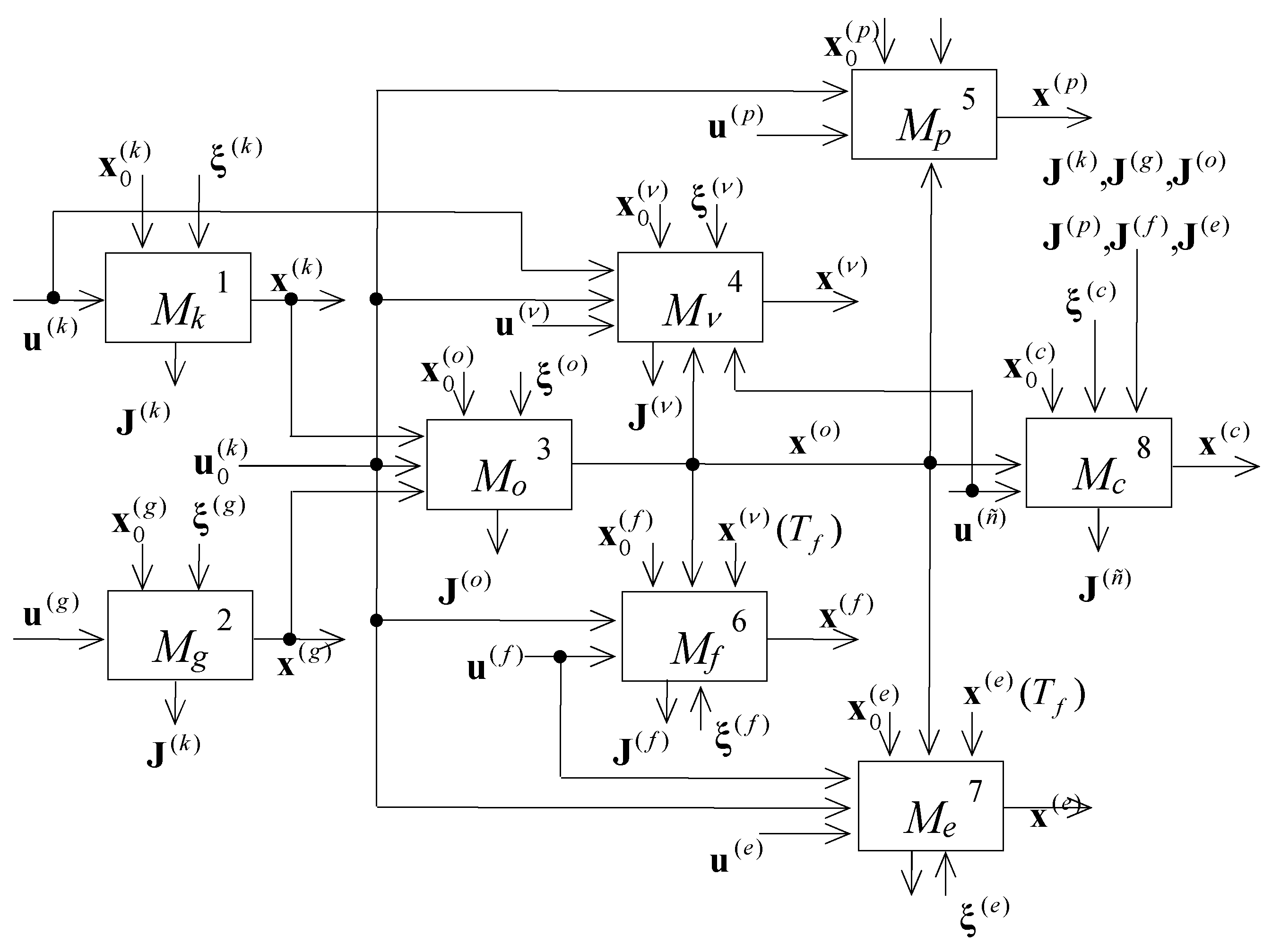
—dynamic model of MS elements and subsystems motion control;
  • M k —dynamic model of MS channel control;
  • M o —dynamic model of MS operations control;
  • M f —dynamic model of MS flow control;
  • M p —dynamic model of MS resource control;
  • M e —dynamic model of MS operation parameters control;
  • M c —dynamic model of MS structure dynamic control;
  • M ν —dynamic model of MS auxiliary operation control.
The detailed mathematical formulation of these models was presented by [36,37] as well as [38]. We provide the generalized dynamic model of MS control processes ( M model) below:
M = { u ( t ) | x ˙ = f ( x , u , t ) ; h 0 ( x ( T 0 ) ) O , h 1 ( x ( T f ) ) O , q ( 1 ) ( x , u ) = O , q ( 2 ) ( x , u ) < O } ,
J ϑ = J ϑ ( x ( t ) , u ( t ) , t ) = φ ϑ ( x ( t f ) ) + T 0 T f f ϑ ( x ( τ ) , u ( τ ) , τ ) d τ , ϑ { g , k , o , f , p , e , c , ν } ,
where ϑ { g , k , o , f , p , e , c , ν } —lower index which correspond to the motion control model, channel control model; operations control model; flow control; M p —resource control; operation parameters control; structure dynamic control model; auxiliary operation control model; x = x ( g ) T , x ( k ) T , x ( o ) T , x ( p ) T , x ( f ) T , x ( e ) T , x ( c ) T , x ( v ) T T is a vector of the MS generalized state, u = u ( g ) T , u ( k ) T , u ( o ) T , u ( p ) T , u ( f ) T , u ( e ) T , u ( c ) T , u ( v ) T T is a vector of generalized control, h 0 , h 1 are known vector functions that are used for the state x end conditions at the time points t = T 0 and t = T f , and the vector functions q ( 1 ) , q ( 2 ) define the main spatio–temporal, technical, and technological conditions for MS execution; J ϑ are indicators characterizing the different aspects of MS schedule quality.
Overall, the constructed model M (1) is a deterministic, non-linear, non-stationary, finite-dimensional differential system with a reconfigurable structure. Figure 1 shows the interconnection of models M g , M k , M o , M p , M f , M e , M c , and M ν embedded in the generalized model.
In Figure 1 the additional vector function ξ = ξ ( g ) T , ξ ( k ) T , ξ ( o ) T , ξ ( p ) T , ξ ( f ) T , ξ ( e ) T , ξ ( c ) T , ξ ( v ) T T of perturbation influences is introduced.
The solutions obtained in the presented multi-model complex are coordinated by the control inputs vector u ( o ) ( t ) of the model Mo. This vector determines the sequence of interaction operations and fixes the MS resource allocation. The applied procedure of solution adjustment refers to resource coordination.
The model complex M evolves and generalizes the dynamic models of scheduling theory. The predominant distinctive feature of the complex is that non-linear technological constraints are actualized in the convex domain of allowable control inputs rather than in differential equations [36,37].
In this case, the MS job shop scheduling problem can be formulated as the following problem of OPC: it is necessary to find an allowable control u ( t ) , t ( T 0 , T f ] that ensures for the model (1) meeting of vector constraint functions q ( 1 ) ( x , u ) = 0 , q ( 2 ) ( x , u ) 0 and guides the dynamic system (i.e., MS job shop schedule) x ˙ ( t ) = f ( t , x ( t ) , u ( t ) ) , from the initial state to the specified final state. If there are several allowable controls (schedules), then the best one (optimal) should be selected to maximize (minimize) J ϑ . The formulated model is a linear, non-stationary, finite-dimensional, controlled differential system with the convex area of admissible control. Note that the boundary problem is a standard OPC problem ([21,36,37]). This model is linear in the state and control variables, and the objective is linear. The transfer of non-linearity to the constraint ensures convexity and allows use of interval constraints.
In this case, the adjoint system can be written as follows:
ψ ˙ l = H x l + α = 1 I 1 λ α ( t ) q α ( 1 ) ( x ( t ) , u ( t ) ) x l + β = 1 I 2 ρ β ( t ) q β ( 2 ) ( x ( t ) , u ( t ) ) x l
The coefficients λα(t), ρβ(t) can be determined through the following expressions:
ρ β ( t ) q β ( 2 ) ( x ( t ) , u ( t ) ) 0 , β { 1 , , I 2 }
grad u H ( x ( t ) , u ( t ) , ψ ( t ) ) = α = 1 I 1 λ α ( t ) grad u q α ( 1 ) ( x ( t ) , u ( t ) ) + β = 1 I 2 ρ β ( t ) grad u q β ( 2 ) ( x ( t ) , u ( t ) )
Here, xl are elements of a general state vector, ψl are elements of an adjoint vector. Additional transversality conditions for the two ends of the state trajectory should be added for a general case:
ψ l ( T 0 ) = J o b x l | x l ( T 0 ) = x l 0 , ψ l ( T f ) = J o b x l | x l ( T f ) = x l f
Let us consider the algorithmic realization of the maximum principle. In accordance with this principle, two systems of differential equations should be solved: the main system (1) and the adjoint system (2). This will provide the optimal program control vector u * ( t )  (the indices «pl» are omitted) and the state trajectory x * ( t ) . The vector u * ( t ) at time t = T0 under the conditions h0 (x(T0)) ≤ 0 and for the given value of ψ ( T 0 ) should return the maximum to the Hamilton’s function:
H ( x ( t ) , u ( t ) , ψ ( t ) ) = Ψ T f ( x , u , t )
Here we assume that general functional of MS schedule quality is transformed to Mayer’s form [21].
The received control is used in the right members of (1), (2), and the first integration step for the main and for the adjoint system is made: t1 = T0 + δ ˜ ( δ ˜ is a step of integration). The process of integration is continued until the end conditions h 1 ( x ( T f ) ) O are satisfied and the convergence accuracy for the functional and for the alternatives is adequate. This terminates the construction of the optimal program control u * ( t ) and of the corresponding state trajectory x * ( t ) .
However, the only question that is not addressed within the described procedure is how to determine ψ ( T 0 ) for a given state vector x ( T 0 ) .
The value of ψ ( T 0 ) depends on the end conditions of the MS schedule problem. Therefore, the maximum principle allows the transformation of a problem of non-classical calculus of variations to a boundary problem. In other words, the problem of MS OPC (in other words, the MS schedule) construction is reduced to the following problem of transcendental equations solving:
Φ = Φ ( ψ ( T 0 ) ) = 0
At this stage, we consider the most complicated form of the MS OPC construction with MS initial state at time t = T0. The end point of the trajectory and the time interval are fixed:
x ( T f ) = a
where a = | | a 1 , a 2 , , a n ˜ | | T is a given vector; n ˜ is the dimensionality of the general MS state vector. Hence, the problem of optimal MS OPC construction is reduced to a search for the vector ψ ( T 0 ) , such that:
Φ = Φ ( ψ ( T 0 ) ) = x ( T f ) a
The problem of solving Equations (9) is equivalent to a minimization of the function:
Δ u ( ψ ( T 0 ) ) = 1 2 ( a x ( T f ) ) T ( a x ( T f ) )
The main feature of the problems (9), (10) is that the interdependency of ψ ( T 0 ) and ρ ( T f ) = ( a x ( T f ) ) is defined indirectly via the system of differential Equation (1). This feature leads to the use of iterative methods.

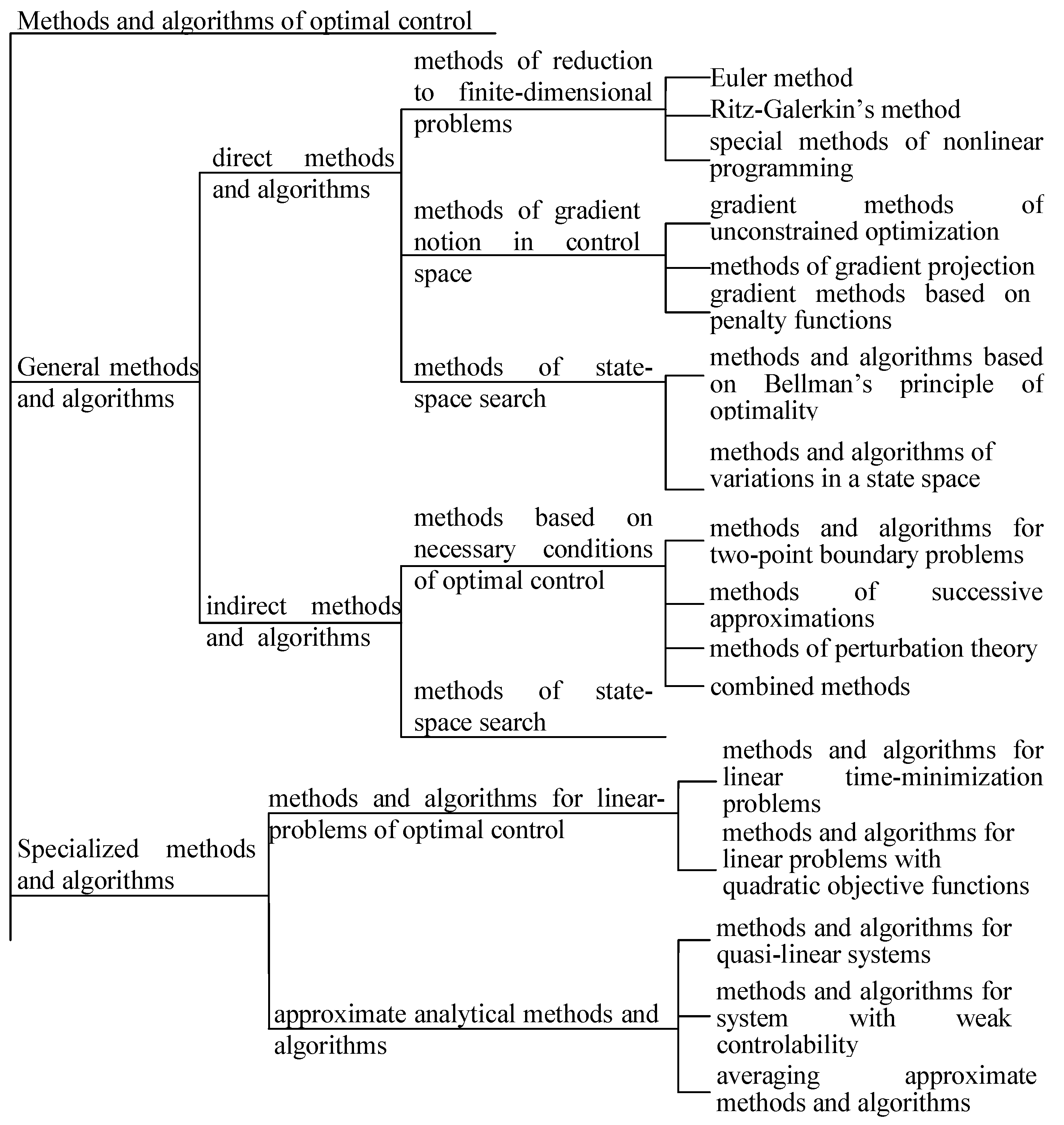
3. Classification and Analyses of Optimal Control Computational Algorithms for Short-Term Scheduling in MSs

Real-world optimal control problems are characterized by high dimensionality, complex control constraints, and essential non-linearity. Prior to introducing particular algorithms and methods of optimal control computation, let us consider their general classification (Figure 2).
Two main groups are distinguished: the group of general optimal control algorithms and methods and the group of specialized algorithms. The first group includes direct and indirect methods and algorithms. The direct methods imply search processes in spaces of variables. The first and most widely used methods of this group are the methods of reduction to finite-dimensional choice problems. Another subgroup includes direct gradient methods of search in functional spaces of control. To implement complex constraints for control and state variables, the methods of penalty functions and of gradient projection were developed. The third subgroup represents methods based on Bellman’s optimality principle and methods of variation in state spaces. The methods of this subgroup help to consider various state constraints.
Unlike the methods of the first group, the indirect methods and algorithms are aimed at the acquisition of controls that obey the necessary or/and sufficient optimality conditions. Firstly, the methods and algorithms for two-point boundary problems can be referenced. Particular methods are used here: Newton’s method (and its modifications), Krylov and Chernousko’s methods of successive approximations, and the methods of perturbation theory.
Methods based on sufficient conditions of optimality are preferable for irregular problems such as optimal zero-overshoot response choice. The third group includes specialized methods and algorithms for linear optimal control problems and approximate analytical methods and algorithms. The latter methods imply that the nonlinear components of models are not essential.
Let us limit a detailed analysis of computational procedures to two-point boundary problems with fixed ends of the state trajectory x ( t ) and a fixed time interval ( T 0 , T f ] . For this system class, the following methods can be considered ([23,24,33]): Newton’s method and its modifications, methods of penalty functionals, gradient methods, and the Krylov–Chernousko method.
Let us consider the possible implementation of the above-mentioned methods to the stated problem.
Newton’s method and its modifications. For the first iteration of the method, an initial approximation ψ ( T 0 ) = ψ ( 0 ) ( T 0 ) is set. Then, the successive approximations are received from the formula:
ψ ( r ) ( T 0 ) = ψ ( r 1 ) ( T 0 ) [ ρ ( r 1 ) ( T f ) ψ ( r 1 ) ( T 0 ) ] ρ ( r 1 ) ( T f )
where ρ ( r ) ( T f ) = a x ( r 1 ) ( T f ) , r = 1, 2, ….
The operation of partial derivation, being performed at all iterations, is rather complicated. Here the derivative matrix:
Π ˜ = ( ρ ( r 1 ) ( T f ) ψ ( r 1 ) ( T 0 ) )
should be evaluated.
This matrix can be received either via finite-difference formulas or via a variational integration of the system. Modification of the method can also be used. The following method is the simplest. The formula (11) is substituted for:
ψ ( r ) ( T 0 ) = ψ ( r 1 ) ( T 0 ) γ ( r ) Π ˜ 1 ρ ( r 1 ) ( T f )
where γr (0 ≤ γr ≤1) is selected to meet the constraint:
Δ u ( ψ ( r ) ( T 0 ) ) < Δ H ( ψ ( r 1 ) ( T 0 ) )
First, the value γ(r) = 1 is tried. Then values 1/2, 1/4, and so on until (14) is true. The selection of γ(r) is being performed during all iterations.
The entire solving process is terminated when Δ u ( ψ ( r ) ( T 0 ) ) < ε u , where ∑u is a given accuracy.
The main advantages of Newton’s method and its modifications are a simple realization [there is no need to integrate adjoint system (2)], a fast convergence (if the initial choice of ψ ( T 0 ) is good), and a high accuracy solution.
The main disadvantage is the dependency of a convergence upon the choice of ψ ( T 0 ) . In the worst case (absence of a good heuristic plan of MS operation), these methods can be divergent. In addition, if the dimensionality of the vector ρ ( T f ) is high, then computational difficulties can arise during calculation as well as an inversion of matrices (12).
The method of penalty functionals. To use this method for the considered two-point boundary problem, we should determine the extended quality functional:
J ˜ o b . p = J o b + 1 2 i = 1 n ˜ C i ( a i x i ( T f ) ) 2
where Ci are positive coefficients. If the coefficients are sufficiently large, the minimal value of the functional is received in the case of ρi(Tf) = 0. Therefore, the following algorithm can be used for the solving of the boundary problem. The control program u(r)(t) is searched during all iterations with fixed Ci (Newton’s method can be used here, for example). If the accuracy of end conditions is insufficient, then the larger values of Ci are tried. Otherwise, the algorithm is terminated and a solution is received. Although the method seems deceptively simple, it does not provide an exact solution. Therefore, it is advisable to combine it with other methods.
The gradient methods. There are different variants of the gradient methods including generalized gradient (subgradient) methods. All gradient methods use the following recurrence formula:
ψ ( r ) ( T 0 ) = ψ ( r 1 ) ( T 0 ) + γ ( r ) Δ ¯ ( r 1 )
Here r = 1, 2, 3, … is an iteration number; Δ ¯ ( r 1 ) is a vector defining a direction of a shift from the point ψ ( r 1 ) ( T 0 ) . For example, the gradient of the function ∆u can be used:
Δ ( r 1 ) = grad Δ u ( ψ ( r 1 ) ( T 0 ) ) = Δ u ψ < 1 , ( r 1 ) > , , Δ u ψ < n ˜ , ( r 1 ) > T
The multiplier γ(r) determines the value of the shift in direction of ∆(r−1). In the subgradient, methods vectors ∆(r−1) in (16) are some subgradients of the function ∆u.
In the MS OPC problems, a feasible subgradient can be expressed as:
Δ < i , ( r 1 ) > = a i x < i , ( r 1 ) > ( T f )
Then, the main recurrence formula can be written as:
ψ < i , ( r ) > ( T 0 ) = ψ < i , ( r n ) > ( T 0 ) + γ < i , r > ( a i x < i , r > ( T f ) )
where γ<i,r> can be selected according to some rule, for example:
γ < i , r > = { 1 2 γ < i , ( r 1 ) > , if   sign d x i sign d x 1 i sign d x 2 i ; γ < i , ( r 1 ) > , if   not ,
Here dxi = aix<i,r> is a residual for end conditions at the iteration r. Similarly, dx1i = aix<i,(r−1)> and dx2i = aix<i,(r−1)> are residual at iterations (r − 1) and (r − 2). The main advantage of these algorithms over classical gradient algorithms is a simpler calculation of the direction vector during all iterations. However, this results in slower convergence (sometimes in divergence) of the general gradient (subgradient) methods as compared with classical ones. The convergence of all gradient methods depends on the initial approximation ψ ( 0 ) ( T 0 ) .
The analysis of the existing methods of optimal program control demonstrates that only the combined use of different methods compensates for their disadvantages. Therefore, the vector ψ ( 0 ) ( T 0 ) should be determined in two phases ([36,37]). In the first phase, the MS OPC problem is considered without strict end conditions at the time t = Tf. The solution of the problem with a free right end is some approximation ψ ˜ ( r ) ( T 0 ) (r = 1, 2, …).
Then, in the second phase, the received vector is used as the initial approximation ψ ˜ ˜ ( 0 ) ( T 0 ) = ψ ˜ ( r ) ( T 0 ) for Newton’s method, the penalty functional method, or the gradient method. Thus, in the second phase, the problem of MS OPC construction can be solved over a finite number of iterations.
Let us now consider one of the most effective methods, namely Krylov and Chernousko’s method for OPC problem with a free right end [39].
Step 1. An initial solution (an allowable program control) u d ( t ) , ∀ t ∈ (T0, Tf], u d ( t ) M is selected.
Step 2. The main system of Equation (1) is integrated under the end conditions h 0 ( x ( T 0 ) ) 0 . This results in the trajectory x d ( t ) t ∈ (T0, Tf].
Step 3. The adjoint system (2) is integrated over the time interval from t = Tf to t = T0 under the end conditions:
ψ < i , d > ( T f ) = 1 2 ( a i x < i , d > ( T f ) ) 2 x < i , d > , i = 1 , , n ˜
where the constraints (18) are transversality conditions for the optimal control problem with a free end. The integration results in functions ψ<i,d> of time and particularly in ψ<i,d>(T0).
Step 4. The control u ( r ) ( t ) is searched for subject to:
H ( x ( r ) ( t ) , u ( r + 1 ) ( t ) , ψ ( r ) ( t ) ) = max u ( r ) M H ( x ( r ) ( t ) , ψ ( r ) ( t ) , u ( r ) ( t ) )
where r = 1, 2, … is an iteration number. An initial solution belongs to the iteration r = 0. Apart from the maximization of the Hamiltonian (19), the main and the adjoint systems of Equations (1) and (2) are integrated from t = T0 to t = Tf.
Notably, several problems of mathematical programming are solved for each time point (the maximal number of the problems is equal to the number of MS OPC models). These problems define components of Hamilton’s function. This is the end of the first iteration (r = 1). If the conditions
| J o b ( r ) J o b ( r 1 ) | ε 1
u ( r ) ( t ) u ( r 1 ) ( t ) ε 2
are satisfied, where constants ε1 and ε2 define the degree of accuracy, then the optimal control u ( r ) * ( t ) = u ( r ) ( t ) and the vector ψ ˜ ( r ) ( T 0 ) are received at the first iteration. If not, we repeat Step 3 and so on.
In a general case (when the model M is used), the integration step for differential Equations (1) and (2) is selected according to the feasible accuracy of approximation (substitution of initial equations for finite difference ones) and according to the restrictions related with the correctness of the maximum principle. If we linearize the MS motion model (M<g,Θ>), then all the components of the model М (M<o,Θ>, M<k,Θ>, M<p,Θ>, M<n,Θ>, M<e,Θ>, M<c,Θ>, M<ν,Θ>) will be finite-dimensional, non-stationary, linear dynamical systems or bi-linear M<k,Θ> dynamic systems. In this case, the simplest of Euler’s formulas can be used for integration.
The advantage of the method is its simple programming. Krylov-Chernousko’s method is less dependent on the initial allowable control, as compared with the above-mentioned methods. In addition, control inputs may be discontinuous functions. This is noteworthy as most MS resources are allocated in a relay mode.
However, the simple successive approximations method (SSAM) can diverge.
Several modifications of SSAM were proposed to ensure convergence and the monotony of some SSAM modifications was proved in [40] for two-point linear boundary problems with a convex area of allowable controls and convex goal function. Let us consider one variant of SSAM convergence improvement.
In this case, Equation (22) is applied over some part σ′ = (t′, t′′] of the interval σ = (T0, Tf], and not over the whole interval, i.e.,
u ( r + 1 ) ( t ) = N ˜ ˜ ( u ( r ) ( t ) ) , t ( t , t ] ; u ( r + 1 ) ( t ) = u ( r ) ( t ) , t ( t , t ]
where the operator N ˜ ˜ produces [see formula (19)] a new approximation of a solution for each allowable control u ( t ) .
The interval (t′, t′′] is selected as a part of (T0, Tf], in order to meet the condition:
J o b ( r + 1 ) < J o b ( r )
where J o b ( r + 1 ) , J o b ( r ) are the values of the quality functional for the controls u ( r + 1 ) ( t ) , u ( r ) ( t ) , respectively.
The selection of time points t′and t′′ is performed in accordance with problem specificity. In our case, the set of possible points ( t ˜ < e , ( r + 1 ) > , t ˜ < e , ( r + 1 ) > ) , e = 1, …, Er for the iteration (r + 1) is formed during iteration r during the maximization of Hamiltonian function (19). The set includes the time points at which the operations of model М are interrupted. This idea for interval (t′, t′′] determination was used in a combined method and algorithm of MS OPC construction. The method and the algorithm are based on joint use of the SSAM and the “branch and bounds” methods.

4. Combined Method and Algorithm for Short-Term Scheduling in MSs

The basic technical idea of the presented approach on the basis of previous works ([13,19,33,34,41]) is the combination of optimal control and mathematical programming. Optimal control is not used for solving the combinatorial problem, but to enhance the existing mathematical programming algorithms regarding non-stationarity, flow control, and continuous material flows. As the control variables are presented as binary variables, it might be possible to incorporate them into the assignment problem. We apply methods of discrete optimization to combinatorial tasks within certain time intervals and use the optimal program control with all its advantages (i.e., accuracy of continuous time, integration of planning and control, and the operation execution parameters as time functions) for the flow control within the operations and for interlinking the decomposed solutions.
The basic computational idea of this approach is that operation execution and machine availability are dynamically distributed in time over the planning horizon. As such, not all operations and machines are involved in decision-making at the same time. Therefore, it becomes natural to transit from large-size allocation matrices with a high number of binary variables to a scheduling problem that is dynamically decomposed. The solution at each time point for a small dimensionality is calculated with mathematical programming. Optimal control is used for modeling the execution of the operations and interlinking the mathematical programming solutions over the planning horizon with the help of the maximum principle. The maximum principle provides the necessary conditions such that the optimal solutions of the instantaneous problems give an optimal solution to the overall problem ([21,27,42]).
We describe the proposed method and algorithm for two classes of models below:
  • models M<o> of operation program control;
  • models M<ν> of auxiliary operations program control.
These models were described in [13,19,33,34,35,36,37,38]. Along with the initial problem of program control (marked by the symbol Г), we consider a relaxed one (marked by P). The latter problem has no constraints of interruption disability operations D æ ( i ) (where D æ ( i ) is an operation æ with object i. See, for example, [36,37]). Let the goal function of problem Г be:
J p = { J o b + i = 1 n æ = 1 s i j = 1 m λ = 1 l [ z i æ j λ ( o , 1 ) z i æ j λ ( o , 3 ) + ( a i æ ) 2 2 z i æ j λ ( o , 2 ) ] 2 ( z i æ j λ ( o , 1 ) ) 2 } | t = T f
where the auxiliary variables z i æ j λ ( o , 1 ) ( t ) , z i æ j λ ( o , 2 ) ( t ) , z i æ j λ ( o , 3 ) ( t ) are used for operations with interruption prohibition. More detailed information about these auxiliary variables and the methods of their utilization can be found in [20].
The following theorem expresses the characteristics of the relaxed problem of MS OPC construction.
Theorem 1.
Let P be a relaxed problem for the problem Г. Then
(a) 
If the problem P does not have allowable solutions, then this is true for the problem Г as well.
(b) 
The minimal value of the goal function in the problem P is not greater than the one in the problem Г.
(c) 
If the optimal program control of the problem P is allowable for the problem Г, then it is the optimal solution for the problem Г as well.
The proof of the theorem follows from simple considerations.
Proof. 
(a)
If the problem P does not have allowable solutions, then a control u ( t ) transferring dynamic system (1) from a given initial state x ( T 0 ) to a given final state x ( T f ) does not exist. The same end conditions are violated in the problem Г.
(b)
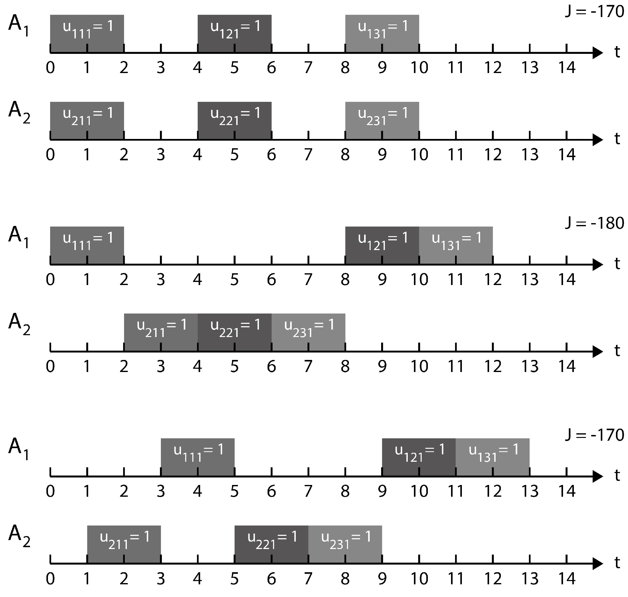
It can be seen that the difference between the functional Jp in (23) and the functional Job in the problem P is equal to losses caused by interruption of operation execution.
(c)
Let u p * ( t ) , ∀ t ∈ (T0, Tf] be an MS optimal program control in P and an allowable program control in Г; let x p * ( t ) be a solution of differential equations of the models M<o>, M<ν> subject to u ( t ) = u p * ( t ) . If so, then u p * ( t ) meets the requirements of the local section method (maximizes Hamilton’s function) for the problem Г. In this case, the vectors u p * ( t ) , x p * ( t ) return the minimum to the functional (1).
The scheme of computation can be stated as follows.
Step 1. An initial solution u g ( t ) , t ∈ (T0, Tf] (an arbitrary allowable control, in other words, allowable schedule) is selected. The variant u g ( t ) 0 is also possible.
Step 2. The main system of Equation (1) is integrated subject to h 0 ( x ( T 0 ) ) 0 and u ( t ) = u g ( t ) . The vector x ( o ) ( t ) is received as a result. In addition, if t = Tf, then the record value Jp = J p ( o ) can be calculated, and the transversality conditions (5) are evaluated.
Step 3. The adjoint system (2) is integrated subject to u ( t ) = u g ( t ) and (5) over the interval from t = Tf to t = T0. For time t = T0, the first approximation ψ i ( o ) ( T 0 ) is received as a result. Here the iteration number r = 0 is completed.
Step 4. From the point t = T0 onwards, the control u ( r + 1 ) ( t ) is determined (r = 0, 1, 2, … is the number of iteration) through the conditions (19). In parallel with the maximization of the Hamiltonian, the main system of equations and the adjoint system are integrated. The maximization involves the solving of several mathematical programming problems at each time point.
The branching of the problem Г occurs during the process of Hamiltonian maximization at some time t ˜ ∈ (T0, Tf] if the operation D æ ( i ) is being interrupted by the priority operation D ξ ( ω ) . In this case, the problem Г is split into two sub-problems ( Ρ æ ( i ) , Ρ ξ ( ω ) ).
Within the problem Ρ æ ( i ) , the operation D æ ( i ) is executed in an interrupt-disable mode. For other operations, this restriction is removed and the relaxed scheduling problem is solved via the method of successive approximations. Let us denote the received value of the goal function (23) by J p 0 ( 1 ) . Within the problem Ρ ξ ( ω ) , the previously started operation D æ ( i ) is terminated, and D ξ ( ω ) begins at time t ˜ . The resources released by the operation D æ ( i ) and not seized by D ξ ( ω ) can be used for other operations if any are present. Reallocation of resources should be performed according to (19). Subsequently, after completion of operation D ξ ( ω ) , the relaxed scheduling problem is solved. In this case, the value of the goal function (23) is denoted by J p 1 ( 1 ) . The record Jp is updated if J p 0 ( 1 ) < Jp or/and J p 1 ( 1 ) < J p ( 1 ) [we assume that the functional (23) is minimized]. If only J p 0 ( 1 ) < J p ( 1 ) , then Jp = J p 0 ( 1 ) . Similarly, if only J p 1 ( 1 ) < J p ( 1 ) , then Jp = J p 1 ( 1 ) . If both inequalities are true, then Jp = min{ J p 0 ( 1 ) , J p 1 ( 1 ) }. In the latter case, the conflict resolution is performed as follows: if J p 0 ( 1 ) < J p 1 ( 1 ) , then during the maximization of (19) D æ ( i ) is executed in an interrupt-disable mode. Otherwise, the operation D æ ( i ) is entered into the Hamiltonian at priority D ξ ( ω ) at arrival time t ˜ .
After conflict resolution, the allocation of resources is continued, complying with (19) and without interruption of operations until a new contention is similarly examined. The considered variant of dichotomous division in conflict resolution can be extended to the case of k ¯ -adic branching, where k ¯ is the number of interrupted operations at some time t ¯ .
The iterative process of the optimal schedule search is terminated under the following circumstances: either the allowable solution of the problem Г is determined during the solving of a relaxed problem or at the fourth step of the algorithm after the integration we receive:
| J p ( r + 1 ) J p ( r ) | < ε 1
where ε1 is a given value, r = 0, 1, … If the condition (24) is not satisfied, then the third step is repeated, etc.
The developed algorithm is similar to those considered in [20,37]. Here, the set of time points in which the Hamiltonian is to be maximized is formed on the previous iteration. These are points of operations interruption. Computational investigations of the proposed algorithm showed that the rate of convergence is predominantly influenced by the choice of the initial adjoint vector ψ ( t 0 ) . In its turn, ψ ( t 0 ) depends on the first allowable control that is produced at the first step. During the scheduling process, the machines are primarily assigned to operations of high dynamic priority.
To illustrate the main ideas of the algorithm, let us consider a simple example of a scheduling problem with two jobs, three operations, and a single machine, (T0, Tf] = (0, 14], a i æ ( o ) = 2 (I = 1,2; æ = 1, 2, 3); Θiæj(t) = 1 ∀ t; ε11(t) = 1 at t ∈ (0, 14], ε21(t) = 0 for 0 ≤ t < 1, ε21(t) = 1 for t ≥ 1. In this case, the model can be described as follows:
M = { u | x ˙ i æ ( o ) = ε i 1 u i æ 1 ( o ) ; z ˙ i æ 1 ( o , 1 ) = u i æ 1 ( o ) ; z ˙ i æ 1 ( o , 2 ) = z i æ 1 ( o , 1 ) ; z ˙ i æ 1 ( o , 3 ) = w i æ 1 ( o ) ; u i æ 1 ( o ) ( t ) , w i æ ( o ) ( t ) { 0 , 1 } , æ = 1 3 i = 1 2 u i æ 1 ( o ) ( t ) 1 ; u i 21 ( o ) ( a i 1 ( o ) x i 1 ( o ) ) = 0 ; u i 31 ( o ) ( a i 2 ( o ) x i 2 ( o ) ) = 0 ; w i æ 1 ( o ) ( a i æ ( o ) z i æ ( o , 1 ) ) = 0 ;   T 0 = 0 :   x i æ ( o ) ( t 0 ) = z i æ 1 ( o , 1 ) ( t 0 ) = z i æ 1 ( o , 2 ) ( t 0 ) = z i æ 1 ( o , 3 ) ( t 0 ) = 0 ;   T f = 14 :   x i æ ( o ) ( t f ) = 2 ; z i æ 1 ( o , l ) ( t f ) R 1 , l = 1 , 2 , 3 } .
The scheduling quality measure is defined by the expression:
J p = i = 1 2 æ = 1 3 [ ( a i æ ( o ) x i æ ( o ) ) 2 + ( z i æ 1 ( o , 1 ) z i æ 1 ( o , 3 ) + ( a i æ ( o ) ) 2 2 z i æ 1 ( o , 2 ) ) 2 ( z i æ 1 ( o , 1 ) ) 2 ] | t = T f i = 1 2 æ = 1 3 0 14 γ i æ ( τ ) u i æ 1 ( o ) ( τ ) d τ ,
where γiæ(t) are given time functions denoting the most preferable operation intervals: γ11 = 15γ+(6 − t), γ12 = 10γ+(9 − t), γ13 = 10γ+(11 − t), γ21 = 20γ+(8 − t), γ22 = 15γ+(8 − t), γ23 = 30γ+(11 − t). Here, γ+(α) = 1 if α ≥ 0 and γ+(α) = 0 if α < 0. The integration element in (27) can be interpreted similarly to previous formulas through penalties for operations beyond the bounds of the specified intervals. The scheduling problem can be formulated as follows: facilities-functioning schedule [control program u ( t ) ] returning a minimal value to the functional (27) under the conditions (26) and the condition of interruption prohibition should be determined.
The resulting schedule is shown in Figure 3.
The upper part of Figure 3 shows the initial feasible schedule implementing First-in-first-out processing. The second and third cases illustrate a conflict resolution for D 1 ( 1 ) interruption. The optimal schedule is presented in the third and the forth rows.

5. Qualitative and Quantitative Analysis of the MS Scheduling Problem

The representation of the scheduling problem in terms of a dynamic system (1) control problem allows applications of mathematical analysis tools from modern control theory (38,43,44).
For example, qualitative analysis based on control theory as applied to the dynamic system (1) provides the results listed in Table 1. This table confirms that our interdisciplinary approach to the description of MS OPC processes provides a fundamental base for MS problem decisions (or control and management) that have never been previously formalized and have high practical importance. The table also presents possible directions of practical implementation (interpretation) for these results in the real scheduling of communication with MS. For example, criteria for controllability and attainability in MS OPC problems can be used for MS control process verification for a given time interval.
The attainability sets (AS) of dynamic model (1) have an important place in qualitative analysis of MS control processes. These sets allow detailed analysis of computational procedures to two-point boundary problems with fixed ends of the state trajectory x ( t ) and a fixed time interval ( T 0 , T f ] .
An AS is a fundamental characteristic of any dynamic system. The AS approach determines a range of execution policies in the presence of disturbances over which the system can be guaranteed to meet certain goals. The union of these execution policies (i.e., feasible schedules) is called an AS in the state space. The union of possible performance outcomes from the given execution policies is called an AS in the performance space [43]. The AS in the state space depicts the possible states of a schedule subject to variations of the parameters (both planned and perturbation-driven) in the nodes and channels (e.g., different capacities, lot-sizes, etc.). Let us introduce the notation for an AS. D x ( t , T 0 , x ( T 0 ) , U ( x ( T 0 ) ) ) is an AS in the state space, D J ( t , T 0 , x ( T 0 ) , U ( x ( T 0 ) ) ) is an AS in the performance indicator’s space, and D ¯ J ξ ( t , T 0 , x ( T 0 ) , Ξ , U ( x ( T 0 ) ) ) is an approximated AS under disturbances at moment t. To interconnect schedule execution and performance analysis to the AS in the state space, an AS in the performance space can be brought into correspondence (see Figure 4).
In projecting these two ASs onto each other, a certain range of the schedule execution policies and the corresponding variation of the performance indicators can be determined. A continuous time representation allows investigation of the changes in execution at each time point. Therefore, at each time point, an AS can be calculated and related to output performance. The justification of the choice of the AS method is related to its dynamic nature ([43,44]). An AS may be favourable for obtaining estimations of performance attainability and consideration of the perturbations and attainability abilities of the schedules as time functions. In [13,19,33,34,35,36,37,38], we proposed different methods and algorithms of AS calculations. These results permit improvement of algorithm convergence in MS scheduling.
The proposed model interprets MS scheduling as a response to planning goal changes, demand fluctuations, and resource availability. In this interpretation, the problem is to schedule MS in order to achieve the planned goals (e.g., MS service level).
The model is scalable to other management levels of MS, i.e., orders and operations can be presented as MS configuration elements and orders, respectively. The transformation of parameters and goal criteria is also possible, i.e., the lead time can be considered as the MS cycle time. Hence, the MS strategic configuration and tactical planning can be optimized.
Let us analyse some particular features of the models (1) (see Figure 1). During the conducted experiments, it was revealed that the following model parameters influenced the improvement of the general quality index:
  • the total number of operations on a planning horizon;
  • a dispersion of volumes of operations;
  • a ratio of the total volume of operations to the number of processes;
  • a ratio of the amount of data of operation to the volume of the operation (relative operation density).
On the basis of the obtained etalon solutions, we can methodically justify the usage and quality of certain heuristics for certain variants of initial data (see Figure 5).
Having calculated optimal solutions for several points, it is possible to validate the decision to use either dynamic or heuristic planning algorithms. In Figure 4, the relative solution quality gained by the optimal control algorithm DYN is assumed to be 100%. The relative quality index of the heuristic solutions is calculated as a fraction of the optimal one, i.e., it can be observed that, in the case of a number of processes between 10 and 12, the quality of the heuristic and optimal solutions does not differ by more than 4%. In area 2, the DYN algorithm is preferable to the heuristics. If still using the heuristics, the FIFO algorithm is preferable to the Last-in-first-out one. The largest benefit from using the DYN algorithm is achieved in area 3. In this area, the LIFO algorithm is preferable to the FIFO algorithm.
Finally, the proposed model and algorithm allows for the achievement of better results in many cases in comparison with heuristics algorithms. However, this point is not the most important. The most important point is that this approach allows the interlinking of planning and scheduling models within an adaptation framework. Therefore, the suggested results are important in the Industry 4.0 domain. Hence, the proposed modeling complex does not exist as a “thing in itself” but works in the integrated decision-support system and guides the planning and scheduling decisions in dynamics on the principles of optimization and adaptation.

6. Conclusions

Optimal controls as functions of the system and control state allow for the generation of optimal decisions in consideration of a system’s evolution in time in the presence of perturbations which result in different system states. Optimal control approaches take another perspective as mathematical programming methods which represent schedules as trajectories.
Computational algorithms with regard to state, control, and conjunctive variable spaces exist in the literature. We have demonstrated that the advantages of optimal control methods are applicable to the treatment of large scale problems with complex constraints, the consideration of non-stationary process execution dynamics, the representation in differential equations of complex interrelations between process execution, capacity evolution, and machine setups. In addition, the advantages of optimal control also include accuracy of continuous time and accurate presentation of continuous flows (e.g., in process industry or energy systems) with the help of continuous state variables.
An important observation is that schedule presentation in terms of optimal control makes it possible to incorporate the rich variety of control theoretic axioms with regard to feedback adaptive control (mostly applied in the framework of production-inventory control models) as well as the use of control tools of qualitative performance analysis, such as attainable (reachable) sets. Limitations of control applications include conceptual and algorithmic restrictions such as continuous process applications and specific (i.e., non-generalized) forms of constructing algorithms with necessary requirements concerning optimality, convergence, and numerical stability.
In this study, we exemplified an application of optimal control to manufacturing scheduling. Fundamentally, this application dynamically decomposes the assignment matrix in time using differential equations, and then solves (by tendency) polynomial problems of small dimensionality at each point of time, with a subsequent integration of these partial solutions using the maximum principle by integrating main and adjoint equation systems. The small dimensionality at each point of time results from dynamic decomposition of job execution described by precedence relation constraints, i.e., at each point of time, we consider only operations that can be assigned to machines at this point of time, excluding those operations that already have been completed as well as those that cannot start because the predecessors have not yet been completed. Algorithmically, we solved these dimensionally small problems at subsequent point of times, integrate main and adjoint systems by the maximum principle, and considered how a particular assignment decision changes the schedule performance metric (e.g., tardiness). If an improvement is observed, the algorithm takes this assignment and moves further to next point of time and continues in this manner until Tf.
With regard to the limitations of this study, the schedule algorithm analysis by attainable sets was used to analyse the schedule outputs at the end of the planning horizon. At the same time, attainable sets (more precisely, their geometric approximations) can also be applied prior to schedule optimization to analyse if any feasible schedule exists for the given problem settings (resource capacities, etc.). This issue has not yet been considered.
In light of the revealed methodical shortcomings and application limitations of optimal control methods based on the maximum principle, the following future research avenues can be stated. First, concrete application cases need to be considered for which specific control models and algorithms will be developed. The construction of models and computational procedures within proved axioms of control theory is important. Second, application of qualitative performance analysis methods for control policy dynamic investigation under uncertainty, such as attainable sets, must be named. These tools might be helpful with regard to an analysis of production schedule robustness, supply chain resilience, and Industry 4.0 system flexibility. Third, computational methods themselves require further investigation and modification for concrete application cases. Therefore, a closer collaboration between control and industrial engineers is critical for future applications of control methods in operations and future supply chain management.

Author Contributions

Boris Sokolov and Dmitry Ivanov conceived and designed the experiments; Boris Sokolov performed the experiments; Alexandre Dolgui and Boris Sokolov analyzed the data; Alexandre Dolgui and Dmitry Ivanov contributed reagents/materials/analysis tools; all authors wrote the paper.

Acknowledgments

The research described in this paper is partially supported by the Russian Foundation for Basic Research (grants 16-07-00779, 16-08-00510, 16-08-01277, 16-29-09482-оfi-i, 17-08-00797, 17-06-00108, 17-01-00139, 17-20-01214, 17-29-07073-оfi-i, 18-07-01272, 18-08-01505), grant 074-U01 (ITMO University), state order of the Ministry of Education and Science of the Russian Federation No. 2.3135.2017/4.6, state research 0073-2018-0003, International project ERASMUS +, Capacity building in higher education, No. 73751-EPP-1-2016-1-DE-EPPKA2-CBHE-JP, Innovative teaching and learning strategies in open modelling and simulation environment for student-centered engineering education.

Conflicts of Interest

The authors declare no conflict of interest.

Abbreviations

ASAttainability Sets
OPCOptimal Program Control
MSManufacturing System
SSAMSuccessive Approximations Method

Appendix A. List of Notations

x is a vector of the MS general state
u is a vector of the generalized control
h 0 , h 1 are known vector function that are used for the state x and conditions
q ( 1 ) , q ( 2 ) are known spatio-temporal, technical and technological constraints
J ϑ are indicators characterizing MS schedule quality
ξ is a known vector-function of perturbation influences
ψ is a vector of conjugate system state
Η is a Hamilton’s function
J o b is a scalar form of the vector quality measure
M g is a dynamic model of MS motion control,
M k is a dynamic model of MS channel control,
M o is a dynamic model of MS operational control,
Mf is a dynamic model of MS flow control,
Mp is a dynamic model of MS resource control,
M e is a dynamic model of MS operation parameters control,
M c is a dynamic model of MS structure dynamic control,
M ν is a dynamic model of MS auxiliary operation control,
t is a current value of time,
T 0 is start instant of time of the planning (scheduling) horizon,
T f is end instant of time of the planning (scheduling) horizon,
ψ l is a component of adjoint vector ψ ( t ) ,
x l is an element of a general vector x ( t ) ,
λ α ( t ) is a dynamic Lagrange multiplier which corresponds to the components of vector q α ( 1 ) ,
ρ β ( t ) is a dynamic Lagrange multiplier which is corresponds to the components of vector q α ( 2 ) ,
z i j μ ( o ) is an auxiliary variable which characterizes the execution of the operation
α is a current number of constraints q α ( 1 ) ,
β is a current number of constraints q α ( 2 ) ,
ψ l ( T 0 ) is a component of adjoint vector ψ ( t ) at the moment t = T 0 ,
ψ l ( T f ) is a component of adjoint vector ψ ( t ) at the moment t = T f ,
H ( x ( t ) , u ( t ) , ψ ( t ) ) = Ψ T f ( x , u , t ) is a Hamilton’s function,
Φ ( ψ ( T 0 ) ) is an implicit function of boundary condition,
a is a vector given quantity value which corresponds to the vector x ( t ) ,
Δ u is a function of boundary conditions,
ρ ( T f ) is a discrepancy of boudary conditions,
ψ ( r ) ( T 0 ) is a vector of adjoint system at the moment, t = T 0
r is a current number of iteration during schedule optimization,
Π ˜ is a derivative matrix,
ε u is a given accuracy of Newton’s method iterative procedure,
C i is a penalty coefficient,
Δ < i , ( r 1 ) > is a component of the function Δ ( r 1 ) gradient on the iteration r 1 ,
γ < i , r > is a step of gradient (subgradient) method (algorithm) on the iteration r
ψ ˜ ˜ ( 0 ) ( T 0 ) is a adjoint vector at the moment t = T 0 on the iteration 0 ,
ψ ˜ ( r ) ( T 0 ) is a adjoint vector at the moment t = T 0 on the iteration r ,
σ′ is a some part of the interval σ = ( T 0 , T f ] ,
N ˜ ˜ is a assumed operator of new approximation procedure,
t ˜ < e , ( r + 1 ) > , t ˜ < e , ( r + 1 ) > are time moments of operation interruption,
u p * ( t ) is a vector of generalized control in relaxed problem of MS OPC construction,
x p * ( t ) is a vector of general state in relaxed problem of MS OPC construction,
u g ( t ) is a vector of an arbitrary allowable control (allowable schedule),
D æ ( i ) is a operation æ with object i ,
D ξ ( ω ) is a operation ξ with object ω ,
Ρ æ ( i ) , Ρ ξ ( ω ) is a current number of the branch and bound method subproblems,
J p 0 ( 1 ) is a value of scalar form of MS vector quality measure for the first subproblem,
J p 1 ( 1 ) is a value of scalar form of MS vector quality measure for the second subproblem,
D x is an attainable set,
ϑ is a current index of MS control model,
g is an index of MS motion control model,
k is an index of MS channel control model,
o is an index of MS operation control model,
f is an index of MS flow control model,
p is an index of MS resource control model,
e is an index of MS operation parameters control model,
c is an index of MS structure dynamic control model,
ν is an index of MS auxiliary operation control model,
l is a current number of MS elements and subsystems,
u is a scalar allowable control input,
Θ is a current number of model,
æ is a number of operation æ , ξ is a number of operation ξ , ω is a number of operation ω ,
i is a current number of external object (customer),
j is a current number of internal object resource,
ε 1 , ε 2 are known constants which characterize the accuracy of iterative solution of boundary-value problem.
δ ˜ is a step of integration

References

  1. Blazewicz, J.; Ecker, K.; Pesch, E.; Schmidt, G.; Weglarz, J. Scheduling Computer and Manufacturing Processes, 2nd ed.; Springer: Berlin, Germany, 2001. [Google Scholar]
  2. Pinedo, M. Scheduling: Theory, Algorithms, and Systems; Springer: New York, NY, USA, 2008. [Google Scholar]
  3. Dolgui, A.; Proth, J.-M. Supply Chains Engineering: Useful Methods and Techniques; Springer: Berlin, Germany, 2010. [Google Scholar]
  4. Werner, F.; Sotskov, Y. (Eds.) Sequencing and Scheduling with Inaccurate Data; Nova Publishers: New York, NY, USA, 2014. [Google Scholar]
  5. Lauff, V.; Werner, F. On the Complexity and Some Properties of Multi-Stage Scheduling Problems with Earliness and Tardiness Penalties. Comput. Oper. Res. 2004, 31, 317–345. [Google Scholar] [CrossRef]
  6. Jungwattanakit, J.; Reodecha, M.; Chaovalitwongse, P.; Werner, F. A comparison of scheduling algorithms for flexible flow shop problems with unrelated parallel machines, setup times, and dual criteria. Comput. Oper. Res. 2009, 36, 358–378. [Google Scholar] [CrossRef]
  7. Dolgui, A.; Kovalev, S. Min-Max and Min-Max Regret Approaches to Minimum Cost Tools Selection 4OR-Q. J. Oper. Res. 2012, 10, 181–192. [Google Scholar] [CrossRef]
  8. Dolgui, A.; Kovalev, S. Scenario Based Robust Line Balancing: Computational Complexity. Discret. Appl. Math. 2012, 160, 1955–1963. [Google Scholar] [CrossRef]
  9. Sotskov, Y.N.; Lai, T.-C.; Werner, F. Measures of Problem Uncertainty for Scheduling with Interval Processing Times. OR Spectr. 2013, 35, 659–689. [Google Scholar] [CrossRef]
  10. Choi, T.-M.; Yeung, W.-K.; Cheng, T.C.E. Scheduling and co-ordination of multi-suppliers single-warehouse-operator single-manufacturer supply chains with variable production rates and storage costs. Int. J. Prod. Res. 2013, 51, 2593–2601. [Google Scholar] [CrossRef]
  11. Harjunkoski, I.; Maravelias, C.T.; Bongers, P.; Castro, P.M.; Engell, S.; Grossmann, I.E.; Hooker, J.; Méndez, C.; Sand, G.; Wassick, J. Scope for industrial applications of production scheduling models and solution methods. Comput. Chem. Eng. 2014, 62, 161–193. [Google Scholar] [CrossRef]
  12. Bożek, A.; Wysocki, M. Flexible Job Shop with Continuous Material Flow. Int. J. Prod. Res. 2015, 53, 1273–1290. [Google Scholar] [CrossRef]
  13. Ivanov, D.; Dolgui, A.; Sokolov, B. Robust dynamic schedule coordination control in the supply chain. Comput. Ind. Eng. 2016, 94, 18–31. [Google Scholar] [CrossRef] [Green Version]
  14. Giglio, D. Optimal control strategies for single-machine family scheduling with sequence-dependent batch setup and controllable processing times. J. Sched. 2015, 18, 525–543. [Google Scholar] [CrossRef]
  15. Lou, S.X.C.; Van Ryzin, G. Optimal control rules for scheduling job shops. Ann. Oper. Res. 1967, 17, 233–248. [Google Scholar] [CrossRef]
  16. Maimon, O.; Khmelnitsky, E.; Kogan, K. Optimal Flow Control in Manufacturing Systems; Springer: Berlin, Germany, 1998. [Google Scholar]
  17. Ivanov, D.; Sokolov, B. Dynamic coordinated scheduling in the manufacturing system under a process modernization. Int. J. Prod. Res. 2013, 51, 2680–2697. [Google Scholar] [CrossRef]
  18. Pinha, D.; Ahluwalia, R.; Carvalho, A. Parallel Mode Schedule Generation Scheme. In Proceedings of the 15th IFAC Symposium on Information Control Problems in Manufacturing INCOM, Ottawa, ON, Canada, 11–13 May 2015. [Google Scholar]
  19. Ivanov, D.; Sokolov, B. Structure dynamics control approach to supply chain planning and adaptation. Int. J. Prod. Res. 2012, 50, 6133–6149. [Google Scholar] [CrossRef]
  20. Ivanov, D.; Sokolov, B.; Dolgui, A. Multi-stage supply chains scheduling in petrochemistry with non-preemptive operations and execution control. Int. J. Prod. Res. 2014, 52, 4059–4077. [Google Scholar] [CrossRef]
  21. Pontryagin, L.S.; Boltyanskiy, V.G.; Gamkrelidze, R.V.; Mishchenko, E.F. The Mathematical Theory of Optimal Processes; Pergamon Press: Oxford, UK, 1964. [Google Scholar]
  22. Athaus, M.; Falb, P.L. Optimal Control: An Introduction to the Theory and Its Applications; McGraw-Hill: New York, NY, USA; San Francisco, CA, USA, 1966. [Google Scholar]
  23. Lee, E.B.; Markus, L. Foundations of Optimal Control Theory; Wiley & Sons: New York, NY, USA, 1967. [Google Scholar]
  24. Moiseev, N.N. Element of the Optimal Systems Theory; Nauka: Moscow, Russia, 1974. (In Russian) [Google Scholar]
  25. Bryson, A.E.; Ho, Y.-C. Applied Optimal Control; Hemisphere: Washington, DC, USA, 1975. [Google Scholar]
  26. Gershwin, S.B. Manufacturing Systems Engineering; PTR Prentice Hall: Englewood Cliffs, NJ, USA, 1994. [Google Scholar]
  27. Sethi, S.P.; Thompson, G.L. Optimal Control Theory: Applications to Management Science and Economics, 2nd ed.; Springer: Berlin, Germany, 2000. [Google Scholar]
  28. Dolgui, A.; Ivanov, D.; Sethi, S.; Sokolov, B. Scheduling in production, supply chain Industry 4.0 systems by optimal control: fundamentals, state-of-the-art, and applications. Int. J. Prod. Res. 2018. forthcoming. [Google Scholar]
  29. Bellmann, R. Adaptive Control Processes: A Guided Tour; Princeton University Press: Princeton, NJ, USA, 1972. [Google Scholar]
  30. Maccarthy, B.L.; Liu, J. Addressing the gap in scheduling research: A review of optimization and heuristic methods in production scheduling. Int. J. Prod. Res. 1993, 31, 59–79. [Google Scholar] [CrossRef]
  31. Sarimveis, H.; Patrinos, P.; Tarantilis, C.D.; Kiranoudis, C.T. Dynamic modeling and control of supply chains systems: A review. Comput. Oper. Res. 2008, 35, 3530–3561. [Google Scholar] [CrossRef]
  32. Ivanov, D.; Sokolov, B. Dynamic supply chains scheduling. J. Sched. 2012, 15, 201–216. [Google Scholar] [CrossRef]
  33. Ivanov, D.; Sokolov, B. Adaptive Supply Chain Management; Springer: London, UK, 2010. [Google Scholar]
  34. Ivanov, D.; Sokolov, B.; Käschel, J. Integrated supply chain planning based on a combined application of operations research and optimal control. Central. Eur. J. Oper. Res. 2011, 19, 219–317. [Google Scholar] [CrossRef]
  35. Ivanov, D.; Dolgui, A.; Sokolov, B.; Werner, F. Schedule robustness analysis with the help of attainable sets in continuous flow problem under capacity disruptions. Int. J. Prod. Res. 2016, 54, 3397–3413. [Google Scholar] [CrossRef]
  36. Kalinin, V.N.; Sokolov, B.V. Optimal planning of the process of interaction of moving operating objects. Int. J. Differ. Equ. 1985, 21, 502–506. [Google Scholar]
  37. Kalinin, V.N.; Sokolov, B.V. A dynamic model and an optimal scheduling algorithm for activities with bans of interrupts. Autom. Remote Control 1987, 48, 88–94. [Google Scholar]
  38. Ohtilev, M.Y.; Sokolov, B.V.; Yusupov, R.M. Intellectual Technologies for Monitoring and Control of Structure-Dynamics of Complex Technical Objects; Nauka: Moscow, Russia, 2006. [Google Scholar]
  39. Krylov, I.A.; Chernousko, F.L. An algorithm for the method of successive approximations in optimal control problems. USSR Comput. Math. Math. Phys. 1972, 12, 14–34. [Google Scholar] [CrossRef]
  40. Chernousko, F.L.; Lyubushin, A.A. Method of successive approximations for solution of optimal control problems. Optim. Control Appl. Methods 1982, 3, 101–114. [Google Scholar] [CrossRef]
  41. Ivanov, D.; Sokolov, B.; Dolgui, A.; Werner, F.; Ivanova, M. A dynamic model and an algorithm for short-term supply chain scheduling in the smart factory Industry 4.0. Int. J. Prod. Res. 2016, 54, 386–402. [Google Scholar] [CrossRef]
  42. Hartl, R.F.; Sethi, S.P.; Vickson, R.G. A survey of the maximum principles for optimal control problems with state constraints. SIAM Rev. 1995, 37, 181–218. [Google Scholar] [CrossRef]
  43. Chernousko, F.L. State Estimation of Dynamic Systems; Nauka: Moscow, Russia, 1994. [Google Scholar]
  44. Gubarev, V.A.; Zakharov, V.V.; Kovalenko, A.N. Introduction to Systems Analysis; LGU: Leningrad, Russia, 1988. [Google Scholar]
Figure 1. The scheme of optimal program control model interconnection.
Algorithms 11 00057 g001
Figure 2. Optimal control computational methods.
Algorithms 11 00057 g002
Figure 3. Optimal schedule results.
Algorithms 11 00057 g003
Figure 4. Representation of dynamic changes in schedule performance by attainable sets.
Algorithms 11 00057 g004
Figure 5. Comparison of heuristic algorithms’ quality.
Algorithms 11 00057 g005
Table 1. Application of optimal control approaches to scheduling.
Results and Their ImplementationThe Main Results of Qualitative Analysis of MS Control ProcessesThe Directions of Practical Implementation of the Results
No
1Analysis of solution existence in the problems of MS controlAdequacy analysis of the control processes description in control models
2Conditions of controllability and attainability in the problems of MS controlAnalysis MS control technology realizability on the planning interval. Detection of main factors of MS goal and information-technology abilities.
3Uniqueness condition for optimal program controls in scheduling problemsAnalysis of possibility of optimal schedules obtaining for MS functioning
4Necessary and sufficient conditions of optimality in MS control problemsPreliminary analysis of optimal control structure, obtaining of main expressions for MS scheduling algorithms
5Conditions of reliability and sensitivity in MS control problemsEvaluation of reliability and sensitivity of MS control processes with respect to perturbation impacts and to the alteration of input data contents and structure

