A Heuristic Approach to Solving the Train Traffic Re-Scheduling Problem in Real Time

Abstract

Effectiveness in managing disturbances and disruptions in railway traffic networks, when they inevitably do occur, is a significant challenge, both from a practical and theoretical perspective. In this paper, we propose a heuristic approach for solving the real-time train traffic re-scheduling problem. This problem is here interpreted as a blocking job-shop scheduling problem, and a hybrid of the mixed graph and alternative graph is used for modelling the infrastructure and traffic dynamics on a mesoscopic level. A heuristic algorithm is developed and applied to resolve the conflicts by re-timing, re-ordering, and locally re-routing the trains. A part of the Southern Swedish railway network from Karlskrona centre to Malmö city is considered for an experimental performance assessment of the approach. The network consists of 290 block sections, and for a one-hour time horizon with around 80 active trains, the algorithm generates a solution in less than ten seconds. A benchmark with the corresponding mixed-integer program formulation, solved by commercial state-of-the-art solver Gurobi, is also conducted to assess the optimality of the generated solutions.

1. Introduction

The definitions of “system performance” and “quality of service” in railway traffic and transportation vary, but more recent reports, e.g., from the Boston Consultancy Group [1] and the European Commission [2], indicate that many European countries face challenges with regard to the reliability and punctuality of rail services. Several different factors contribute to these challenges, where the frequency and magnitude of disruptions and disturbances is one factor. The effectiveness in managing the disturbances and disruptions in railway traffic networks when they inevitably do occur is another aspect to consider. In this paper, we focus on the latter, and more specifically, on the problem of real-time train traffic re-scheduling, also referred to as train dispatching [3].

In general, the problem of re-scheduling train traffic in real-time is known to be a hard problem to solve by expert traffic dispatchers in practice, as well as by state-of-the-art scheduling software. There is thus often a trade-off that needs to be made regarding permitted computation time and expected solution quality. Heuristic approaches, or approaches based on, e.g., discrete-event simulation, are often rather quick, since they work in a greedy manner, but sometimes they fail to deliver a reasonable solution or even end up in deadlock. Exact approaches, based on, e.g., mixed-integer programming models solved by branch-and-cut algorithms are, on the other hand, less greedy, but can be very time-consuming, especially if the search space is large, and suffer from significant redundancy. Another aspect concerns the selected level of granularity of the traffic and infrastructure model, and this may indirectly affect the computation time and the quality of the solution as well.

Over the latest three decades, a variety of algorithms and methods have been proposed to solve the train traffic re-scheduling (or, train dispatching) problem, see [3,4,5,6] for more recent surveys. These previously proposed approaches have different strengths and limitations, depending on the intended application and context in mind. In Section 2, we provide a more comprehensive summary of state-of-the-art methods addressing this problem.

In this paper, we propose a heuristic approach to solve the real-time train traffic re-scheduling problem. We view the problem as a blocking/no-wait, parallel-machine job-shop scheduling problem [3]. A job corresponds to a train’s path along a pre-determined sequence of track sections (i.e., machines). Each part of that path corresponds to an operation. “blocking/no-wait” constraint refers to that there is no possibility to finish an operation if the next operation of the same job cannot get access to the required machine for processing, i.e. there is no storage space between machines that allows jobs and their current operation to wait for an occupied machine to become available. That is, when an operation of a job is completed, the next operation of that job must immediately start. This corresponds to the train needing at all times to have explicit access to a track section (independent of whether the train is moving or waiting). This problem is here modeled as a graph, where the graph is a hybrid between a mixed graph and an alternative graph. The benefit of using a hybrid graph is the possibility of reducing the number of required computations when constructing the graph. The problem is then solved by a heuristic algorithm. The proposed mixed graph model is discussed in Section 3, and the proposed heuristic algorithm is presented in detail in Section 4. The performance of the proposed approach is assessed in an experimental study, where the approach has been applied to solve a number of disturbance scenarios for a dense part of the Swedish southern railway network system. The performance assessment also includes a benchmark with the commercial optimization software Gurobi (v 6.5.1), using the corresponding mixed integer programming (MIP) model (which is presented in Appendix A). This experimental study is presented in Section 5. Section 6 presents some conclusions from the experimental study and provides pointers to future work.

2. Related Work

Szpigel [7] was, in 1973, one of the pioneers, adapting the job-shop scheduling (JSS) problem formulation for the train scheduling problem. This was later developed by other researchers such as D’Ariano et al. [8], Khosravi et al. [9], Liu and Kozan [10], Mascis and Pacciarelli [11], and Oliveira and Smith [12].

The JSS paradigm is also explored in the mixed-integer linear programming (MILP) approach proposed by Törnquist Krasemann and Persson in 2007 [13], where the primary focus was on creating and evaluating strategies for reducing the search space via model re-formulations. Different problem formulations were experimentally evaluated in several disturbance scenarios occurring on a double-tracked network with bi-directional traffic, and solved by commercial software for a time horizon of 60–90 min. The effectiveness of the approach and the different strategies were shown to be highly dependent on the size of the problem and type of disturbance.

A heuristic approach based on a MILP formulation was also proposed in [14]. A time horizon of 30 to 60 min was defined for testing the disturbing scenarios. The commercial solver CPLEX was used to solve the problem, with an allowed computation time of 180 s. Significant effort was made to tune the heuristic algorithm, and the results were compared with exact ones. For up to a 40 min time horizon, the algorithm generated good results.

A MIP model was also applied on a double-track railway corridor, where the focus is on local re-routing of trains to allow for bi-directional traffic and special constraints to respect the safety requirements [15].

As already mentioned, the real-time train traffic re-scheduling problem is a hard problem to solve. This is often an effect of the large solution space, which may be difficult to efficiently navigate in due to significant redundancy. That is, depending on the problem formulation and selected objective function, particularly, optimization solvers may find multiple equally good solutions and also have difficulties finding strong bounds. Finding optimal, or near-optimal, solutions may thus be very time-consuming.

In order to reduce the computational time, one can partition the problem into a set of different sub-problems and solve them in parallel, in a distributed manner with some sort of coordination mechanism. The partitioning can be done in space (i.e., by dividing the infrastructure, or the associated constraints, into separate parts), or in time (i.e., rolling-time horizon). Corman et al. [16,17,18] proposed and benchmarked a centralized and a distributed re-scheduling approach for the management of a part of the Dutch railway network based on a branch-and-bound approach. These variations come from various static and dynamic priorities that are considered for scheduling. They also worked on a coordination system between multiple dispatching areas. The aim was to achieve a globally optimal solution by combining local solutions. Some constraints are defined for the border area and a branch-and-bound algorithm solves the coordinator problem.

Another approach for reducing the complexity of the problem is to use classical decomposition techniques, which are becoming more frequently used to overcome the complexity (and the associated long computation times) of the train re-scheduling problem when using exact approaches. Lamorgese and Mannino proposed an exact method, which decomposes and solves the problem with a master-slave procedure using column generation [19]. The master is associated with the line traffic control problem and the slaves with the station traffic control.

Decomposition has also been used to reduce the complexity of the associated MIP model of the train re-scheduling problem [20]. An iterative Lagrangian relaxation algorithm is used to solve the problem.

Tormo et al. [21] have investigated different disturbance management methods, for the purpose of supporting railway dispatchers with the assessment of the appropriateness of each method for different problems in the railway operations. They categorized the disturbance management approaches into three subcategories. The first one is to minimize the overall delays at the network level. The second one is the evaluation of disturbances based on the severity, and the third one is to assume the equal importance of each incident. An incremental heuristic method has been compared with a two-phase heuristic approach in [22]. At each processing step, partial resource allocation and partial scheduling are repeated until a complete solution is generated. In a two-phase heuristic approach, the algorithm creates the routes for all the trains with a complete labelling procedure in phase one, and then solves the problem with an approximation algorithm in phase two.

The use of task parallelization to reduce computation time was explored by Bettinelli et al. [23], who proposed a parallel algorithm for the train scheduling problem. The problem is modelled by a graph. For conflict resolution, some dispatching rules are applied. The algorithm solves the problem in an iterative, greedy manner, and to decrease the computational time, the tasks are parallelized. The algorithm enhances the quality of the solutions using neighbourhood search and tabu search. The neighbourhood search has a significant impact on the quality of generated solutions, according to the authors.

Another interesting study of different approaches to variable neighbourhood search and quality assessment is available in [24]. Local search techniques are also used in [25], where the problem is modeled as a hybrid job-shop scheduling problem.

In [10], the train scheduling problem is formulated as a blocking parallel-machine job-shop scheduling problem and modeled as an alternative graph. A heuristic algorithm, referred to as “the feasibility satisfaction procedure”, is proposed to resolve the conflicts. The model attempts to consider train length, upgrading the track sections, increasing the trains’ speed on the identified tardy section and shortening the local runtime of each train on bottleneck sections. The application was designed for the train scheduling problem and is not considering re-scheduling. In the first step, the problem is solved by a shifting bottleneck algorithm without considering the blocking condition. In the next step, the blocking condition is satisfied by using an alternative graph model.

Khosravi et al. [9] also address the train scheduling and re-scheduling problem using a job-shop scheduling problem formulation, and the problem is solved using a shifting bottleneck approach. Decomposition is used to convert the problem into several single-machine problems. Different variations of the method are considered for solving the single-machine problems. The algorithm benefits from re-timing and re-ordering trains, but no re-routing of trains is performed.

A job-shop scheduling approach is also used to insert additional trains to an existing timetable without introducing significant consecutive delays to the already-scheduled trains [26]. A branch and bound algorithm and an iterative re-ordering strategy are proposed to solve this problem in real-time. Re-timing and re-ordering are conducted in a greedy manner. They have suggested a new bound for the branch and bound algorithm and an iterative re-ordering algorithm, which helps to find solutions in an acceptable computational time.

The main challenge in this study is to—inspired by previous promising research work—develop, apply and evaluate an effective algorithm that, within 10 s, can find sufficiently good solutions to a number of different types of relevant disturbance scenarios for a medium-sized sub-network and a time horizon of 60–90 min. A hybrid of the mixed graph and alternative graph (a derivation of the disjunctive graph, which satisfies the blocking constraint [11]) formulation is used for modelling the train traffic re-scheduling problem. This graph allows us to model the problem with a minimum number of arcs, which is expected to improve the efficiency of the algorithm. The model of the infrastructure and traffic dynamics is on the mesoscopic level, which considers block sections, clear time and headway distance, based on static parameter values. A heuristic algorithm is developed for conflict resolution. This algorithm is an extension of the algorithm developed by Gholami and Sotskov for hybrid job-shop scheduling problems [27]. The extended algorithm provides an effective strategy for visiting the conflicting operations and the algorithm makes use of re-timing, re-ordering, and local re-routing of trains while minimizing train delays.

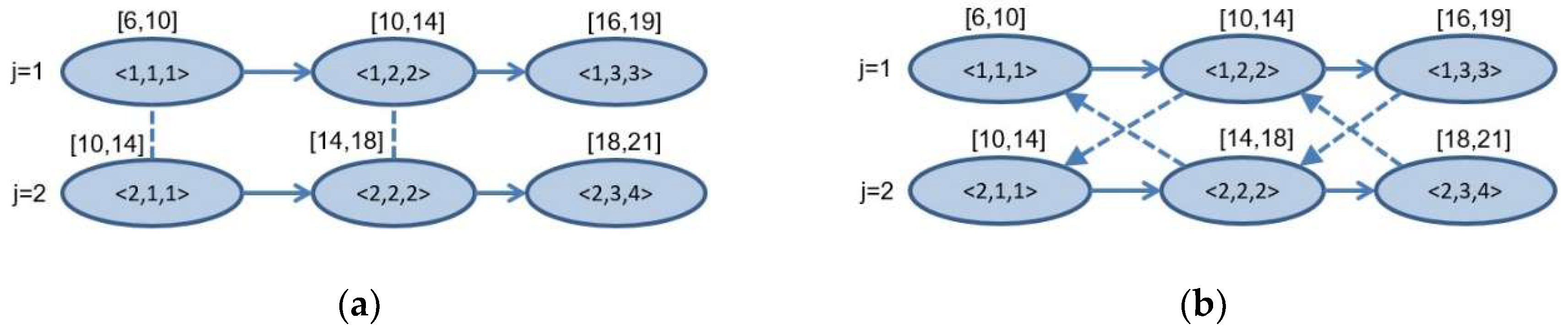
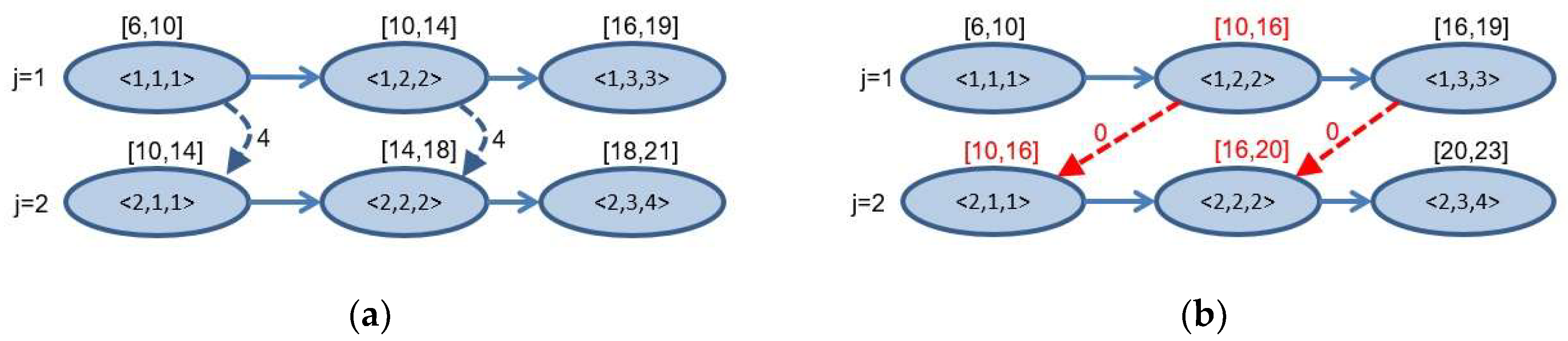
3. Modelling the Job-Shop Scheduling Problem Using a Graph

A well-known and efficient way of modelling the job-shop scheduling problem is to use graphs. Graph theory is a well-studied area in the computational sciences, and it provides efficient algorithms and data structures for implementation. These features make the graph a suitable candidate for modeling the problem addressed in this paper.

In a job-shop scheduling problem, there are $n$ jobs that have to be served by $m$ different types of machines. Each job $j\in J$ has its own sequence of operations $O_j=\left\{o_{j,1},o_{j,2},\dots ,o_{j,m}\right\}$ to be served by different predefined machines from the set $M$. The jobs have to be served by machines exclusively. The job-shop scheduling problem can be formulated using a mixed graph model $G=\left(O,C,D\right)$, or equivalently by a disjunctive graph model. Let $O$ denote the set of all operations to be executed by a set of different machines $M$. The set $C$ represents a predefined sequence of operations for each job $j$ to visit machines from the set $M$. The two operations $o_{j,i}$ and $o_{j\prime ,i\prime }$ which have to be executed on the same machine $m\in M$, cannot be processed simultaneously. This restriction is modelled by an edge $\left[o_{j,i},o_{j\prime ,i\prime }\right]\in D$ (if a mixed graph is used) or equivalently by pairs of disjunctive arcs $\{\left(o_{j,i},o_{j\prime ,i\prime }\right),$ and $\left(o_{j\prime ,i\prime },o_{j,i}\right)$ } (if a disjunctive graph is used). In this paper, the mixed graph is used for modelling the primary state of the problem. Two vertices, $o_s$ and $o_d$ as the source and destination vertices, respectively, are added to the model to transform it to a directed acyclic graph.

Using the terms “arc” and “edge” may be confusing. Edges may be directed or undirected; undirected edges are also called “lines”, and directed edges are called “arcs” or “arrows”. In this paper, the term “edge” is used for undirected edges, and the term “arc” is used for directed edges.

To serve the operations in a job-shop scheduling problem, only one instance of each machine of type $m$ is available. In a hybrid job-shop as a derivation of the job-shop scheduling problem, a set $M_m$ ($\left|M_m\right|\ge 1$ ) is available to serve the operations [28]. The notation $\langle m,u\rangle$ is used to indicate a specific machine or resource $u$ from a set $M_m$ if it is necessary. These uniform parallel machine sets increase the throughput and provide more flexibility in the scheduling process.

A train is here synonymous with a job in the job-shop scheduling problem. A train route from the source station to the destination can be considered to be a sequence of operations for a job $j$. Each railroad section is synonymous to a machine $m$. In

Table 1. The notations used for sets, indices, parameters, and variables.

Sets and Indices	Description
$M$	Set of all railway sections (i.e., machines).
$m$	The index used to denote a specific section in the set$M$.
$M_m$	The sub-set of tracks and platforms that belongs to section $m$. (i.e., parallel machines)
$m,u$	A track/platform/resource instance number$u$ from a set$M_m$.
$J$	Set of all trains (i.e., jobs).
$j$	The index used to denote a specific train.
$O$	Set of all train events (i.e., operations).
$O_j$	Set of all events that belong to train $j$.
$O^m$	Set of all events to be scheduled on a section $m$.
$O^{m,u}$	Set of all events to be scheduled on track $u$ of section$m$.
$i$	The index used to denote a specific train event$i$.
$o_{j,i}$	The symbol used to denote the event $i$ which belongs to train$j$.
$\langle j,i,m,u\rangle$	Tuple which refers to train $j$ and its event $i$ which occurs in section$m$ and scheduled for track $u$. When the section is single line $u$ will be ignored.
$(\prime )$	Prime symbol used to distinguish between two instances (i.e., job $j$ and $j^{\prime }$ ).
Parameters	Description
$c_m$	The required minimum clear time that must pass after a train has released the assigned track $u$ of section$m$ and before another train may enter track $u$ of section$m$.
$h_m$	The minimum headway time distance that is required between trains (head-head and tail-tail) that run in sequence on the same track $u$ of section$m$.
$d_{j,i}$	The minimum running time, or dwell time, of event$i$ that belongs to train$j$.
$b_{j,i}^{initial}$	This parameter specifies the initial starting time of event $i$ that belongs to train$j$.
$e_{j,i}^{initial}$	This parameter specifies the initial completion time of event $i$ that belongs to train$j$.
$p{s}_{j,i}$	This parameter indicates if event $i$ includes a planned stop at the associated segment.
Variables	Description
$x_{j,i}^{begin}$	The re-scheduled starting time of event $i$ that belongs to train$j$.
$x_{j,i}^{end}$	The re-scheduled completion time of event $i$ that belongs to train$j$ .
$t_{j,i}$	The tardiness (i.e., delay for train $j$ to complete event$i$ ).
$z_{j,i}$	Delay of even$\mathrm{t}$ $i,i\in O$, exceeding µ time units, which is set to three minutes here.
$q_{j,i,u}$	A binary variable which is 1, if the event $i$ uses track $u$.
${\gamma }_{j,i,j\prime ,i\prime }$	A binary variable which is 1, if the event $i$ occurs before event$i\prime$.
${\lambda }_{j,i,j\prime ,i\prime }$	A binary variable which is 1, if the event $i$ is rescheduled to occur after event$i\prime$.
$bu{f}_{j,i}$	Remaining buffer time for train $j$ to complete an event$\langle j,i\rangle$.
$TF{D}_j$	The delay for train $j$ once it reaches its final destination, i.e., $t_{j,last}$ which corresponds to the delay when completing its last event.

, below, we introduce the notations that are used to describe and define the hybrid graph model, algorithmic approach, and corresponding MIP model.

To solve the job-shop scheduling problem modelled by a graph, for every two conflicting operations the algorithm is responsible for determining the best execution order to reduce the objective function value. A potential conflict occurs when for two events$o_{j,i}$, and$o_{j\prime ,i\prime }$ belonging to jobs $j$ and $j\prime$ respectively, the following criteria become true:

$$x_{j,i}^{begin}<x_{j\prime ,i\prime }^{begin}\mathrm{and}{x}_{j\prime ,i\prime }^{end}\le x_{j,i}^{begin}+d_{j\prime ,i\prime }$$

(1)

The algorithm is in charge of replacing the set of edges $D$ with a subset of arcs $D^{\prime }$, which defines the order to be served by a resource. As a result, the set of edges $D$ will be substituted by a selected subset of directed arcs$D^{\prime }$, and the mixed graph $G=\left(O,C,D\right)$ will be transformed into a digraph$G^{\prime }=\left(O,C{{\displaystyle \cup }}^{\text{}}{D}^{\prime },\varnothing \right)$.

In this paper, a multi-track railway traffic network will be considered as a job-shop scheduling problem with parallel machines (hybrid job-shop) at each stage.

4. A Heuristic Algorithm for Conflict Resolution in the Mixed Graph $G$

When a disturbance occurs, a graph $G$ has to be generated from the ongoing and remaining events for all the trains within the predefined time horizon. Later, the algorithm has to resolve the conflicts between trains affected by disturbance and potential knock-on effects. To resolve all the conflicts in a graph$G$, the algorithm has to visit all conflict pairs, and by replacing the edges with directed arcs, clarify the priorities for using the resources (i.e., the sections and associated tracks). In this research, the objective is to minimize the sum of the total final delay that each train experiences at its final destination (i.e., $TF{D}_j=Max\left(0,x_{j,last}^{end}-e_{j,last}^{initial}\right),j\in J$ ). We also measure the corresponding when the delay threshold is three minutes, i.e., only delays larger than three minutes are considered, i.e., $\left({{\displaystyle \sum }}^{\text{}}TF{D}_j^{+3},ifTF{D}_j\ge 3min\right)$. The reason why the threshold of three minutes is selected is that this threshold is used to log train delays in Sweden. Delays smaller or equal to three minutes are not registered in the system of the responsible authority, Trafikverket (the Swedish National Transport Administration). Furthermore, delays larger than three minutes may cause train connections to be missed, while below three minutes the consequences for transfers in the studied regional-national train system are not that likely.

To visit the conflicting operations, we followed the strategy presented by Gholami and Sotskov for the hybrid job-shop scheduling problem [27]. In this strategy, a list of potential candidate operations for conflict resolution will be generated. This list is a collection of ongoing operations, or the first operation of the next trains. After any conflict resolution, the list will be updated, some candidates will be added and, if it is necessary, some will be deleted. An operation will be added to the list if the in-degree value of the related vertex becomes zero (the number of arc ends to a vertex is called the in-degree value of the vertex). The in-degree value decreases when the conflict resolution is done for a parent vertex. When the list is regenerated, the shortest release time of all vertices in the list will be calculated or updated again, and the minimum one will be selected for conflict resolution. A re-ordering may cause a vertex to be deleted from the list. By this approach, all the vertices will be visited only once, unless a re-ordering happens. This strategy decreases the computational time of the algorithm. The second benefit of this approach is that adding a new arc ($o_{j,i},o_{j\prime ,i\prime }$ ) does not affect any previously visited vertices unless a re-ordering occurs. Dynamic update of data is possible due to this feature. In Algorithm 1, the pseudocode for conflict resolution is presented.

Algorithm 1. The pseudocode for conflict resolution strategy

Heuristic Algorithm for Conflict Resolution in the Mixed Graph G

Require: The weighted mixed graph G = (O, C, D); candidList= findNeighbours(os); current = findMinimumReleaseTime(candidList); while (current ≠ od);     checkList = findConflictOperations(current.machineNumber);    if (conflictExist(current, checkList)) /*local re-routing*/      vt = minimumVacantTrack(current.machineNumber);      modifyGraph(G, current, vt);      checkList = findConflictOperations(vt);    end_if    for (node cl: checkList) /*conflict resolution, re-timing, re-ordering*/      a,b = findBestOrder(current, cl);     if (not reachable(b, a))       addArc(a, b);      updateData(G,a);     else_if (not reachable(a,b))        addArc(b, a);        updateData(G,b);      else        checkFeasibility(G);      end_if     end_if   end_for     candidList += findNeighbours(current);     candidList -=current;     current = findMinimumReleaseTime(candidList); end_while

The algorithm starts from a vertex $o_s$ and finds all the neighbourhood vertices and adds them to a list of candidate vertices. At each iteration, a vertex with a minimum release time will be selected from the candidate list for conflict resolution. If there is a conflict between the candidate event and those events that previously used that track or section (checkList), a local re-routing will be applied. For local re-routing, a platform or track with minimum availability time will be selected. Meanwhile, if there is still a conflict, the algorithm tries to use re-timing or re-ordering. For conflict resolution between the candidate operation $o_{j\prime ,i\prime }$ and an operation$o_{j,i}$ from the check list, a new arc will be added to the graph$G$. After adding the arc ($o_{j,i},o_{j\prime ,i\prime }$ ), the start time ($x_{j\prime ,i\prime }^{begin}$ ) of operation $o_{j\prime ,i\prime }$ will be postponed to the finishing time ($x_{j,i}^{end}$ ) of operation $o_{j,i}$ on the conflicting track or platform. If the algorithm adds the opposite arc ($o_{j\prime ,i\prime },o_{j,i}$ ), then operation $o_{j\prime ,i\prime }$ have to be served before the operation$o_{j,i}$, which means that the predefined order of the trains for using this section is changed. This condition occurs when the algorithm tries to prevent deadlocks (unfeasible solutions), or the operation $o_{j,i}$ has a high tardiness (a delayed train). Six dispatching rules are provided for the conflict resolution process.

Table 2. Description of dispatching rules used for conflict resolution.

Conflict Resolution Strategy	Description
1. Minimum release time goes first	The train with the earliest initial start time ($b_{j,i}^{initial}$ ) goes first if no deadlock occurs.
2. More delay goes first	If there is a conflict between two trains, the one with the largest tardiness (delay) goes first. The tardiness is calculated as $t_{j,i}=Max\left(0,x_{j,i}^{begin}-b_{j,i}^{initial}\right)$.
3. Less real buffer time goes first	The train with the smallest buffer time goes first. Buffer time is defined as a subtraction of initial ending time and real finishing time $\left(bu{f}_{j,i}=e_{j,i}^{initial}-\left(x_{j,i}^{begin}+d_{j,i}\right)\right)$ for two operations to be scheduled on the same, occupied machine.
4. Less programmed buffer time goes first	The train with smallest buffer time goes first. Buffer time is defined as a subtraction of initial ending time and programmed ending time $\left(bu{f}_{j,i}=e_{j,i}^{initial}-\left(b_{j,i}^{initial}+d_{j,i}\right)\right)$ for two operations to be scheduled on the same, occupied machine.
5. Less total buffer goes first	The train with smallest total buffer time goes first. Total buffer time is defined as a summation of programmed buffer times until the destination point for the trains, i.e., $\left({\displaystyle \sum }_{k=i}^{last}bu{f}_{j,k}\right)$.
6. Less total processing time	The train with smallest running time to get to the destination goes first (i.e., the minimum total processing time). The total processing time is defined as a summation of required time to pass each section, for a train, i.e., $\left({\displaystyle \sum }_{k=i}^{last}{d}_{j,k}\right)$.

is a description of those dispatching rules.

In the train scheduling problem, a train blocks its current section until obtaining the next section or block. Therefore, swapping is not possible in the train scheduling problem. Accordingly, the addArc function has to satisfy the blocking condition in the graph $G$ (the alternative graph approach). To fulfil the blocking condition, instead of adding an arc from the operation $o_{j,i}$ to the operation$o_{j\prime ,i\prime }$, an arc from the next operation $o_{j,i+1}$ with a zero weight will be added to the operation$o_{j\prime ,i\prime }$. This directed arc means that the operation $o_{j\prime ,i\prime }$ cannot proceed with its execution on the machine $m$ until the operation $o_{j,i+1}$ starts ($x_{j\prime ,i\prime }^{begin}\ge x_{j,i+1}^{begin}$, meanwhile, the operation $o_{j,i}$ is finished). This condition blocks job $j\prime$ on the previous machine, even if it is completed. If the operation $o_{j,i}$ is the last operation of job$j$, then an arc with a weight $d_{j,i}$ has to be added.

Figure 1 and Figure 2 illustrate the difference between the mixed graph and alternative graph models for conflict resolution. There are two conflicting trains in the same path on the sections $m_1$ and$m_2$. The train $j_1$ is planned on the sections $m_1,m_2,$ and$m_3$. The route for the train $j_2$ is $m_1,m_2,$ and$m_4$. The events $o_{1,1}$ and $o_{2,1}$ have a conflict on the machines $m_1$ and events $o_{1,2}$ and $o_{2,2}$ on the machine$m_2$. To present a conflict between the two operations in the mixed graph approach only one edge is required ($\left[o_{j,i},o_{j^{\prime },i^{\prime }}\right]\in D)$ (See Figure 1a). While in the alternative graph model two arcs are needed, denoted as ($o_{j,i+1},o_{j\prime ,i\prime }$ ) and ($o_{j^{\prime },i^{\prime }+1}{o}_{j,i}$ ) (See Figure 1b).

After conflict resolution in the mixed graph mode (Figure 2a), the operation $o_{2,2}$ could start its processing in minute 14 on the machine $m_2$ (immediately after the completion of the operation$o_{1,2})$. While in the alternative graph case (Figure 2b), the starting time of events $o_{2,2}$ is postponed to minute 16, which job $j_1$ has started the event$o_{1,3}$. The job $j_1$ has waited for 2 min for the machine$m_3$ and is blocked on the machine$m_2$.

In this paper, we propose an approach that is a hybrid between the mixed graph and alternative graph. This hybrid approach makes use of (1) a mixed graph formulation to represent the non-rescheduled timetable in the initial stage of the solution process, and (2) an alternative graph approach when the timetable is to be re-scheduled. The reasons for doing so are as follows:

One way to speed up the algorithm is to reduce the number of edges and arcs in the graph$G$. This reduction leads to a lower number of neighbourhood vertices needing to be handled, less feasibility and constraint checking being required, less computational time to update the data at each stage, and a faster traverse in the graph. As the mixed graph model uses one edge to present a conflict between two vertices and alternative graph needs two arcs, the non-rescheduled timetable in the initial stage uses the mixed graph approach (See Figure 1a). However, after the conflict resolution, the algorithm uses the alternative graph approach (adding an arc from next operation) to satisfy the blocking condition (See Figure 2b). This means that for the unsolved part, the graph is modelled like a mixed graph, and for the solved part, it follows the alternative graph modelling approach.

For safety reasons, the trains have to obey a minimum clear time and headway time distance [23]. The clear time ($c_m$ ) is the minimum time that a train $j^{\prime }$ must wait before entering a section$m$, which the train $j$ just left. This time interval between completion of train $j$ and start time of the train $j^{\prime }$ can be modelled by changing the weight of the priority arc from zero to$c_m$. The headway time distance ($h_m$ ) is the minimum time between two trains $j$ and $j^{\prime }$ running in the same direction and on the same track of section m. The headway distance is the minimum time interval between the start times, and end times respectively, of two consecutive trains, $j$ and $j^{\prime }$, which can be modelled by adding a new arc with a weight $h_m$ from operation $o_{j,i}$ to$o_{j\prime ,i\prime }$. The addArc procedure is responsible for adopting the clear time and headway distance.

Figure 3, is an illustration of conflict resolution, considering the clear time and headway distance for the alternative graph model. In Figure 3a, the starting time of operation $o_{2,1}$ is increased to minute 11, because, the operation $o_{1,1}$ had 4 min of processing time and 1 min of clear time. In Figure 3b, the headway distance is$h_1=7$, which means that the start time of operation $o_{2,1}$ must be at least 7 min after the start time of the operation$o_{1,1}$. The starting time of the operation $o_{2,1}$ is increased to minute 13.

For a decision-making procedure, the algorithm needs some data, such as release time, or buffer time. After any re-timing, re-ordering or local re-routing, these data change. The experiments demonstrate that recalculation of these data has a significant effect on the computational time of the algorithm. Our special visiting approach enables a dynamic update of data for those vertices that will be affected.

After adding a new directed arc from the operation $o_{j,i}$ to the operation$o_{j\prime ,i\prime }$, by considering the commercial stop time (passenger trains are not allowed to leave a station before the initial completion time$e_{j,i}^{initial}$ ) the minimum start time of an operation $o_{j\prime ,i\prime }$ on a track $m.u$ will be

$$x_{j\prime ,i\prime }^{begin}=\{\begin{array}{ll}\mathrm{Max}(b_{j^{\prime },i^{\prime }}^{initial},x_{j^{\prime },i^{\prime }-1}^{end},\underset{j\in O{\prime }^{m,u}}{\max }\left(x_{j,i}^{begin}+d_{j,i}\right))& \hfill \mathrm{if}{i}^{\prime }-1\mathrm{was}\mathrm{a}\mathrm{commercial}\mathrm{stop},\\ \mathrm{Max}(x_{j^{\prime },i^{\prime }-1}^{end},\underset{j\in {O^{\prime }}^{m,u}}{\max }\left(x_{j,i}^{begin}+d_{j,i}\right))& \hfill \mathrm{if}{i}^{\prime }-1\mathrm{was}\mathrm{not}\mathrm{a}\mathrm{commercial}\mathrm{stop},\end{array}$$

(2)

where $O{\prime }^{m,u}$ is a set of all operations processed by the same resource $u$ from a set $M_m$ until now. Additionally, the ending time can be calculated as follows:

$$x_{j^{\prime },i^{\prime }}^{end}=\{\begin{array}{ll}\max \left(e_{j^{\prime },i^{\prime }}^{initial},x_{j^{\prime },i^{\prime }}^{begin}+d_{j^{\prime },i^{\prime }}\right)& \hfill \mathrm{if}{i}^{\prime }\mathrm{is}\mathrm{a}\mathrm{commercial}\mathrm{stop}.\\ x_{j^{\prime },i^{\prime }}^{begin}+d_{j^{\prime },i^{\prime }}& \hfill \mathrm{if}{i}^{\prime }\mathrm{is}\mathrm{not}\mathrm{a}\mathrm{commercial}\mathrm{stop}.\end{array}$$

(3)

Considering the clear time restriction, the starting time for an operation $o_{j\prime ,i\prime }$ will be calculated as follows:

$$x_{j\prime ,i\prime }^{begin}=\{\begin{array}{ll}\mathrm{Max}(b_{j\prime ,i\prime }^{initial},x_{j^{\prime },i^{\prime }-1}^{end},\underset{j\in O{\prime }^{m,u}}{\max }\left(x_{j,i}^{end}+c_m\right))& \hfill \mathrm{if}{i}^{\prime }-1\mathrm{was}\mathrm{a}\mathrm{commercial}\mathrm{stop}.\\ \mathrm{Max}(x_{j^{\prime },i^{\prime }-1}^{end},\underset{j\in O{\prime }^{m,u}}{\max }\left(x_{j,i}^{end}+c_m\right))& \hfill \mathrm{if}{i}^{\prime }-1\mathrm{was}\mathrm{not}\mathrm{a}\mathrm{commercial}\mathrm{stop}.\end{array}$$

(4)

The proposed starting time with consideration of headway distance will change to:

$$x_{j\prime ,i\prime }^{begin}=\{\begin{array}{ll}\mathrm{Max}(b_{j\prime ,i\prime }^{initial},x_{j^{\prime },i^{\prime }-1}^{end},\underset{j\in O{\prime }^{m,u}}{\max }\left(x_{j,i}^{end}+c_m,x_{j,i}^{begin}+h_s\right))& \hfill \mathrm{if}{i}^{\prime }-1\mathrm{was}\mathrm{a}\mathrm{commercial}\mathrm{stop}.\\ \mathrm{Max}(x_{j^{\prime },i^{\prime }-1}^{end},\underset{j\in O{\prime }^{m,u}}{\max }\left(x_{j,i}^{end}+c_m,x_{j,i}^{begin}+h_s\right))& \hfill \mathrm{if}{i}^{\prime }-1\mathrm{was}\mathrm{not}\mathrm{a}\mathrm{commercial}\mathrm{stop}.\end{array}$$

(5)

A recursive function is used in the updateData function, which updates the release time for all operations that are reachable by the operation $o_{j\prime ,i\prime }$ until$o_d$. The recursive function stops whenever the $x_{j\prime ,i\prime }^{begin}$ value does not change. By viewing the headway distance in the updateData function (Equation (5)), it is possible to ignore the extra arc for the headway distance (see Figure 3). Deletion of this extra arc, which was needed for considering the headway time distance, also helps to reduce the computational time.

Before adding a new arc, the algorithm applies the solution feasibility function. If, by adding a new arc, a circuit appears in the graph $G$, the generated solution is not feasible. A circuit in the graph is a sign of infeasible resource allocation. A circuit is a chain of two or more operations that are trying to exchange the machines with the next operations (swapping condition). To avoid a circuit, the following lemma is used:

Lemma 1.

In a directed acyclic graph $G$, by adding an arc from vertex $a$ to $b$, a circuit appears if and only if $a$ is reachable from vertex $b$ in the graph $G$.

If the reachability test confirms a circuit, the algorithm considers the opposite priority and applies the arc related to the opposite alternative approach (re-ordering). Mostly, by adding the opposite alternative arc, no circuit appears, but in rare cases when the algorithm generates a new circuit, the solution would be rejected.

5. Experimental Application and Performance Assessment

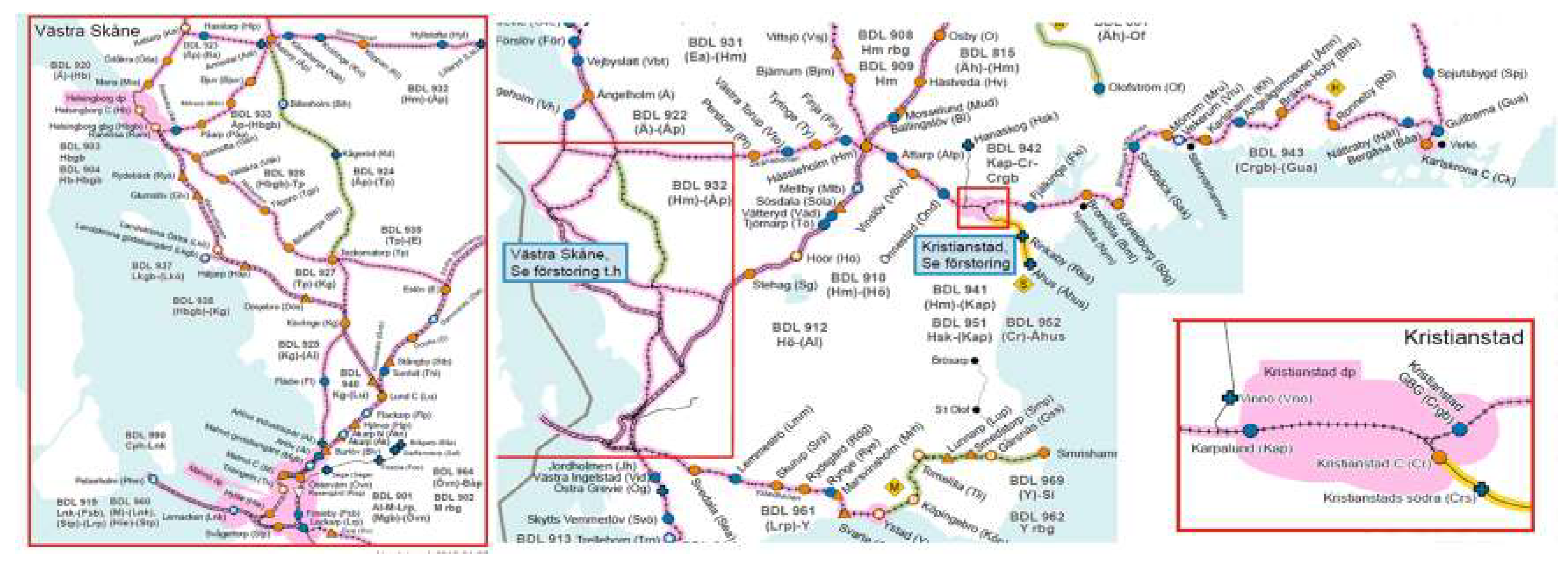
5.1. Experimental Set-Up

For the experimental evaluation, the approach was applied to a number of disturbance scenarios occurring within a selected sub-network in the south of Sweden, namely the railway stretch between Karlskrona city to Malmö, via Kristianstad and Hässleholm (see Figure 4, below). From Karlskrona to Hässleholm, the railway line is single-track, and from Hässleholm to Malmö, the line is double-track with a small portion having four tracks between Arlöv and Malmö. This stretch consists of approximately 90 segments, with a total of 290 block sections. For the regional trains that operate between Karlskrona and Malmö (and even further, into Denmark via the Öresund Bridge), there is a travel time of 1 h and 31 min between Karlskrona and Kristianstad, and a travel time between Kristianstad and Malmö of 1 h and 5 min.

In line with the categorization suggested in [29], three types of disturbance scenarios are used:

• Category 1 refers to a train suffering from a temporary delay at one particular section, which could occur due to, e.g., delayed train staff, or crowding at platforms resulting in increasing dwell times at stations.
• Category 2 refers to a train having a permanent malfunction, resulting in increased running times on all line sections it is planned to occupy.
• Category 3 refers to an infrastructure failure causing, e.g., a speed reduction on a particular section, which results in increased running times for all trains running through that section.

All disturbance scenarios occur between 16:00 and 18:00, which is during peak hours. The re-scheduling time horizons are 1 and 1.5 h time windows, respectively, counting from when the disturbance occurs. The scenarios are described in

Table 3. Description of the 30 × 2 scenarios that were used in the experimental study. The first number in the scenario-ID specifies which disturbance category it is. For category 2, the disturbance is a percentage increase of the runtime, e.g., 40%. The two rightmost columns specify the size of the problem expressed in a number of train events that are to be re-scheduled.

Scenario	Disturbance			Problem Size: #Events 1
Category: ID	Location	Initially Disturbed Train	Initially Delay (min)	1 h Time Window	1.5 h Time Window
1:1	Karlshamn-Ångsågsmossen	1058 (Eastbound)	10	1753	2574
1:2	Bromölla Sölvesborg	1064 (Eastbound)	5	1717	2441
1:3	Kristianstad-Karpalund	1263 (Southbound)	8	1421	2100
1:4	Bergåsa-Gullberna	1097 (Westbound)	10	1739	2482
1:5	Bräkne Hoby-Ronneby	1103 (Westbound)	15	1393	2056
1:6	Flackarp-Hjärup	491 (Southbound)	5	1467	2122
1:7	Eslöv-Dammstorp	533 (Southbound)	10	1759	2578
1:8	Burlöv-Åkarp	544 (Northbound)	7	1748	2572
1:9	Burlöv-Åkarp	1378 (Northbound)	4	1421	2100
1:10	Höör-Stehag	1381 (Southbound)	10	1687	2533
2:1	Karlshamn-Ångsågsmossen	1058 (Eastbound)	40%	1753	2574
2:2	Bromölla Sölvesborg	1064 (Eastbound)	20%	1717	2441
2:3	Kristianstad-Karpalund	1263 (Southbound)	20%	1421	2100
2:4	Bergåsa-Gullberna	1097 (Westbound)	40%	1739	2482
2:5	Bräkne Hoby-Ronneby	1103 (Westbound)	100%	1393	2056
2:6	Flackarp-Hjärup	491 (Southbound)	100%	1467	2122
2:7	Eslöv-Dammstorp	533 (Southbound)	50%	1759	2578
2:8	Burlöv-Åkarp	544 (Northbound)	80%	1748	2572
2:9	Burlöv-Åkarp	1378 (Northbound)	40%	1421	2100
2:10	Höör-Stehag	1381 (Southbound)	40%	1687	2533
3:1	Karlshamn-Ångsågsmossen	All trains passing through	4	1753	2574
3:2	Bromölla Sölvesborg	All trains passing through	2	1717	2441
3:3	Kristianstad-Karpalund	All trains passing through	3	1421	2100
3:4	Bergåsa-Gullberna	All trains passing through	6	1739	2482
3:5	Bräkne Hoby-Ronneby	All trains passing through	5	1393	2056
3:6	Flackarp-Hjärup	All trains passing through	3	1467	2122
3:7	Eslöv-Dammstorp	All trains passing through	4	1759	2578
3:8	Burlöv-Åkarp	All trains passing through	2	1748	2572
3:9	Burlöv-Åkarp	All trains passing through	2	1421	2100
3:10	Höör-Stehag	All trains passing through	2	1687	2533

¹ The size of the generated graph $G$ is the squared size of number of events.

below. The experiments were tested on a laptop with 64-bit Windows 10, equipped with an Intel i7-CPU, 2.60 GHz, with 8 Gigabytes of RAM.

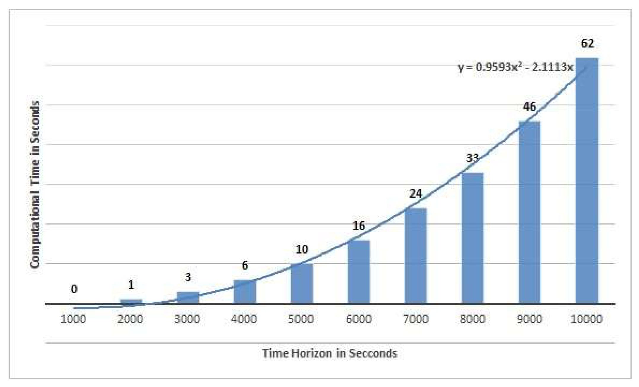
5.2. Results and Analysis

In

Table 4. Computational results for 1 h time horizon.

Scenario	$\mathit{T}\mathit{F}{\mathit{D}}_{\mathit{j}}^{+3}$ Objective Function (hh:mm:ss)							Computational Time (hh:mm:ss)
Category: ID	Optimal Results	Dispatching Rules (DR)						MIP Model	Heuristic Algorithm
		1	2	3	4	5	6
1:1	0:01:03	00:01:14	00:01:14	00:01:14	00:15:22	00:15:22	00:24:05	00:00:04	00:00:06
1:2	0:00:00	00:00:00	00:00:00	00:00:00	00:00:00	00:00:00	01:16:47	00:00:04	00:00:05
1:3	0:00:00	00:02:09	00:02:09	00:02:09	00:36:33	00:36:33	00:26:32	00:00:04	00:00:03
1:4	0:01:02	00:02:28	00:02:28	00:02:28	00:12:40	00:12:40	00:08:11	00:00:06	00:00:06
1:5	0:07:01	00:16:15	00:16:15	00:16:15	00:19:49	00:19:49	00:13:14	00:00:05	00:00:03
1:6	0:00:23	00:05:46	00:05:46	00:05:46	00:05:46	00:05:46	00:05:46	00:00:04	00:00:03
1:7	0:05:05	00:06:24	00:06:24	00:06:24	00:06:24	00:06:24	00:14:45	00:00:04	00:00:05
1:8	0:01:34	00:12:01	00:12:01	00:12:01	00:12:01	00:12:01	00:13:40	00:00:04	00:00:06
1:9	0:00:00	00:14:01	00:14:01	00:14:01	00:13:02	00:13:02	00:14:01	00:00:04	00:00:03
1:10	0:00:00	00:01:18	00:01:18	00:00:00	00:00:00	00:00:00	00:01:33	00:00:04	00:00:05
2:1	0:05:24	00:45:37	00:45:37	00:06:42	00:06:42	00:06:42	00:08:16	00:00:04	00:00:06
2:2	0:02:43	00:03:29	00:39:53	00:03:29	00:03:29	00:03:29	01:06:56	00:00:05	00:00:05
2:3	0:01:01	00:01:47	00:20:06	00:20:06	00:01:47	00:01:47	00:20:14	00:00:03	00:00:03
2:4	0:15:12	00:22:12	00:22:50	00:22:50	00:22:12	00:22:12	00:55:54	00:00:05	00:00:05
2:5	0:42:09	00:43:24	00:58:03	00:58:03	01:05:08	01:05:08	00:59:16	00:00:04	00:00:03
2:6	0:01:24	00:02:44	00:02:44	00:02:44	00:02:44	00:02:44	00:02:44	00:00:06	00:00:04
2:7	0:05:27	00:08:09	00:08:09	00:08:09	00:08:09	00:08:09	00:09:43	00:00:04	00:00:10
2:8	0:21:12	00:43:37	00:38:42	00:38:42	00:43:37	00:43:37	00:40:16	00:00:06	00:00:06
2:9	0:00:00	00:00:00	00:00:00	00:00:00	00:00:00	00:00:00	00:00:00	00:00:05	00:00:03
2:10	0:00:08	00:05:09	00:05:09	00:05:09	00:05:09	00:05:09	00:06:43	00:00:04	00:00:06
3:1	0:01:00	00:01:00	00:01:00	00:01:00	00:01:00	00:01:00	00:25:05	00:00:04	00:00:06
3:2	0:00:00	00:00:00	00:00:00	00:00:00	00:00:19	00:00:19	00:25:54	00:00:04	00:00:06
3:3	0:00:00	00:03:49	00:21:38	01:05:52	00:01:17	00:15:40	00:54:14	00:00:05	00:00:03
3:4	0:12:21	00:16:59	00:20:13	00:20:13	00:16:59	00:16:59	00:20:22	00:00:07	00:00:06
3:5	0:05:20	00:05:25	00:57:34	00:15:58	00:05:25	00:05:25	00:16:12	00:00:03	00:00:03
3:6	0:00:00	00:21:04	00:21:04	00:21:04	00:23:12	00:23:12	00:28:42	00:00:05	00:00:03
3:7	0:00:09	00:07:42	00:14:11	00:14:11	00:14:11	00:14:11	00:15:45	00:00:10	00:00:05
3:8	0:00:00	00:00:00	00:05:06	00:05:06	00:00:00	00:00:00	00:07:54	00:00:04	00:00:05
3:9	0:00:00	00:00:00	00:00:41	00:00:41	00:00:00	00:00:00	00:00:00	00:00:04	00:00:04
3:10	0:00:00	00:04:53	00:04:53	00:03:35	00:01:04	00:01:04	00:02:38	00:00:03	00:00:05

and

Table 5. The computational results for 1.5 h time horizon (hh:mm:ss).

Scenario	$\mathit{T}\mathit{F}{\mathit{D}}_{\mathit{j}}^{+3}$ Objective Function							Computational Time
Category: ID	Optimal Results	Dispatching Rules (DR)						MIP Model	Heuristic Algorithm
		1	2	3	4	5	6
1:1	0:01:03	00:01:14	00:01:14	00:01:14	00:45:13	00:45:13	00:46:56	00:00:12	00:00:20
1:2	0:00:00	00:00:00	00:00:00	00:00:00	00:12:09	00:12:09	05:09:54	00:00:10	00:00:15
1:3	0:00:00	00:02:09	00:02:09	00:02:09	01:34:59	01:34:59	00:25:21	00:00:11	00:00:10
1:4	0:00:00	00:01:27	00:01:27	00:01:27	01:38:16	01:38:16	00:51:24	00:00:13	00:00:16
1:5	0:02:08	00:10:23	00:10:23	00:10:23	00:24:07	00:24:07	00:12:14	00:00:07	00:00:09
1:6	0:00:23	00:05:46	00:05:46	00:05:46	00:05:46	00:05:46	00:05:46	00:00:12	00:00:10
1:7	0:05:05	00:06:24	00:06:24	00:06:24	00:06:24	00:06:24	00:14:45	00:00:11	00:00:18
1:8	0:01:34	00:12:01	00:12:01	00:12:01	00:12:01	00:12:01	00:13:40	00:00:12	00:00:17
1:9	0:00:00	00:13:00	00:13:00	00:13:00	00:13:16	00:13:16	00:38:13	00:00:07	00:00:10
1:10	0:00:00	00:01:18	00:01:18	00:00:00	00:00:00	00:00:00	00:01:33	00:00:11	00:00:16
2:1	0:03:36	00:45:37	00:45:37	00:04:31	00:17:11	00:17:11	00:14:16	00:00:11	00:00:17
2:2	0:00:00	00:00:23	01:21:00	00:00:23	00:00:23	00:00:23	04:36:13	00:00:12	00:00:15
2:3	0:02:40	00:29:31	00:32:58	00:32:58	00:39:25	00:39:25	00:33:46	00:00:07	00:00:09
2:4	0:26:34	00:43:50	01:11:40	01:11:40	00:43:50	00:43:50	01:57:35	00:00:16	00:00:15
2:5	1:11:44	01:17:47	01:40:09	01:40:09	01:41:32	01:41:32	01:35:29	00:00:12	00:00:08
2:6	0:01:24	00:02:44	00:02:44	00:02:44	00:02:44	00:02:44	00:02:44	00:00:11	00:00:09
2:7	0:05:27	00:08:09	00:08:09	00:08:09	00:08:09	00:08:09	00:09:43	00:00:11	00:00:17
2:8	0:21:12	00:44:42	00:48:13	00:48:13	00:44:54	00:44:54	01:08:14	00:00:36	00:00:17
2:9	0:00:00	00:00:00	00:00:00	00:00:00	00:00:13	00:00:13	00:00:00	00:00:07	00:00:10
2:10	0:00:08	00:05:09	00:05:09	00:05:09	00:05:09	00:05:09	00:06:43	00:00:12	00:00:16
3:1	0:00:00	00:00:00	00:22:42	00:00:00	00:00:00	00:00:00	00:46:56	00:00:12	00:00:17
3:2	0:00:00	00:00:17	00:00:17	00:00:17	00:00:36	00:00:36	01:36:46	00:00:11	00:00:14
3:3	0:01:16	00:09:36	00:57:38	01:22:08	00:07:17	00:14:39	02:07:54	00:00:11	00:00:10
3:4	0:16:37	00:31:06	00:32:34	00:32:34	00:23:26	00:23:26	01:10:03	00:00:35	00:00:15
3:5	0:04:44	00:04:58	00:55:43	00:13:08	00:10:16	00:10:16	00:19:59	00:00:10	00:00:09
3:6	0:00:00	00:50:13	00:50:13	00:50:13	00:27:54	00:27:54	01:07:29	00:00:17	00:00:15
3:7	0:00:41	00:06:48	00:15:45	00:15:45	00:15:45	00:15:45	00:17:19	00:00:18	00:00:19
3:8	0:00:00	00:00:00	00:01:22	00:01:22	00:00:00	00:00:00	00:03:58	00:00:11	00:00:17
3:9	0:00:00	00:02:06	00:03:32	00:02:48	00:02:06	00:02:06	00:02:06	00:00:14	00:00:10
3:10	0:00:00	00:08:07	00:08:31	00:07:13	00:01:28	00:01:28	00:03:02	00:00:11	00:00:16

, the results are summarized. The grey cells include the best solution values found by different dispatching rules (DR-1 to DR-6) configurations. These solution values can be compared with the optimal values generated by MIP model. The two rightmost columns compare the computational time for the MIP model and heuristic algorithm. Since the computation time of the algorithm is not significantly affected by the choice of dispatching rule, the computation time is very similar for all six different configurations, and therefore only one computation time value per scenario is presented in Table 4 and Table 5.

The minimum release time goes first (DR-1) was the best dispatching rule, considering the ${\displaystyle \sum }TF{D}_j^{+3}$ objective function. The average ${\displaystyle \sum }TF{D}_j^{+3}$ for the MIP model was 259 s for the 1 h time window and 332 s for the 1.5 h time window. The average ${\displaystyle \sum }TF{D}_j^{+3}$ for the minimum release time goes first (DR-1) was 597 and 849 s, respectively.

Statistical analyses of the results belonging to disturbance scenario type 1 revealed that the less real buffer time goes first (DR-3) dispatching rule, with an average delay of 361 s for a 1 h time window and 314 s for a 1.5 h time window, works better than the other dispatching rules. Additionally, an inefficient solution is not able to absorb the delays (i.e., the delays after a temporary route blocking may remain in the system until midnight). The analysis also shows that for all dispatching rules in scenario 1, the ${\displaystyle \sum }TF{D}_j^{+3}$ objective function values of the 1.5 h time window are lower than the values for the 1 h time window, which confirms that the algorithm successfully attempts to make the timetable absorb delays when possible.

For scenario type 2, the minimum release time goes first (DR-1), less programmed buffer time goes first (DR-4), and less total buffer goes first (DR-5) worked somewhat the same, and better than the others. The average ${\displaystyle \sum }TF{D}_j^{+3}$ objectives were 1056, 953, and 953 s for a 1 h time window, and 1547, 1581, and 1581 for a 1.5 h time window. The optimal values are 568 s for a 1 h time window and 796 s for a 1.5 h time window. In scenario type 3, the minimum release time goes first worked better than the others with an average of 365 s delay, but for a 1.5 h time window the less total buffer goes first (DR-5) with an average of 532 s was the best. The optimal values were 113 and 139 s, respectively.

With the help of a visualization software, the resulting, revised timetables can be analysed beyond aggregated numbers. The more delay goes first (DR-2) dispatching rule gives priority to the trains with the largest tardiness. We observed in the visualization of the solutions that, when the conflict is between two tardy trains, this strategy works well and reduces the delay. However, for conflicts between an on-time train and a tardy train, this dispatching rule gives priority to the tardy train, which causes a delay for an on-time train. In other words, when the tardy train reaches the destination, e.g., Karlskrona or Malmö, this strategy causes a delay for new trains that have recently started the journey. A more effective decision would potentially be to prioritize the on-time train, because the late train is near to its final destination.

The less real buffer time goes first (DR-3) dispatching rule, gives priority to the train with least buffer time. This strategy helps the algorithm to reduce the delay for tardy trains. When the conflict is between two tardy trains, this policy is fair. The less programmed buffer time goes first (DR-5) considers the sum of buffer time for a train to its destination. In a disturbance area, this strategy works well. The algorithm gives priority to a train with less programmed buffer time, which seems to be fair between two tardy trains. However, when a tardy train has a conflict with an on-time train, this dispatching rule gives priority to the tardy one, which is not effective if the on-time train is at the beginning of its itinerary and thus may cause knock-on delays if it is delayed. The less total processing time (DR-6) dispatching rule, tries to give priority to trains with less remaining events to leave the tracks as soon as possible. The experimental results demonstrate that this strategy does not work well compared to other dispatching rules.

The choice of dispatching rule does not affect the computational time, but the number of events in the re-scheduling time window and selected sub-network has a significant effect on the computational time since the size of the graph $G$ increases quadratically. Figure 5 illustrates the increase of computational time against increase of the time horizon and number of events. Both the size of graph $G$ and the computational time increase quadratically.

6. Conclusions and Future Work

This paper addresses the real-time train traffic re-scheduling problem. A mixed graph is used for modeling the problem as a blocking job-shop scheduling problem. A heuristic algorithm is proposed that benefits from re-timing, re-ordering, and local re-routing. The algorithm benefits also from a dynamic update of data, which accelerates the computations.

The response time for such a real-time computational scheduling tool is a vital factor. In the proposed solution approach, the problem for a 1 h time window is solved in less than 10 s, and for a 1.5 h time window, the computational time is less than 20 s. It is also unknown what time horizon is necessary to consider in different situations and what role this uncertainty would play. Interviews with dispatchers suggest that it differs a lot depending on the situation, context and associated working load.

The $TF{D}_j^{+3}$ objective function is a relevant criterion to control the lateness of trains. However, based on the situation and type of disturbance scenario, the dispatchers also have other concerns and objectives. The investigation of other objective functions and useful solution quality metrics is necessary to investigate in future research. The graph $G$ is represented by an adjacency matrix in the current implementation. Using alternative data structures such as adjacency lists, can be an option to investigate the possibility to reduce computational time further.

References

1. Boston Consultancy Group. The 2017 European Railway Performance Index; Boston Consultancy Group: Boston, MA, USA, 18 April 2017. [Google Scholar]
2. European Commission Directorate General for Mobility and Transport. Study on the Prices and Quality of Rail Passenger Services; Report Reference: MOVE/B2/2015-126; European Commission Directorate General for Mobility and Transport: Brussel, Belgium, April 2016. [Google Scholar]
3. Lamorgese, L.; Mannino, C.; Pacciarelli, D.; Törnquist Krasemann, J. Train Dispatching. In Handbook of Optimization in the Railway Industry, International Series in Operations Research & Management Science; Borndörfer, R., Klug, T., Lamorgese, L., Mannino, C., Reuther, M., Schlechte, T., Eds.; Springer: Cham, Switzerland, 2018; Volume 268. [Google Scholar] [CrossRef]
4. Cacchiani, V.; Huisman, D.; Kidd, M.; Kroon, L.; Toth, P.; Veelenturf, L.; Wagenaar, J. An overview of recovery models and algorithms for real-time railway rescheduling. Transp. Res. B Methodol. 2010, 63, 15–37. [Google Scholar] [CrossRef]
5. Fang, W.; Yang, S.; Yao, X. A Survey on Problem Models and Solution Approaches to Rescheduling in Railway Networks. IEEE Trans. Intell. Trans. Syst. 2015, 16, 2997–3016. [Google Scholar] [CrossRef]
6. Josyula, S.; Törnquist Krasemann, J. Passenger-oriented Railway Traffic Re-scheduling: A Review of Alternative Strategies utilizing Passenger Flow Data. In Proceedings of the 7th International Conference on Railway Operations Modelling and Analysis, Lille, France, 4–7 April 2017. [Google Scholar]
7. Szpigel, B. Optimal train scheduling on a single track railway. Oper. Res. 1973, 72, 343–352. [Google Scholar]
8. D’Ariano, A.; Pacciarelli, D.; Pranzo, M. A branch and bound algorithm for scheduling trains in a railway network. Eur. J. Oper. Res. 2017, 183, 643–657. [Google Scholar] [CrossRef]
9. Khosravi, B.; Bennell, J.A.; Potts, C.N. Train Scheduling and Rescheduling in the UK with a Modified Shifting Bottleneck Procedure. In Proceedings of the 12th Workshop on Algorithmic Approaches for Transportation Modelling, Optimization, and Systems 2012, Ljubljana, Slovenia, 13 September 2012; pp. 120–131. [Google Scholar]
10. Liu, S.; Kozan, E. Scheduling trains as a blocking parallel-machine job shop scheduling problem. Comput. Oper. Res. 2009, 36, 2840–2852. [Google Scholar] [CrossRef] [Green Version]
11. Mascis, A.; Pacciarelli, D. Job-shop scheduling with blocking and no-wait constraints. Eur. J. Oper. Res. 2002, 143, 498–517. [Google Scholar] [CrossRef]
12. Oliveira, E.; Smith, B.M. A Job-Shop Scheduling Model for the Single-Track Railway Scheduling Problem; Research Report Series 21; School of Computing, University of Leeds: Leeds, UK, 2000. [Google Scholar]
13. Törnquist, J.; Persson, J.A. N-tracked railway traffic re-scheduling during disturbances. Transp. Res. Part B Methodol. 2007, 41, 342–362. [Google Scholar] [CrossRef]
14. Pellegrini, P.; Douchet, G.; Marliere, G.; Rodriguez, J. Real-time train routing and scheduling through mixed integer linear programming: Heuristic approach. In Proceedings of the 2013 International Conference on Industrial Engineering and Systems Management (IESM), Rabat, Morocco, 28–30 October 2013. [Google Scholar]
15. Xu, Y.; Jia, B.; Ghiasib, A.; Li, X. Train routing and timetabling problem for heterogeneous train traffic with switchable scheduling rules. Transp. Res. Part C Emerg. Technol. 2017, 84, 196–218. [Google Scholar] [CrossRef]
16. Corman, F.; D’Ariano, A.; Pacciarelli, D.; Pranzo, M. Centralized versus distributed systems to reschedule trains in two dispatching areas. Public Trans. Plan. Oper. 2010, 2, 219–247. [Google Scholar] [CrossRef]
17. Corman, F.; D’Ariano, A.; Pacciarelli, D.; Pranzo, M. Optimal inter-area coordination of train rescheduling decisions. Trans. Res. Part E 2012, 48, 71–88. [Google Scholar]
18. Corman, F.; Pacciarelli, D.; D’Ariano, A.; Samá, M. Rescheduling Railway Traffic Taking into Account Minimization of Passengers’ Discomfort. In Proceedings of the International Conference on Computational Logistics, ICCL 2015, Delft, The Netherlands, 23–25 September 2015; pp. 602–616. [Google Scholar]
19. Lamorgese, L.; Mannino, C. An Exact Decomposition Approach for the Real-Time Train Dispatching Problem. Oper. Res. 2015, 63, 48–64. [Google Scholar] [CrossRef]
20. Meng, L.; Zhou, X. Simultaneous train rerouting and rescheduling on an N-track network: A model reformulation with network-based cumulative flow variables. Trans. Res. Part B Methodol. 2014, 67, 208–234. [Google Scholar] [CrossRef]
21. Tormo, J.; Panou, K.; Tzierpoulos, P. Evaluation and Comparative Analysis of Railway Perturbation Management Methods. In Proceedings of the Conférence Mondiale sur la Recherche Dans les Transports (13th WCTR), Rio de Janeiro, Brazil, 15–18 July 2013. [Google Scholar]
22. Rodriguez, J. An incremental decision algorithm for railway traffic optimisation in a complex station. Eleventh. In Proceedings of the International Conference on Computer System Design and Operation in the Railway and Other Transit Systems (COMPRAIL08), Toledo, Spain, 15–17 September 2008; pp. 495–504. [Google Scholar]
23. Bettinelli, A.; Santini, A.; Vigo, D. A real-time conflict solution algorithm for the train rescheduling problem. Trans. Res. Part B Methodol. 2017, 106, 237–265. [Google Scholar] [CrossRef]
24. Samà, M.; D’Ariano, A.; Corman, F.; Pacciarelli, D. A variable neighbourhood search for fast train scheduling and routing during disturbed railway traffic situations. Comput. Oper. Res. 2017, 78, 480–499. [Google Scholar] [CrossRef]
25. Burdett, R.L.; Kozan, E. A sequencing approach for creating new train timetables. OR Spectr. 2010, 32, 163–193. [Google Scholar] [CrossRef] [Green Version]
26. Tan, Y.; Jiang, Z. A Branch and Bound Algorithm and Iterative Reordering Strategies for Inserting Additional Trains in Real Time: A Case Study in Germany. Math. Probl. Eng. 2015, 2015, 289072. [Google Scholar] [CrossRef]
27. Gholami, O.; Sotskov, Y.N. A fast heuristic algorithm for solving parallel-machine job-shop scheduling problems. Int. J. Adv. Manuf. Technol. 2014, 70, 531–546. [Google Scholar] [CrossRef]
28. Sotskov, Y.; Gholami, O. Mixed graph model and algorithms for parallel-machine job-shop scheduling problems. Int. J. Prod. Res. 2017, 55, 1549–1564. [Google Scholar] [CrossRef]
29. Krasemann, J.T. Design of an effective algorithm for fast response to the re-scheduling of railway traffic during disturbances. Transp. Res. Part C Emerg. Technol. 2012, 20, 62–78. [Google Scholar] [CrossRef]
Figure 1. Presenting a conflict in a graph G : (a) using an edge in the mixed graph model to present a conflict between the two operations; (b) using two arcs in the alternative graph model to present a conflict between two operations.
Algorithms 11 00055 g001
Figure 2. Resolving the conflicts on the machine m 1 and m 2 in a graph G : (a) conflict resolution using the mixed graph model; (b) conflict resolution using the alternative graph model to support the blocking condition.
Algorithms 11 00055 g002
Figure 3. Adding the clear time and headway time distance to the alternative graph: (a) the starting time of operation o 2 , 1 is increased due to the clear time; (b) the starting time of operation o 2 , 1 is increased due to the headway distance.
Algorithms 11 00055 g003
Figure 4. Illustration of the studied railway line Karlskrona-Kristianstad-Malmö. Source: Trafikverket.
Algorithms 11 00055 g004
Figure 5. The computational time increases quadratically, based on the number of events.
Algorithms 11 00055 g005