Hadoop vs. Spark: Impact on Performance of the Hammer Query Engine for Open Data Corpora

Abstract

The Hammer prototype is a query engine for corpora of Open Data that provides users with the concept of blind querying. Since data sets published on Open Data portals are heterogeneous, users wishing to find out interesting data sets are blind: queries cannot be fully specified, as in the case of databases. Consequently, the query engine is responsible for rewriting and adapting the blind query to the actual data sets, by exploiting lexical and semantic similarity. The effectiveness of this approach was discussed in our previous works. In this paper, we report our experience in developing the query engine. In fact, in the very first version of the prototype, we realized that the implementation of the retrieval technique was too slow, even though corpora contained only a few thousands of data sets. We decided to adopt the Map-Reduce paradigm, in order to parallelize the query engine and improve performances. We passed through several versions of the query engine, either based on the Hadoop framework or on the Spark framework. Hadoop and Spark are two very popular frameworks for writing and executing parallel algorithms based on the Map-Reduce paradigm. In this paper, we present our study about the impact of adopting the Map-Reduce approach and its two most famous frameworks to parallelize the Hammer query engine; we discuss various implementations of the query engine, either obtained without significantly rewriting the algorithm or obtained by completely rewriting the algorithm by exploiting high level abstractions provided by Spark. The experimental campaign we performed shows the benefits provided by each studied solution, with the perspective of moving toward Big Data in the future. The lessons we learned are collected and synthesized into behavioral guidelines for developers approaching the problem of parallelizing algorithms by means of Map-Reduce frameworks.

1. Introduction

Open Data portals have become tools widely adopted by public administrations to diffuse data sets concerning territories and governments; since these data sets are publicly available to anybody, they are called “open”.

In [1], we started a research project whose aim is to develop a technique for blind querying corpora of Open Data. The idea of blind querying is motivated by the fact that a corpus of Open Data possibly contains thousands of data sets, each one with its own structure that is unknown to users wishing to look for interesting data sets.

The retrieval technique introduced in [1] has been further extended and improved in [2]; in both papers, we discussed the effectiveness of the technique in terms of recall and precision. In particular, we compared our technique with Apache Solr; it is based on Apache Lucene like ElasticSearch: both are feature-rich search engines and more or less give the same performance; however, Apache Solr is recommended for text-oriented search engines and Elasticsearch is better to handle analytical queries. Apart from better recall and precision we obtained with our technique, the main difference is that our technique does not have to index (possibly huge) instances of data sets, but only meta-data: instances are downloaded only in the final phase of retrieval, at query time. In practice, our technique can query several Open Data portals from an external server. Neither Apache Solr nor ElasticSearch can do this.

The retrieval technique that enables blind querying was implemented in the Hammer prototype, in order to test it and prove its feasibility. However, the very first version of the implementation was too slow, even with a few thousands of indexed data sets. Consequently, we decided to adopt the Map-Reduce paradigm and its most popular frameworks, i.e., Hadoop and Spark, to find out how to improve performances.

The Map-Reduce paradigm is a technique to simplify the development of parallel algorithms in the context of Big Data analysis. The idea is that the programmer has to think of tasks to perform, focusing on the problem to solve; it will be responsibility of the execution framework to control computation in a totally transparent way.

However, the availability of different frameworks and, for the same framework, different abstractions for implementing Map-Reduce strategy, makes it difficult for developers to approach the adoption of this paradigm.

In this paper, we report our experience in adopting the Map-Reduce paradigm within the Hammer query engine. We describe the native algorithms and how we transformed it to make it parallel and more efficient. The first step was to make the minimal changes necessary to parallelize computation, maintaining the original structure of the algorithm. We first realized the parallel version on top of the Hadoop framework. Then, we adopted the Spark framework. These two implementations gave us the possibility to understand the different behavior exhibited by the two frameworks. Then, to further improve performances, we redesigned completely the algorithm, to exploit the high-level abstraction provided by Spark called ”dataset”: this abstraction allows developers to think differently about the algorithm, simplifying procedures and fastening the development process; furthermore, high-level operations on datasets are automatically executed in Map-Reduce mode when necessary, in a totally transparent way.

In this paper, we report our experience concerning the adoption of the Map-Reduce paradigm and its frameworks. In particular, the experimental campaign we performed shows the benefits provided by each studied solution, with the perspective of moving toward Big Data in the future. The lessons we learned are collected and synthesized into behavioral guidelines for developers approaching the problem of parallelizing algorithms by means of Map-Reduce frameworks.

As far as our previous work is concerned, the contributions of this paper are manifold. First of all, a necessary premise gives an overview of the concept of blind querying of Open Data corpora, briefly reporting the retrieval technique. Then, a short overview of the Map-Reduce paradigm and of main features of Hadoop and Spark is given as well. After that, the paper provides the following contributions:

• a detailed description of the architecture of the prototype, which will help us in analyzing performance;
• the algorithm that implements the critical step of our blind querying technique (Step 4, see Section 3.3) is precisely described; its variants necessary to adapt it to Hadoop and Spark are also presented;
• an extensive study about performance of Hadoop and Spark implementations is reported;
• a critical analysis of performance is done, in order to compare the compared solutions;
• we report the lessons we learned by the analysis of execution times, and we give some behavioral guidelines for developers wishing to transform non algorithms into Map-Reduce algorithms.

The paper is organized as follows: Section 2 discusses relevant related works. Section 3 introduces the general framework for blind querying Open Data corpora, where the retrieval technique is summarized. Section 4 presents the Map-Reduce paradigm and the main features of Hadoop and Spark. Section 5 presents the Hammer prototype: Section 5.1 introduces the architecture; Section 5.2 presents the basic non-parallel algorithm; Section 5.3 presents the first Map-Reduce evolution of the algorithm, while Section 5.4 presents the enhanced version based on high-level abstractions provided by Spark. Section 6 reports the extensive experimental campaign we performed, by discussing results. Section 7 reports the lessons we learned and the behavioral guidelines for developers. Section 8 draws conclusions and future work.

2. Related Works

We started our research on blind querying of Open Data corpora with [1]; the technique has been subsequently enhanced in [2]; this latter paper is the basis for the implementation of the Hammer prototype discussed in this paper. We previously discussed how to use Map-Reduce in the various components of the Hammer prototype in [3]; however, a deep analysis of performance was not performed. After these works, we think we are still the pioneers on this research line: it seems that no strictly related works are in literature. For this reason, it is not possible to perform a direct comparison with other approaches. Consequently, we will discuss more in general the world of Open Data and the world of Map-Reduce computation.

The world of Open Data is becoming more and more important for many human activities. Due to the wider and wider diffusion of Open Data portals, Open Data Management research is becoming more and more important, although this area is just at the beginning of its development. We can say that our vision of the problem was inspired by [4], where the authors observe characteristics of fifty Open Data repositories.

In [5], the authors note that there is a growing number of applications that require access to both structured and unstructured data. Such collections of data have been referred to as dataspaces, and Dataspace Support Platforms (DSSP) were proposed to offer several services over dataspaces. One of the key services of a DSSP is seamless querying on the data. The Hammer prototype can be seen as DSSP of Open Data, while Reference [5] proposes a DSSP of web pages.

In [6], the authors describe their approach and their idea to build a pool of federated Open Data corpora with SPARQL as query language. However, we considered SPARQL only for people that are highly skilled in computer science: our query technique is very easy to use and it is designed for analysts with medium-level or low-level skills in computer science.

We now consider the area concerned with Map-Reduce. Reference [7] introduced the Map-Reduce paradigm. In fact, with the upcoming advent of the concept of Big Data, it was clear that parallel computation had to be the straightforward solution to deal with very large data sets. However, it was also clear that traditional approaches to write parallel programs were not suitable, because they require the high expertise to design such programs. Map-Reduce is Columbus’ Egg: the hard part of parallel computing is automatically dealt with by the execution layer.

After some early prototype systems, Hadoop was developed and has become very popular [8,9]. Certainly, the choice of implementing as a Java library has helped its diffusion; nevertheless, it was effective in solving compuational problems in hard contexts. The fact that Facebook decided to adopt it [10] is the best proof in this respect.

However, Hadoop has exhibited an important issue concerned with execution times, in particular for iterative algorithms: the HDFS (Hadoop Distributed File System) is slow as far as sharing of data blocks among tasks is concerned. Consequently, Spark [11] was developed to solve this problem. The solution is the adoption of a main-memory abstraction called Resilient Distributed Dataset (RDD), which replaces HDFS for sharing data blocks. The effects are impressive: various studies [12] demonstrated that in most situations Spark dramatically overcomes Hadoop, provided that the cluster is equipped with enough main memory.

Looking at applications, they are so many that it is practically impossible to list them all. We only provide the reader with some hints. One topic where Map-Reduce is being investigated and/or adopted is machine learning. Refs. [13,14,15] reports experiences made to implement various machine learning techniques based on Map-Reduce; in particular, Reference [16] is an example of adopting Spark.

The field of data mining has been investigated too, in order to apply Map-Reduce; Reference [17] shows how many techniques can be implemented by exploiting Map-Reduce. Within this field, the topic of mining association rules has been investigated too: Refs. [18,19] are just a few of the papers on the topic.

Finally, the field of data management has been touched as well by Map-Reduce diffusion. One important topic is the distributed execution of queries over relational databases [20], but NoSQL databases have been considered as well [21].

Data storage systems that provide information retrieval capabilities have become popular in recent years. For example, ElasticSearch [22] is now widely used, even in industrial contexts. Another interesting system is Apach Solr [23], which can be considered a kind of more academic version of ElasticSearch. More or less, they provide similar capabilities, since they are both based on Apache Lucene. Compared with our approach. they need to fully load data set instances to index their content, while our Hammer prototype indexes only meta-data; furthermore, they do not provide structured queries with object selection condition, as our query language does.

3. A Framework for Blind Querying

In this section, we present the framework for blind querying a corpus of data sets.

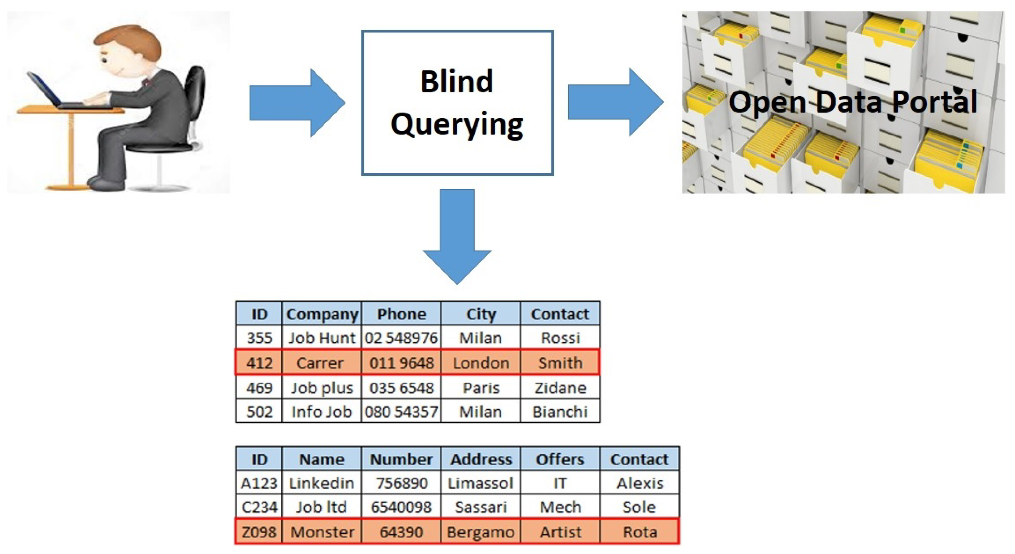
3.1. Concepts, Definitions and Problem

Definition 1.

Data Set. A Data Set $ds$ is a set of homogeneous objects (i.e., having the same schema). It is described by a tuple (data set descriptor)

$$ds:<ds\_id dataset\_name, schema, metadata>,$$

where $ds\_id$ is a unique identifier, $dataset\_name$ is the name of the data set (not unique); $schema$ is a set of field names contained in objects belonging to the data set; $metadata$ is a set of pairs(label, value), which are additional meta-data associated with the data set.

The instance of the data set is the actual set of objects in the data set.

In our model, a data set instance contains objects, specifically, JSON (JavaScript Object Notation) objects. In fact, the traditional format for open data sets is as CSV (comma-separated values) files, where each data item is a row; the first row of the file reports the schema (list of field names) of the data set; consequently, the other rows have the same structure. A CSV file can be easily represented as an array of flat JSON objects, all having the same flat structure.

Nevertheless, JSON has become a very popular format for data exchange; many data sets on Open Data portals are provided as JSON data sets. In this case, a data set is an array of JSON objects. They usually are the straightforward representation of flat CSV files; however, even if they are not, objects in the data sets all have the same structure. This is why we decided to rely on the concept of (JSON) object to deal with data items.

Definition 2.

Corpus and Catalog. With C = {$d{s}_1$, $d{s}_2$, …} , we refer the corpus of data sets. The catalog of the corpus is the list of descriptors, i.e., meta-data, of data sets in C (see Definition 1).

We can now specify the concept of Query, in order to illustrate our approach for blind querying a corpus of data sets.

Definition 3.

Query. Given a Data Set Name $dn$, a set P of field names (properties) of interest $P=\{p{n}_1,p{n}_2,\dots \}$ and a selection condition $sc$ on field values, a query q is a triple $q:<dn,P,sc>$ (This definition appeared in [2]).

In order to introduce the general idea behind blind querying and to clarify the query technique in the remainder of the paper, we need to introduce the concept of query term.

Definition 4.

Query Term. Consider a query $q:<dn,P,sc>$. With Query Term (term for simplicity), we denote a data set name $q.dn$, a field name appearing in $q.P$ or in $q.sc$, a constant appearing in $q.sc$ (This definition appeared in [2]).

A term could be composed of many words, separated by blank spaces, underscores or lines. In fact, in JSON, field names can contain blanks, underscores and lines.

Example 1.

Figure 1 depicts the application scenario. The user wishing to find interesting data sets on an Open Data portal can perform a blind query without knowing anything about the data sets published by the portal. It is the responsibility of the query engine to address the query to the portal, possibly rewriting the query in order to capture lexically or semantically similar terms actually present in the catalog of the corpus. The result is a pool of data sets possibly meeting the wishes of the user.

As a concrete example, suppose a labour-market analyst wants to get information about job offers for “Data Scientist” located in a given city named “My City”. The query could be

$q:<$dn = [Job-Offers],

   P $=\{$ [Company], [Skills], [Contract]},

    sc $=($ [Location]="My City" AND

        [Profession]="Data Scientist"$)>$.

However, in the Open Data portal, there could not exist a data set with name Job-Offers: desired job vacancies could be in a different data set named Jobs. Thus, objects of interest could be retrieved by a slightly different query, i.e.,

$n{q}_1:<$dn=[Jobs],

   P $=\{$ [Company], [Skills], [Contract]},

   sc $=($[Location]="My City" AND

        [Profession]="Data Scientist"$)>$.

Query $n{q}_1$ is obtained by rewriting query q: the data set name $q.dn=$ [Job-Offers] is substituted with Jobs. In the rewritten query, it becomes $n{q}_1.dn=$ [Jobs].

Another possible rewritten query could be obtained by changing property City with Job-Location. In this case, we obtain the following rewritten query $n{q}_2$:

$n{q}_2:<$dn=[Job-Offers],

   P $=\{$ [Company], [Skills], [Contract]},

   sc $=($[Job-Location]="My City" AND

        [Profession]="Data Scientist"$)>$.

The substitution of a term with a similar one originates a new query that could find out data sets containing objects of interest for the analysts.

Furthermore, another rewritten query $n{q}_3$ could be obtained by substituting two terms:

$n{q}_3:<$dn=[Jobs],

   P $=\{$ [Company], [Skills], [Contract]},

   sc $=($[Job-Location]="My City" AND

        [Profession]="Data Scientist"$)>$.

Query $n{q}_3$ looks for a data set named Jobs and selects objects with the field Job-Location having a value "My City".

Queries $n{q}_1$, $n{q}_2$ and $n{q}_3$, similar to the original one q, constitute the neighborhood of q; for this reason, they are called Neighbour Queries.

The concept of Neighbour Queries is the key of the technique: the search space is expanded, by exploiting information in the catalog of the corpus, on the basis of lexical similarity as well as semantic similarity of query terms.

Problem 1.

Given a corpus C of data sets and a query q, return the result set $RS=\{o_1,o_2,\dots \}$, which contains objects $o_i$ retrieved in data sets $d{s}_j\in C$ ($o_i\in Instance(d{s}_j$)) such that $o_i$ satisfies query q or a neighbour query $nq$ that is obtained by rewriting query q.

The Hammer prototype implements our technique to solve the problem. In the remainder of the section, we summarize pre-processing steps and the retrieval technique.

3.2. Pre-Processing

In Section 3.3, we present the general retrieval technique based on the concept of blind querying, which we implemented within the Hammer prototype. However, before querying is possible, some pre-processing activities are necessary.

• Scanning the Portal. The portal, containing data sets to add to the corpus C, is scanned, in order to get the complete list of available data sets.
• Retrieving Meta-data of data sets. From the portal, for each data set, its meta-data and schema are retrieved.
• Building the Catalog. The catalog of the corpus is built, in order to collect meta-data and schemas of data sets.
• Indexing. An inverted index [24] is built, on the basis of meta-data and schemas of data sets.

At the end of pre-processing, the corpus C has its catalog and is indexed. The inverted index will be exploited at query time, as described in Section 3.3.

3.3. Retrieval Technique

The technique we developed for blind querying is fully explained in [2]. Here, we report a synthetic description (from [2]), with the goal to let the reader understand the rest of the paper.

The proposed technique is built around a query mechanism based on the Vector Space Model (VSM) [25], encompassed in a multi-step process devised to deal with the blind querying approach based on a query rewriting technique.

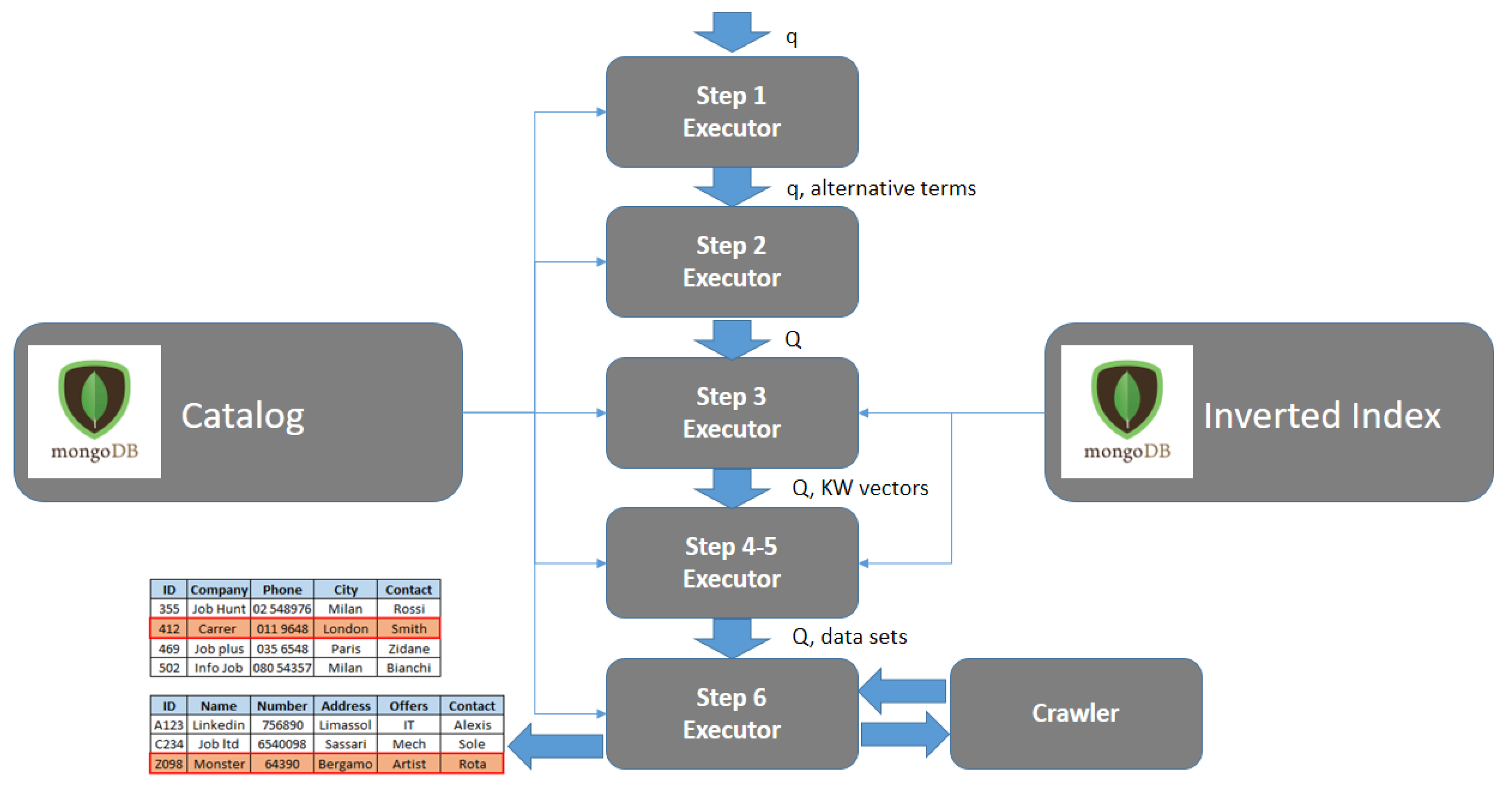
• Step 1: Term Extraction and Retrieval of Alternative Terms. The set $T\left(q\right)$ of terms is extracted from within the query q. Then, for each term $t\in T\left(q\right)$, the set $Alt\left(t\right)$ of similar terms is built. A term $t^{\prime }\in Alt\left(t\right)$ either if it is lexicographically similar (based on the Jaro-Winkler similarity measure [26]) or semantically similar (synonym) based on WordNet dictionary, or a combination of both. Terms in $Alt\left(t\right)$ are actually present in the catalog of the corpus.
• Step 2: Generation of Neighbour Queries. For each term $t\in T\left(q\right)$, alternative terms $Alt\left(t\right)$ are used to derive, from the original query q, the Neighbour Queries $nq$, i.e., queries which are similar to q. Both q and the derived neighbour queries are in the set Q of queries to process.
• Step 3: Keyword Selection. For each query to process $nq\in Q$, keywords $K\left(nq\right)$ are selected from terms in $nq$, in order to find the most representative/informative terms for finding potentially relevant data sets (introduced and extensively described in [1]).
  For each query $nq\in Q$, its keyword vector K(nq) is computed: it is represented as a vector K(nq) = [$k_1$, …, $k_n$]; the accompanying vector $\overline{w}$(nq) = [${\overline{w}}_1$, …, ${\overline{w}}_n$] represents the weight ${\overline{w}}_i$ of each term $k_i$ in vector K(nq); each weight ${\overline{w}}_i\in [0,1]$ is the result of the previous steps, on the basis of (lexical or semantic) similarity with respect to original terms (see [2]).
• Step 4: VSM Data Set Retrieval. For each query $nq\in Q$, the selected keywords $K\left(nq\right)$ are used to retrieve data sets based on the Vector Space Model [25] approach: in this way, the set of possibly relevant data sets is obtained. Notice that we select only data sets with a similarity measure krm $\in [0,1]$ (cosine similarity with respect to a query $nq\in Q$) greater than or equal to a minimum threshold th_krm.
  Specifically, given a data set $d{s}_i$, vector

  $$W\left(d{s}_i\right)=[w_1,\dots ,w_n]$$

  is the vector of weights of each keyword $k_h$ for data set $d{s}_i$, obtained through the inverted index (refer to [2] for details).
  The Keyword-based Relevance Measure $krm(d{s}_i,n{q}_J)\in [0,1]$ for data set $d{s}_i$ with respect to query $nq$ is the cosine of the angle between vectors $\overline{w}\left(nq\right)$ and W($d{s}_i$).
  When $krm(d{s}_i,n{q}_J)=1$, the data set is associated with all the keywords of the original query.
• Step 5: Schema Fitting. The full set of field names in each query $nq\in Q$ is compared with the schema of each selected data set, in order to compute the Schema Fitting Degree $sfd(d{s}_i,nq)\in [0,1]$. Data sets whose schema better fits the query will be more relevant than other data sets. For this reason (refer to [2]), the relevance measure of a data set $rm\left(d{s}_i\right)$ is defined as a weighted composition of keyword relevance measure $krm$ and schema fitting degree $sfd$. A minimum threshold th_rm is set, to select relevant data sets.
• Step 6: Instance Filtering. Instances of relevant data sets are processed (i.e., downloaded from the portal and filtered) in order to filter out and keep only the objects that satisfy the selection condition. The result set is so far built: it is a collection of JSON objects.

To run the query process, three minimum thresholds must be set: the first one is the minimum string similarity threshold th_sim $\in [0,1]$, used to select lexicographically similar terms; the second one is the minimum keyword relevance threshold th_krm $\in [0,1]$ for cosine similarity of data sets with respect to queries in Q; the third one is the minimum relevance threshold th_rm $\in [0,1]$ for data sets.

4. Map-Reduce: Approach and Frameworks

In this section, we first introduce the main concepts concerning Map-Reduce programming; then, we briefly present the two most famous Map-Reduce frameworks, i.e., Hadoop and Spark.

4.1. The Map-Reduce Approach

The Map-Reduce programming paradigm was introduced in [7]. The goal of the authors was to separate the definition of the (possibly simple) computation from the (possibly complex) problem of parallelizing the execution. In fact, the authors argued that most of problems concerned with data transformation are conceptually simple problems; however, their simplicity disappears when they must be parallelized, in order to get an answer in a reasonable time when very large data sets (such as the case of Big Data) are processed. The idea is to define a programming abstraction based on two functional primitives, by means of which to express the transformation. It will be responsibility of the execution layer to handle hard issues of parallel execution.

Let us give a short description of the approach. Two primitives are available for programmers to write procedures: Map and Reduce.

• Map primitive: this primitive is a programmer-defined function that processes (usually) small parts of input data in order to generate a set of intermediate key/value pairs. Keys will play the role of grouping values in the next Reduce step.
• Reduce primitive: this primitive is a programmer-defined function that takes the set of key/value pairs generated in the Map phase and aggregate pairs with the same key.

Programmers have only to define the two functions, i.e., how to generate key/value pairs and what aggregation to compute from a set of aggregated pairs. It is the responsibility of the underlying execution layer to perform the following activities:

• distributing data to computing nodes;
• collecting key/value pairs;
• distributing key/value pairs to nodes, in order to aggregate them.

As an example, consider the generation of the inverted index. Given a data set $ds$ and the set of terms appearing in its schema and meta-data, the Map phase builds pairs $(term,ds\_id)$; the Reduce phase aggregates all pairs into the inverted index, in such a way a term is associated with the list of identifiers of data sets that contain that term (in fact, we implemented the indexing phase by means of Map-Reduce as well [3], but its description is outside the scope of the paper).

Iterative Algorithms

The Map-Reduce paradigm is particularly suitable for expressing simple transformations that can be depicted as a non-cyclic graph. An example could be building an inverted index (as previously discussed): only one Map-Reduce flow is necessary.

However, many transformations and computations are necessarily iterative processes, where each iteration relies on outputs produced by the previous iteration. Such algorithms can be described by means of the Map-Reduce paradigm as well: each iteration is a single Map-Reduce flow; the overall computation consists of as many Map-Reduce flows as the number of iterations.

4.2. Hadoop vs. Spark

Currently, the two most-popular open-source frameworks for executing Map-Reduce processes are Hadoop and Spark.

Hadoop is the first popular Map-Reduce framework. The reader can refer to [27] as a complete guide, to understand technicalities of the framework. Here, we summarize its main features. It has been designed to be a general framework suitable for various types of Big Data applications, possibly based on iterative algorithms. Two layers compose Hadoop:

• a data storage layer called Hadoop Distributed File System (HDFS) [28], which provides storage support to process, both for input data and for intermediate results;
• a data processing layer called Hadoop Map-Reduce Framework, which distributes and coordinates computation on the cluster; the basic component, which actually handles task execution, is named YARN (Yet Another Resource Negotiator) [29].

Data in HDFS are organized in blocks; single blocks are distributed to Map tasks (for each block, a processing task is created), as well as they are dispatched to one or many Reduce tasks. Iterative algorithms perform multiple Hadoop Map-Reduce flows; data are shared through HDFS: input data of each iteration are read from HDFS, as well as output data must be written back to HDFS, for each iteration. Consequently, the large amount of disk accesses and data exchanges through the network cause a significant overhead that is paid in terms of execution times. In this respect, many works, such as [9,30,31], studied the behavior of iterative algorithms within Hadoop.

Spark [11] is a more recent Map-Reduce framework than Hadoop. It has been designed [32] to overcome the issue exhibited by Hadoop in terms of high execution times, in particular for iterative algorithms, caused by the fact that the only way to share data is through the distributed file system HDFS.

The abstraction provided by Spark to overcome this issue is the concept of Resilient Distributed Dataset (RDD). It is a block of data that is shared to processing tasks through the main memory of computational devices in the cluster. Computational flows are performed as described hereafter.

• Input data are transferred from persistent memory to main memory, subdivided in many RDDs; these RDDs are read-only for next tasks.
• Computational tasks are performed by worker nodes; they access RDDs and generate new RDDs;
• A RDD is resilient because the framework keeps track of the process that has generated it. In case of loss of its content (due to space limitations in main memory), the framework rebuilds the RDD, by re-executing the tasks that have generated the lost RDD.

This way, Spark is expected to be much more efficient than Hadoop, in particular for iterative algorithms, provided that the main memory actually available on the cluster is sufficient to store all RDDs. The reader can refer to [12] for a comparative analysis of performance with Hadoop, where a Page Rank algorithm is used as a testbed.

5. The Hammer Prototype

We now illustrate the Hammer prototype. First of all, we present its architecture in Section 5.1. In Section 5.2, we present the basic algorithm we implemented for Step 4 and Step 5. Then, in Section 5.3, we show how this basic algorithm was easily converted into a Map-Reduce algorithm. In Section 5.4, we show how we redesigned the algorithm by exploiting high-level abstractions provided by Spark.

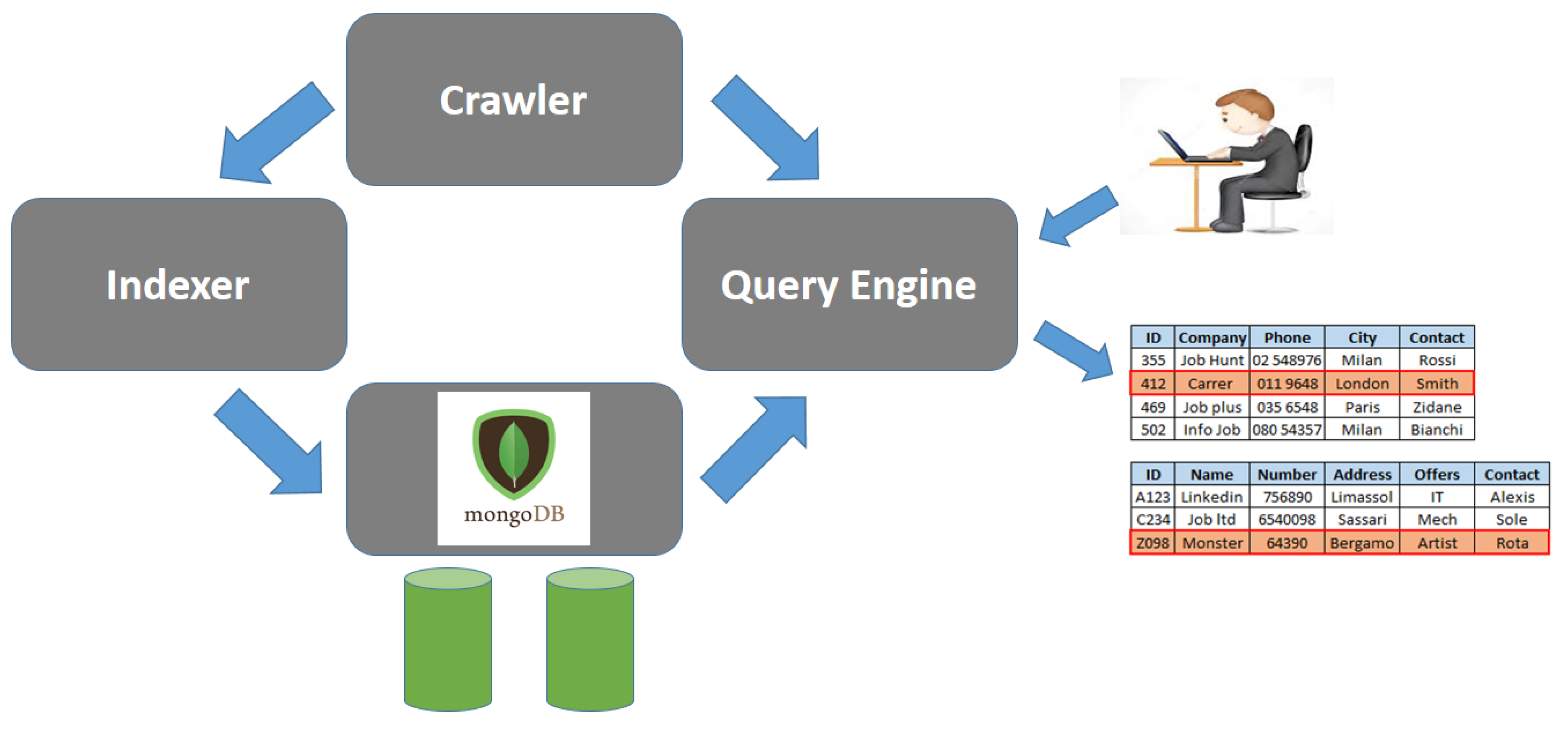
5.1. Architecture of the Hammer Prototype

In this section, we describe the architecture of the Hammer prototype. The prototype, implemented in Java, is composed by two main components, as shown in Figure 2: the Indexer and the Query Engine. Two service components complete the architecture: the Crawler and the MongoDB NoSQL database management system.

• The Indexer gets meta-data concerning data sets, without downloading the instances, and builds an Inverted Index; at the same time, the catalog of the corpus is built. Both the catalog and the inverted index are stored as collections of JSON objects within a MongoDB database.
• The Query Engine is exploited by users to actually retrieve data sets. The query is processed on the basis of the inverted index and meta-data stored in MongoDB. For data sets matching the query or some neighbour query, their instances are actually retrieved and filtered, in order to produce the output results.
• The Crawler is a service component exploited both by the indexer and by the query engine to access the Open Data portal, in order to get either meta-data about published data sets or instances.
• MongoDB NoSQL DBMS provides storage support. We decided to adopt it due to the flexibility provided by the fact that it stores JSON objects in heterogeneous collections in a native way; this way, the prototype can be easily evolved and the database can be easily adapted.

Focusing on the query engine, the internal architecture is organized in blocks, as depicted in Figure 3. The query engine is organized as a pool of Executors: each executor is responsible for performing one or two of the steps that constitute the retrieval technique presented in Section 3.3. Executors are organized in a processing pipeline, as depicted in Figure 3: the output of one executor is the input for the next one. On the left-hand side, we depicted the meta-data catalog stored within the MongoDB database; on the right-hand side, we depicted the inverted index, stored within the MongoDB database as well. In particular, the figure shows which executor exploits the catalog and/or the inverted index. Finally, notice in the bottom right corner of Figure 3, the Crawler: it is exploited by the last executor to get instances of data sets selected by the Step 4/5 Executor.

The development of the Hammer prototype evolved step by step: in the very early version, the prototype was designed as a single process tool. Then, we identified Step4/5 Executor as the critical executor as far as performances are concerned; consequently, we mainly modified the above-mentioned executor in order to exploit the Map-Reduce paradigm, by means of the Hadoop framework; then, Hadoop was replaced by the Spark framework. Finally, the algorithms were re-implemented by exploiting high-level abstractions provided by Spark.

5.2. Step 4/5 Executor: Basic Algorithm

Algorithm 1 reports the pseudo-code of the algorithm implemented within the Step4/5 Executor. The procedure is divided in two parts: in the first part, the set of data sets that satisfy at least one query $nq\in Q$ (the set of queries to process) is generated; in the second part (line 4), the final set of data sets is generated, such that their relevance measure $rm$ is greater than the minimum threshold $th\_rm$.

	Algorithm 1: Algorithm for Step 4.
	Procedure Step4/5_Executor(Q, $th\_krm$, $th\_rm$)
	Begin
1.	MongoDB_Clear_FoundDS()
2.	For Each $q\in Q$ do
3.	Process_Query(q, $th\_krm$)
	End For Each
4.	Evaluate_RM()
	End Procedure

The main data structure we adopt in the algorithm is the data set descriptor   

$$ds:(\mathtt{ds}\_\mathtt{id},\mathtt{W}:[(\mathtt{t},\mathtt{w})],\mathtt{krm},\mathtt{rm},q),$$

where ds_id is the data set identifier. W is a vector of term weights, where each element is a pair that associates a term t with its weight w (to compute the cosine similarity with respect to a query). krm is the keyword relevance measure (obtained by applying the VSM approach); rm is the best relevance measure and q is the query for which the best relevance measure is obtained.

We now present the algorithm in detail:

• At line 1, function MongoDB_Clear_FoundDS is called. It resets the content of a MongoDB collection called FoundDS: this collection has to store data set descriptors that satisfy at least one query $q\in Q$.
• The For Each loop on line 2 calls (line 3) procedure Process_Query for each query $q\in Q$. This procedure stores data set descriptors possibly found for query q in the MongoDB collection FoundDS.
• Algorithm 2 reports the pseudo-code of procedure Process_Query, which actually implements Step 4, for each single query $q\in Q$. We now describe its work in detail:
  • The procedure receives a query q and the minimum threshold for the keyword relevance measure $th\_krm$.
  • On line 2, the set $DS$ of data set descriptors is set to be empty. Furthermore, on line 3, function MongoDB_Get_FoundDS gets the set of data set descriptors already found for previous processed queries in Q.
  • The For Each loop on line 4 iterates for each term t in the set of terms $q.terms$ extracted for query q by Step 3 Executor.
    In particular, for each term t, the loop queries the inverted index stored within a MongoDB collection: function MongoDB_DS_for_term_Except queries the inverted index and returns the set of data set descriptors that contain term t; however, data sets already present in collection FoundDS are not retrieved by the function, in order to optimize the process: in fact, if a data set has been already found by a previous query, there is no need to consider it again in Step 4.
    Specifically, the If instruction on line 5 assigns the content of the set of data set descriptors retrieved from the inverted index directly to $DS$ if $DS$ is empty (for the first processed term); otherwise (Else branch on line 7), the new set of data set descriptors retrieved from the inverted index is intersected with the previous one. Only data sets common to both operands of ∩ have a descriptor in its output: consequently, $DS$ progressively narrows at each iteration.
    Finally, line 8 checks if the set $DS$ is empty: if this happens, it means that no data sets satisfying the query are in the corpus.
  • Once completed the first For Each loop, it is necessary to evaluate the keyword relevance measure for each data set in $DS$. Line 9 sets to empty the set of selected data sets $selectedDS$.
  • The loop on line 10 actually makes the computation of the keyword relevance measure $krm$ for each data set in $DS$. On line 11, the cosine similarity between terms in data set $ds$ (vector W) and terms in the query q is computed (by function CosineSimilarity).
    On line 12, the If instruction compares $ds.\mathtt{krm}$ with the threshold $th\_krm$: if the former is greater than or equal to the latter, the descriptor $ds$ is added to the set $SelectedDS$; otherwise, it is discarded.
  • Finally, line 14 checks if the set $SelectedDS$ is not empty: if so, the set of descriptors contained in $SelectedDS$ is appended to the MongoDB colelction FoundDS by procedure MongoDB_Add_FoundDS. This terminates procedure Process_Query.
• Let us come back to procedure Step4/5_Executor. After Step 4 is concluded, Step 5 is performed on line 4, by calling procedure Evaluate_RM, reported in Algorithm 3. It is described in detail hereafter:

  -

  The goal of this procedure is computing the Schema Fitting Degree (r sfd) for all data sets selected by Step 4, in order to compute the overall relevance measure $rm$. Similarly to Step 4, descriptors of data sets to work on are stored in the MongoDB collection named FoundDS, while descriptors of data sets to produce as output of the step are stored in the MongoDB collection called ResultDS. Line 1 calls procedure MongoDB_Clear_ResultDS to clear this collection.

  -

  Before starting the iterative process, line 2 initializes the set of data set descriptors to produce as output ($ResultDS$); line 3 reads the set of data set descriptors produced by Step 4 from the MongoDB collection FoundDS.

  -

  The For Each loop on line 4 operates on each data set descriptor, in order to evaluate the best relevance measure $rm$; before starting the inner loop, line 8 reads the schema of the data set from the catalog stored in MongoDB.

  -

  The inner loop on line 7 evaluates the data set against each query $q\in Q$.

  Specifically, line 8 computes the relevance measure by calling function Compute_SFD_and_RM, that computes the sfd and, based on it, the relevance measure rm, which is assigned to variable $new\_rm$.

  Line 9 compares this value with the former best value for the data set and, if the new value is greater than the old one, it becomes (line 10) the new best value and (line 11) the data set is associated with the corresponding query.

  -

  The last action of the outer loop is the comparison of the relevance measure with respect to the threshold $th\_rm$: if the measure is greater than or equal to the threshold (line 12), the data set descriptor is added to the output set $ResultDS$ (Line 13).

  -

  Finally, after the outer loop, if the set $ResultDS$ is not empty (Line 14), it is stored to the ResultDS collection in MongoDB.

	Algorithm 2: Procedure for extracting relevant data sets for a query.
	Procedure Process_Query(q, $thh\_krm$)
	Begin
1.	DS: set-of $ds:(\mathtt{ids}\_\mathtt{d},\mathtt{W}:[(\mathtt{t},\mathtt{w})],\mathtt{krm})$
2.	$DS$:= ∅
3.	$FoundDS=$MongoDB_Get_FoundDS()
4.	For Each $t\in q.terms$ do
5.	If $DS=\varnothing$ Then
6.	$DS=$MongoDB_DS_for_term_Except(t, $FoundDS$)
	Else
7.	$DS=DS\cap$ MongoDB_DS_for_term_Except(t, $FoundDS$)
	End If
8.	if $DS=\varnothing$ Then End Procedure
	End For Each
9.	$SelectedDS=\varnothing$
10.	For Each $ds\in DS$ do
11.	$ds.\mathtt{krm}=$CosineSimilarity($q.W$, $ds.\mathtt{W}$)
12.	If $ds.\mathtt{krm}\ge th\_krm$ Then
13.	$SelectedDS=SelectedDS\cup \left\{ds\right\}$
	End If
	End For Each
14.	If $SelectedDS\ne \varnothing$ Then
15.	MongoDB_Add_FoundDS($SelectedDS$)
	End If
	End Procedure

	Algorithm 3: Pseudo-code of procedure Evaluate_RM, performing Step 5.
	Procedure Evaluate_RM(Q, $th\_rm$)
	Begin
1.	MongoDB_Clear_ResultDS()
2.	$ResultDS:=\varnothing$
3.	$FoundDS:=$MongoDB_Get_FoundDS()
4.	For Each $ds\in FoundDS$ do
5.	$ds\_schema=$MongoDB_Get_Ds_Schema($ds.\mathtt{ds}\_\mathtt{id}$)
6.	$ds.\mathtt{rm}:=0$
7.	For Each $q\in Q$ do
8.	$new\_rm:=$Compute_SFD_and_RM($ds$, $ds\_schema$, q)
9.	If $ds.\mathtt{rm}<new\_rm$ Then
10.	$ds.\mathtt{rm}:=new\_rm$
11.	$ds.\mathtt{q}:=q$
	End If
	End For Each
12.	If $ds.\mathtt{rm}\ge th\_rm$ do
13.	$ResultDS:=ResultDS\cup \left\{ds\right\}$
	End If
	End For Each
14.	If $ResultDS\ne \varnothing$ Then
15.	MongoDB_Save_ResultDS(ResultDS)
	End If
	End Procedure

5.3. Evolving Step4/5 Executor toward Map-Reduce

The work performed by Step4/5 Executor is time-consuming, especially when the number of queries to process is large, as well as when the number of indexed data sets is only a few thousands (see Section 6). This motivates the introduction of the Map-Reduce approach, to try to improve performance.

We decided to adopt a lazy strategy, in order to evaluate the impact of the minimal changes necessary to transform the single-process version of Step4/5 Executor (Algorithm 1) into a Map-Reduce algorithm:

• The first part of procedure Step4/5_Executor (lines from 1 to 3), which performs Step 4, becomes the Map phase: each Map task executes procedure Process_Query on one single query. Consequently, the number of parallel tasks coincides with the number of queries in Q.
• The second part of procedure Step4/5_Executor (line 4) becomes the Reduce phase: results produced by the Map phase are collected and evaluated against queries in Q, by calling procedure Evaluate_RM.

In order to activate Map and Reduce tasks, without relying on any specific framework, we make use of two pseudo-primitives: Schedule_Map_Task and Schedule_Reduce_Task. The former pseudo- primitive schedules a Map task, by specifying the procedure to call; the latter pseudo-primitive schedules a Reduce task at the end of all previously scheduled Map tasks, by specifying the procedure to execute.

Algorithm 4 shows the modified versions of procedure Step4/5_Executor. Step 4 is always performed by lines 2 and 3; however, on line 3, procedure Process_Query is no longer called directly, while it is scheduled as a Map task. Similarly, on line 4, Step 5 is performed, but function Evaluate_RM is now scheduled as a Reduce task, in order to be executed when all Map tasks terminate.

We developed two distinct implementations, one based on the Hadoop framework, one based on the Spark framework.

Notice that we decided to adopt this strategy because we wanted to study the effect of the simplest transformation of the algorithm, without changing its structure. In fact, the reader can see that it was already naturally structured to be parallelized. This way, we can answer the questions: what is the effect of parallelization? Is Map-Reduce capable of fastening algorithms that were not thought to become Map-Reduce algorithms? Refer to Section 6 and Section 7 for the answers.

	Algorithm 4: Generic Map-Reduce version of Step4/5_Executor.
	Procedure Step4/5_Executor(Q, $th\_krm$, $th\_rm$)
	Begin
1.	MongoDB_Clear_FoundDS()
2.	For Each $q\in Q$ do
3.	Schedule_Map_Task(ProcessQuery(q, $th\_krm$))
	End For Each
4.	Schedule_Reduce_Task(Evaluate_RM(Q, $th\_rm$))
	End Procedure

5.4. Enhancing Step 4: Exploiting High-Level Abstractions Provided by Spark

To continue the study about the impact of the Map-Reduce approach on our query engine, we developed an enhanced version of Step4/5 Executor, in which Map and Reduce tasks do not interact with MongoDB. This version exploits a high-level abstraction provided by Spark, called Dataset, that has been introduced in version 2 of Spark; Spark datasets are developed on top of RDD. The advantage of this abstraction is simplicity: as we will show, the program is written in a very simple way. In the rest of the paper, with the term sdataset, we will refer to Spark datasets, while, with data set, we will refer to a data set in the corpus C.

Algorithm 5 reports the enhanced Spark version of procedure Step4/5_Executor. The procedure has two extra parameters, i.e., I and D: I is a sdataset containing the inverted index; D is an sdataset containing the catalog of the corpus; now, Q is a sdataset, still containing queries.

Table 1. Structure of Spark datasets in procedure Step4/5_Executor reported in Algorithm 5.

Sdataset	Set-of
Q	<q_id, KW: vector-of(<kw, w>)>
I	<term, DS: vector-of(< ds_id>) >
D	<ds_id, schema: vector-of(<term, role, weight>)
$q\_k\_ds$	<q_id, kw, ds_id>
$q\_ds$	<q_id, ds_id, K: vector-of(<kw, w>)>
$q\_ds\_krm$	<q_id, ds_id, krm>

reports the structure of crucial sdatasets in the procedure. As the reader can see, they are non-flat tables (non 1-NF, non first normal form). In particular, a query in Q contains vector KW, that describes keywords in the query (field kw) with the corresponding weight (field w). Similarly, each element in I is a tuple that associates a term with the vector DS of data set identifiers. D associates a data set identifier ds_id with a vector schema, where each tuple describes a term in the schema, its role (e.g., data set name, field, etc.) and its weight (that depends on the role).

Let us consider now the procedure Step4/5_Executor. Algorithm 5 reports the pseudo-code of the Java-hosted Spark procedure that we implemented (by means of the pseudo-code, we avoid useless technicalities).

Lines from 1 to 3 correspond to Step 4, while lines 4 and 5 correspond to Step 5.

	Algorithm 5: Procedure Step4/5_Executor implemented as a Spark v2 program.
	Procedure Step4/5_Executor(Q, $th\_krm$, $th\_rm$, I, D)
	Begin
1.	$q\_k\_ds$ =
1a.	Q.select("q_id", explode("KW"))
1b.	.join(I on"kw==term")
1c.	.select("q_id", "kw", "w", explode("ds_id"));
2.	$q\_ds$:= $q\_k\_ds$.groupBy("q_id", "ds_id").aggregate("kw").as("K")
3.	$q\_ds\_krm$:=
3a.	$q\_ds$.join(Q on "q_id")
3b.	.map(t ->{ t.krm:=CosineSimilarity(q.KW, q.W, q.K) })
3c.	.filter("krm ≥ $tr\_krm$"))
3d.	.select("q_id", "ds_id", "krm")
3e.	.collect()
4.	$q\_ds\_rm$:=
4a.	$q\_ds\_krm$.join(Don"ds_id")
4b.	.map(e->{e.rm:=Compute_RM(e.krm, e.schema, e.KW)})
4c.	.filter("rm ≥ $th\_rm$")
5.	$ResyktDS$:=
5a.	$q\_ds\_rm$.groupBy("q_id", "ds_id").max("rm")
5b.	.join($q\_ds\_rm$on"q_id and ds_id and rm").select("ds_id", "rm", "q_id")
5c.	.collect()
	End Procedure

• On line 1, the temporary sdataset named $q\_k\_ds$ is computed: it has to contain tuples associating a query (by its identifier q_id) with a keyword kw and a data set (by its identifier ds_id) that contains that keyword. See the structure in Table 1.
  Line 1a flattens vector KW in tuples describing queries: this is necessary to associate the query with data set identifiers through the inverted index. Notice the explode operation in the select operation, which transforms the nested tuples into flat tuples (one tuple for each element in the vector).
  Line 1b. performs a join with the sdataset I, that contains the inverted index (notice the join condition after the on). The resulting table contains vector DS, with data set identifiers: for this reason, the select operation on line 1c exploits the explode operation, in order to flatten the tuples by unnesting fields ds_id.
• Line 2 prepares sdataset $q\_k\_ds$ in order to aggregate common terms between a query and a data set.
  Specifically, a groupBy operation is performed, in order to group tuples having the same q_id and ds_id. The subsequent aggregate operation aggregates single values of field kw into one single vector, which is given the name K.
  The resulting temporary sdataset is named $q\_ds$; its structure is shown in Table 1.
• The actual computation of the $krm$ value (keyword relevance measure) for each data set with respect to a query is computed on line 3.
  Specifically, line 3a joins the previous temporary sdataset $q\_ds$ with sdatasetQ, in order to get again the KW vector of keywords with weights. This vector is necessary to compute the cosine similarity.
  Line 3b actually computes the cosine similarity, which is the value of the new field krm. This is performed by explicitly performing a nap operation: for each tuple handled by means of the iterator t, the code within braces after the -> is executed. This code calls function CosineSimilarity to compute the relevance measure and extend the tuple with field krm.
  Notice that the programmer explicitly schedules Map tasks. Nevertheless, it is not excluded that other operations are scheduled as Map tasks, such as unnesting: this is autonomously performed by the framework.
  The operation ends by filtering tuples with value of field krm greater than or equal to the minimum threshold $th\_krm$ (line 3c) and by subsequently restructuring the sdataset (line 3d).
  Notice the final collect operation: this is necessary to force Spark to actually perform the computation. In fact, Spark does not execute the program until it is not forced to do that. The collect operation is one possibility.

At this point, lines 4 and 5 perform Step 5.

• In order to evaluate the Schema Fitting Degree and, on its basis, the relevance measure $rm$, it is necessary to retrieve the schema of each data set. Data set schemas are stored in the sdatasetD.
  On line 4a, the temporary data set obtained by line 3, named $q\_ds\_krm$, is joined with sdatasetD (the join condition is equality of fields with the same name).
  Map tasks are scheduled: on each tuple e (iterator over the sdataset) function Compute_RM is called. This function receives the keyword relevance measure krm, the schema of the data set, the vector KW of keywords in the query. A new field named rm is added to the tuple handled by e.
  On line 4c, only tuples with value of field rm greater than or equal to the minimum threshold $th\_rm$ are selected. These become the new temporary sdataset $q\_ds\_rm$.
• Finally, line 5 provides the final sdataset $ResultDS$. Since in the sdataset $q\_ds\_rm$ the same data set might be associated with more than one query, in order to be compliant with the other implementations, it is necessary to take the best association.
  Consequently, line 5a groups tuples on the basis of field ds_id; then, it computes the maximum value for field rm.
  Line 5b joins tuples describing groups with original tuples in sdataset $q\_ds\_rm$, on the basis of the value of the common field rm: this way, the query identifier q_id is associated with ds_id.

The reader can notice that, by adopting sdatasets, the procedure has become more functional and less procedural. This is a very important advantage provided by sdatasets.

Furthermore, programmers do not have to worry about explicit parallelization of tasks: high-level operations may implicitly be executed as Map-Reduce operations by the framework, in a transparent way. Consequently, programmers focus only on the business logic of the problem, being aware that, were possible, the computation will be parallelized.

5.5. Other Executors Implemented by Means of Map-Reduce

Other executors in the Hammer prototype have been parallelized by means of the Map-Reduce approach. Since they are less critical than Step4/5 Executor, we have not discussed them.

Specifically, Step 2 Executor is implemented too on the basis of the Map-Reduce approach: in fact, given the set of alternative terms computed by Step 1 Executor, neighbor queries can be generated in a parallel way. Since this part is not critical, we do not describe it.

In addition, Step 6 Executor has been parallelized by means of Map-Reduce. In this step, instances of selected data sets are downloaded from the Open Data portal and filtered. As shown in [3], the Map-Reduce approach helps with parallelizing this task.

6. Experimental Campaign

In this section, we present the results of the experimental campaign we conducted to evaluate the benefits provided by adopting the Map-Reduce approach. Specifically, we compare execution times exhibited by all the implementations discussed in Section 5.

Recall that, in this paper, we focus on efficiency; readers interested in effectiveness (evaluated in terms of recall and precision) of the retrieval technique can refer to [1,2].

6.1. Experimental Settings

Experiments concern performances exhibited by the query engine at query time. We used three execution environments and nine configurations of the Hammer query engine.

6.1.1. Execution Environments

Table 2. Execution environments.

Environment	Technology	Nodes	Virtual CPUs	Total RAM
$En{v}_1$	Hadoop	2	6	6 GB
$En{v}_2$	Spark	1	3	3 GB
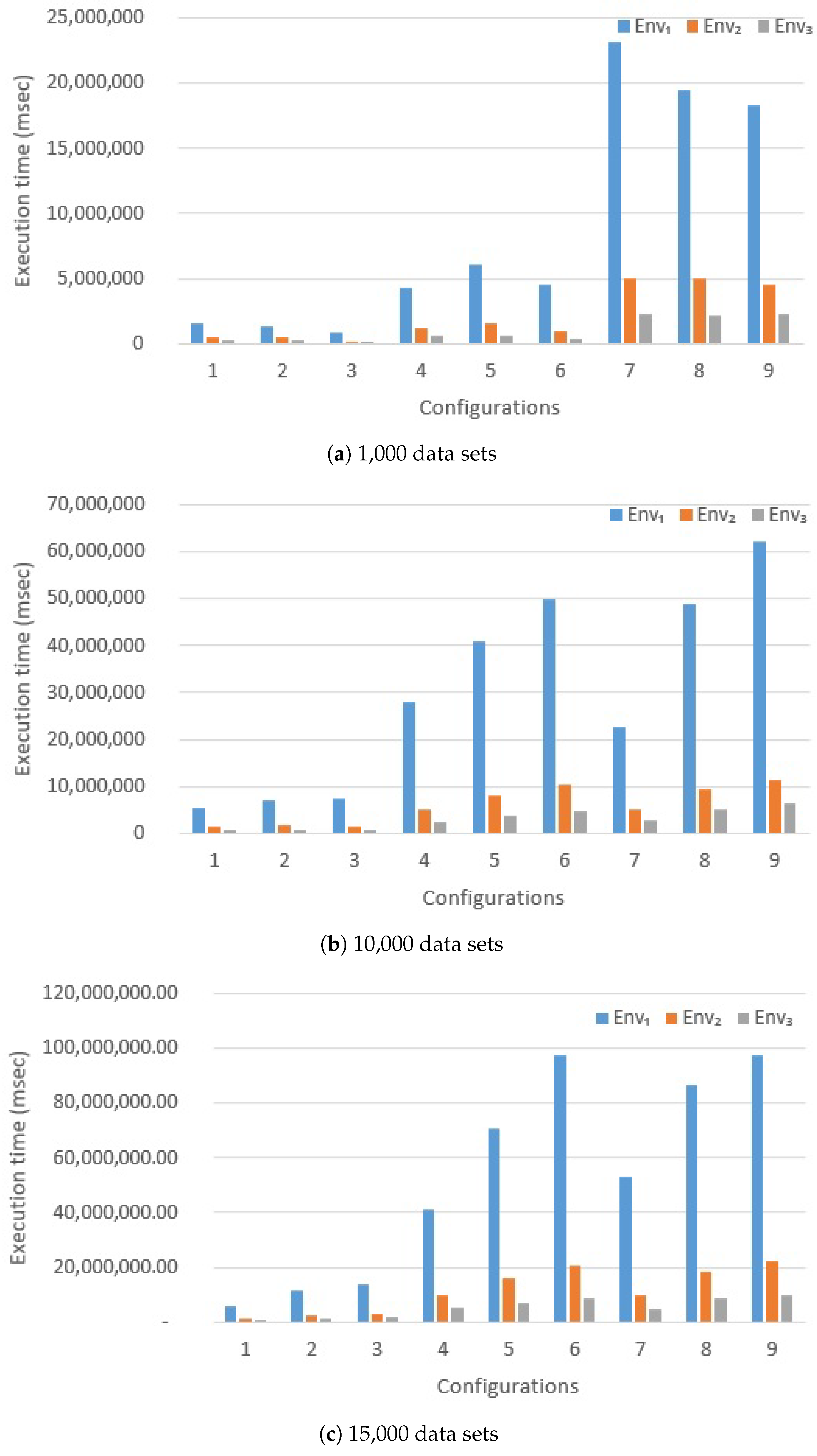
$En{v}_3$	Spark	2	6	6 GB

reports the three different execution environments we set up. The environments are hosted on Amazon AWS infrastructure.

• Environment $En{v}_1$ is a cluster of two nodes powered by Hadoop technology; each node has 3 GB RAM shared among three virtual CPUs; the total amount of RAM available for executors is 6 GB.
• Environment $En{v}_2$ is a single node powered by Spark technology (standalone mode); the total RAM is 3 GB, shared among three virtual CPUs.
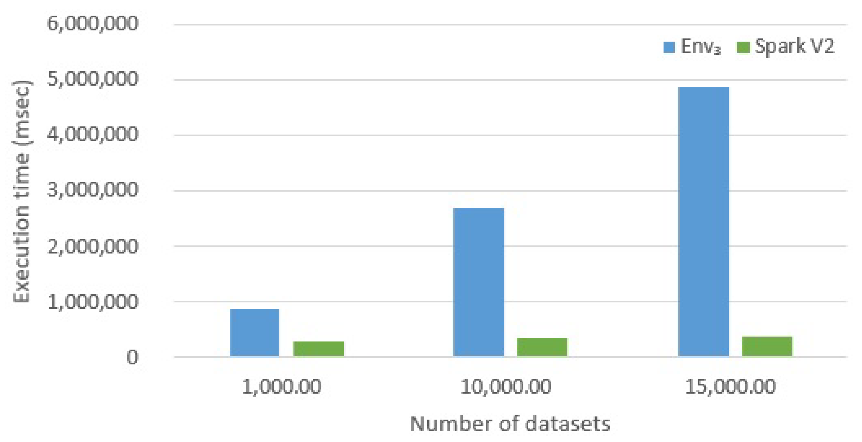
• Environment $En{v}_3$ is a cluster of two nodes powered by Spark technology; each node has 3 GB RAM shared among three virtual CPUs; thus, the cluster is equipped with six virtual CPUs that share 6 GB RAM.

6.1.2. Configurations of the Hammer Query Engine

Table 3. Configurations of the Hammer query engine.

Configuration	max_neigh	th_krm	th_rm	th_sim
$Con{f}_1$	10	0.2	0.2	0.9
$Con{f}_2$	10	0.2	0.2	0.8
$Con{f}_3$	10	0.3	0.3	0.9
$Con{f}_4$	100	0.2	0.2	0.9
$Con{f}_5$	100	0.2	0.2	0.8
$Con{f}_6$	100	0.3	0.3	0.9
$Con{f}_7$	1000	0.2	0.2	0.9
$Con{f}_8$	1000	0.2	0.2	0.8
$Con{f}_9$	1000	0.3	0.3	0.9

summarizes the nine different configurations we experimented for the Hanner query engine.

• Parameter max_neigh determines the maximum number of neighbor queries to generate from the original query q. We chose three values: maximum 10 neighbor queries (configurations $Con{f}_1$, $Con{f}_2$ and $Con{f}_3$), maximum 100 neighbor queries (configurations $Con{f}_4$, $Con{f}_5$ and $Con{f}_6$) and maximum 1000 neighbor queries (configurations $Con{f}_7$, $Con{f}_8$ and $Con{f}_9$). The greater the value, the harder the work to perform to evaluate each query to process against the inverted index.
• Parameter th_krm determines the minimum threshold for selecting data sets based on the VSM method, on the basis of information present in the inverted index (Step 4 of the retrieval technique, see Section 3.3). We considered two different values: 0.2 (for configurations $Con{f}_1$ and $Con{f}_2$, $Con{f}_4$ and $Con{f}_5$, $Con{f}_7$ and $Con{f}_8$) and 0.3 (for configurations $Con{f}_3$, $Con{f}_6$ and $Con{f}_9$). The smaller its value, the greater the number of data sets to retrieve and to process.
• Parameter th_rm determines the minimum threshold for selecting data sets based on the overall relevance measure $rm$ (Step 5 of the retrieval technique, see Section 3.3). We considered two different values: 0.2 (for configurations $Con{f}_1$ and $Con{f}_2$, $Con{f}_4$ and $Con{f}_5$, $Con{f}_7$ and $Con{f}_8$) and 0.3 (for configurations $Con{f}_3$, $Con{f}_6$ and $Con{f}_9$). The smaller its value, the greater the number of data sets to retrieve and to process.
• Parameter th_sim denotes the minimum threshold of string similarity used to select alternative terms on the basis of string similarity (Step 1 of the retrieval technique, see Section 3.3). We considered two different values: 0.9 (for configurations $Con{f}_1$ and $Con{f}_3$, $Con{f}_4$ and $Con{f}_6$, $Con{f}_7$ and $Con{f}_9$) and 0.8 (for configurations $Con{f}_2$, $Con{f}_5$ and $Con{f}_8$). The lower the value, the larger the number of alternative terms retrieved on the basis of string similarity. However, for each term in the original query, we always limit the maximum number of alternative terms chosen on the basis of string similarity to 3.

6.1.3. Sample Corpora

In order to perform experiments, we considered the www.data.gov Open Data portal. It is the official Open Data portal of the U.S. Government. The portal plays the role of repository for federal, state, and local governments. Currently (2018), about 300,000 data sets are published, in various formats. For our purpose, we built three sample corpora of data sets extracted from data.gov: the first contains 1000 data sets; the second contains 10,000 data sets; the third contains 15,000 data sets.

After indexing of meta-data, the inverted index contains a significant number of entries. In particular, for the corpus containing 1000 data sets, the inverted index contains 13,916 terms and 127,396 pairs (term, data set id). For the corpus containing 10,000 data sets, the inverted index contains 52,865 terms and 1,105,390 pairs (term, data set id). For the corpus with 15,000 data sets, the inverted index contains 71,159 terms and 1,794,330 pairs (term, data set id).

6.1.4. Query

The query chosen to perform tests is the following:

$q:<$dn = [cities],

   P $=\{$ [city], [population], [outcomes]},

   sc $=($ [census] = 2017$)>$.

The query was chosen in order to retrieve at least one data set from within the sample corpora used to perform tests.

6.2. Results

Now, we are ready to present the results of our performance analysis. Execution times, obtained for the Single-Process version of the algorithm (in the rest of the paper denoted as NO MR, for simplicity), are reported in

Table 4. Execution times for the corpora of 1000–10,000–15,000 data sets for version without Map-Reduce of the algorithm.

1000 Data Sets	Step 1	Step 2	Step 3	Step 4	Step 5	Step 6	Total
$Con{f}_1$	69,699	150	5277	1,410,492	158,891	610,013	2,254,522
$Con{f}_2$	83,689	102	1844	1,001,012	171,160	556,510	1,814,317
$Con{f}_3$	137,742	143	1440	895,619	152,791	27,897	1,215,632
$Con{f}_4$	128,504	163	1082	5,075,391	79,785	554,400	5,839,325
$Con{f}_5$	159,436	109	1884	6,796,491	836,515	583,513	8,377,948
$Con{f}_6$	133,152	125	987	5,821,900	73,433	49,266	6,078,863
$Con{f}_7$	164,107	166	1206	29,952,490	55,401	463,736	30,637,106
$Con{f}_8$	173,785	127	1649	24,480,779	694,722	651,068	26,002,130
$Con{f}_9$	133,349	127	1273	23,848,456	84,014	46,749	24,113,968
10,000 Data Sets	Step 1	Step 2	Step 3	Step 4	Step 5	Step 6	Total
$Con{f}_1$	125,162	133	8289	6,247,375	1,774,413	494,387	8,649,759
$Con{f}_2$	145,730	142	1442	8,940,382	1,793,918	563,101	11,444,715
$Con{f}_3$	257,793	75	995	11,585,182	559,855	111,507	12,515,407
$Con{f}_4$	265,262	190	1277	44,882,444	1,374,816	464,295	46,988,284
$Con{f}_5$	127,091	125	1615	54,313,736	11,374,301	521,144	66,338,012
$Con{f}_6$	94,438	75	847	84,234,220	349,861	197,854	84,877,295
$Con{f}_7$	87,629	64	1238	36,259,183	1,250,844	349,380	37,948,338
$Con{f}_8$	157,812	117	2051	66,990,740	12,107,156	746,812	80,004,688
$Con{f}_9$	204,534	129	1386	104,930,839	505,326	163,578	105,805,792
15,000 Data Sets	Step 1	Step 2	Step 3	Step 4	Step 5	Step 6	Total
$Con{f}_1$	109,365	50	6263	6,367,932	805,445	683,549	7,972,604
$Con{f}_2$	130,563	385	979	13,668,545	875,351	690,821	15,366,644
$Con{f}_3$	224,922	139	1026	16,693,411	1,097,360	122,420	18,139,278
$Con{f}_4$	294,392	153	1091	51,177,294	2,852,516	523,599	54,849,045
$Con{f}_5$	170,759	193	1750	72,817,934	20,378,100	673,203	94,041,939
$Con{f}_6$	103,225	72	661	128,535,201	689,922	213,775	129,542,856
$Con{f}_7$	71,493	93	1719	67,185,486	3,118,435	457,630	70,834,856
$Con{f}_8$	190,613	139	2486	90,892,440	23,580,870	771,655	115,438,203
$Con{f}_9$	161,401	198	1787	128,640,058	1,163,036	242,773	130,209,253

; notice that the table is divided in three parts, each one (as denoted in the upper left corner) corresponds to a different number of indexed data sets (1000, 10,000 and 15,000).

Execution times for the first Map-Reduce version of the algorithm (described in Section 5.3) are reported in

Table 5. Execution times for the corpus of 1000 data sets (first Map-Reduce version).

${\mathit{Env}}_1$	Step 1	Step 2	Step 3	Step 4	Step 5	Step 6	Total
$Con{f}_1$	49,954	105	3789	1,067,387	89,904	419,777	1,630,916
$Con{f}_2$	59,981	71	1324	757,514	96,846	382,959	1,298,695
$Con{f}_3$	98,722	100	1034	677,758	86,452	19,197	883,263
$Con{f}_4$	92,101	114	777	3,840,793	45,144	381,507	4,360,436
$Con{f}_5$	114,270	76	1353	5,143,232	473,317	401,541	6,133,789
$Con{f}_6$	95,432	87	709	4,405,712	41,550	33,902	4,577,392
$Con{f}_7$	117,618	116	866	22,666,491	31,347	319,117	23,135,555
$Con{f}_8$	124,554	89	1184	18,525,784	393,088	448,029	19,492,728
$Con{f}_9$	95,573	89	914	18,047,275	47,537	32,170	18,223,558
${\mathit{Env}}_{\mathbf{2}}$	Step 1	Step 2	Step 3	Step 4	Step 5	Step 6	Total
$Con{f}_1$	12,170	64	819	182,765	15,345	341,675	552,838
$Con{f}_2$	12,144	60	225	172,772	16,442	344,312	545,955
$Con{f}_3$	22,020	86	205	123,625	15,536	16,169	177,641
$Con{f}_4$	19,871	83	141	890,814	10,057	305,142	1,226,108
$Con{f}_5$	22,414	49	261	1,110,737	83,602	337,270	1,554,333
$Con{f}_6$	16,904	65	127	941,497	9991	28,069	996,653
$Con{f}_7$	20,189	89	148	4,631,174	6872	304,278	4,962,750
$Con{f}_8$	23,781	59	289	4,561,780	81,840	378,912	5,046,661
$Con{f}_9$	22,619	71	156	4,445,672	11,872	27,817	4,508,207
${\mathit{Env}}_{\mathbf{3}}$	Step 1	Step 2	Step 3	Step 4	Step 5	Step 6	Total
$Con{f}_1$	6211	77	856	97,479	9511	188,150	302,284
$Con{f}_2$	6156	62	247	78,478	9512	204,319	298,774
$Con{f}_3$	11,540	102	207	64,805	10,804	7431	94,889
$Con{f}_4$	11,196	84	147	487,033	3423	101,937	603,820
$Con{f}_5$	11,051	56	285	460,746	42,592	101,783	616,513
$Con{f}_6$	8784	67	127	388,326	5643	14,703	417,650
$Con{f}_7$	11,148	99	152	2,076,886	4416	152,356	2,245,057
$Con{f}_8$	10,979	66	305	1,923,165	51,733	156,590	2,142,838
$Con{f}_9$	12,386	75	157	2,219,314	3836	13,466	2,249,234

,

Table 6. Execution times for the corpus of 10,000 data sets (first Map-Reduce version).

${\mathit{Env}}_1$	Step 1	Step 2	Step 3	Step 4	Step 5	Step 6	Total
$Con{f}_1$	96,230	85	5275	3,664,468	1,322,651	350,531	5,439,240
$Con{f}_2$	112,044	91	918	5,244,081	1,337,190	399,251	7,093,575
$Con{f}_3$	198,203	48	633	6,795,418	417,317	79,061	7,490,680
$Con{f}_4$	203,945	122	813	26,326,300	1,024,791	329,195	27,885,166
$Con{f}_5$	97,713	80	1028	31,858,330	8,478,428	369,502	40,805,081
$Con{f}_6$	72,608	48	539	49,408,525	260,787	140,283	49,882,790
$Con{f}_7$	67,373	41	788	21,268,230	932,382	247,718	22,516,532
$Con{f}_8$	121,333	75	1305	39,294,169	9,024,700	529,506	48,971,088
$Con{f}_9$	157,255	83	882	61,548,359	376,671	115,980	62,199,230
${\mathit{Env}}_{\mathbf{2}}$	Step 1	Step 2	Step 3	Step 4	Step 5	Step 6	Total
$Con{f}_1$	18,623	56	1002	901,137	280,039	344,775	1,545,632
$Con{f}_2$	19,998	68	199	968,779	291,047	356,721	1,636,812
$Con{f}_3$	39,058	46	158	1,330,173	93,359	63,953	1,526,747
$Con{f}_4$	41,487	83	173	4,392,227	183,535	307,911	4,925,416
$Con{f}_5$	19,370	62	231	6,228,201	1,479,875	349,425	8,077,164
$Con{f}_6$	16,938	29	98	10,130,264	60,038	111,021	10,318,388
$Con{f}_7$	13,047	41	189	4,684,841	191,352	214,286	5,103,756
$Con{f}_8$	25,700	61	296	7,254,463	1,704,038	411,768	9,396,326
$Con{f}_9$	27,347	75	203	11,092,073	82,351	110,652	11,312,701
${\mathit{Env}}_{\mathbf{3}}$	Step 1	Step 2	Step 3	Step 4	Step 5	Step 6	Total
$Con{f}_1$	9452	63	1050	446,641	129,776	174,026	761,008
$Con{f}_2$	9011	79	219	529,375	117,673	188,706	845,063
$Con{f}_3$	18,057	49	163	759,816	47,116	21,842	847,043
$Con{f}_4$	20,138	84	180	2,159,509	70,524	176,915	2,427,350
$Con{f}_5$	9906	72	249	2,701,601	880,321	175,523	3,767,672
$Con{f}_6$	9404	30	104	4,610,965	31,309	56,121	4,707,933
$Con{f}_7$	5712	46	190	2,661,610	71,846	105,054	2,844,458
$Con{f}_8$	13,173	66	324	4,132,891	771,158	245,783	5,163,395
$Con{f}_9$	11,117	88	208	6,224,426	30,077	66,208	6,332,124

and

Table 7. Execution times for the corpus of 15,000 data sets (first Map-Reduce version).

${\mathit{Env}}_1$	Step 1	Step 2	Step 3	Step 4	Step 5	Step 6	Total
$Con{f}_1$	79,009	29	4408	4,775,258	606,463	423,296	5,888,463
$Con{f}_2$	94,323	224	689	10,249,925	659,099	427,799	11,432,059
$Con{f}_3$	162,491	81	722	12,518,246	826,261	75,810	13,583,611
$Con{f}_4$	212,678	89	768	38,377,416	2,147,812	324,245	41,063,008
$Con{f}_5$	123,362	112	1232	54,605,547	15,343,763	416,889	70,490,905
$Con{f}_6$	74,573	42	465	96,387,450	519,479	132,383	97,114,392
$Con{f}_7$	51,649	54	1210	50,381,822	2,348,037	283,393	53,066,165
$Con{f}_8$	137,705	81	1750	68,159,465	17,755,300	477,857	86,532,158
$Con{f}_9$	116,601	115	1258	96,466,081	875,712	150,340	97,610,107
${\mathit{Env}}_{\mathbf{2}}$	Step 1	Step 2	Step 3	Step 4	Step 5	Step 6	Total
$Con{f}_1$	18,639	25	809	942,283	130,175	357,763	1,449,694
$Con{f}_2$	15,782	154	168	2,072,424	145,164	347,329	2,581,021
$Con{f}_3$	37,310	49	176	2,703,332	195,522	63,648	3,000,037
$Con{f}_4$	41,833	80	188	9,397,267	390,018	299,062	10,128,448
$Con{f}_5$	21,482	68	264	12,910,417	2,916,485	363,245	16,211,961
$Con{f}_6$	17,548	31	108	20,408,651	125,260	109,565	20,661,163
$Con{f}_7$	12,658	46	204	92,838,15	393,117	224,765	9,914,605
$Con{f}_8$	27,944	68	321	14,424,530	3,400,795	398,221	18,251,879
$Con{f}_9$	26,909	86	217	22,155,578	171,715	115,647	22,470,152
${\mathit{Env}}_{\mathbf{3}}$	Step 1	Step 2	Step 3	Step 4	Step 5	Step 6	Total
$Con{f}_1$	9762	26	879	444,505	50,496	148,585	654,253
$Con{f}_2$	7341	182	175	1,058,477	72,370	203,713	1,342,258
$Con{f}_3$	16,910	58	193	1,492,059	86,309	37,498	1,633,027
$Con{f}_4$	19,457	95	188	4,627,830	254,045	146,739	5,048,354
$Con{f}_5$	9366	80	274	5,935,994	919,258	166,406	7,031,378
$Con{f}_6$	8061	36	111	8,743,991	56,670	50,373	8,859,242
$Con{f}_7$	6615	54	221	4,272,484	246,609	105,990	4,631,973
$Con{f}_8$	11,850	80	348	7,256,341	1,255,804	135,068	8,659,491
$Con{f}_9$	11,609	93	219	9,869,213	73,973	45,676	10,000,783

. Specifically, Table 5 reports execution times for the corpus containing 1000 data sets; Table 6 reports execution times for the corpus containing 10,000 data sets; Table 7 reports execution tims for the corpus containing 15,000 data sets. All three tables are divided into three parts: the upper part is concerned with execution environment $En{v}_1$; the central part is concerned with execution environment $En{v}_2$; the lower part is concerned with execution environment $En{v}_3$.

Finally,

Table 8. Execution times for the corpus of 1000–10,000–15,000 data sets for version Spark V2.

1000 Data Sets	Step 1	Step 2	Step 3	Step 4	Step 5	Step 6	Total
$Con{f}_1$	17,231	56	307	34,855	9297	187,456	249,202
$Con{f}_2$	17,545	41	98	45,909	10,955	216,205	290,753
$Con{f}_3$	32,890	67	82	21,395	12,443	7863	74,740
$Con{f}_4$	31,910	55	58	160,793	3942	107,867	304,625
$Con{f}_5$	31,496	37	113	162,115	49,055	107,704	350,520
$Con{f}_6$	25,035	44	50	128,205	6499	15,558	175,391
$Con{f}_7$	31,773	65	60	685,682	5086	161,219	883,885
$Con{f}_8$	31,291	44	121	694,931	59,583	165,700	951,670
$Con{f}_9$	35,301	50	62	532,704	4418	14,249	586,784
10,000 Data Sets	Step 1	Step 2	Step 3	Step 4	Step 5	Step 6	Total
$Con{f}_1$	9303	68	1062	45,887	125,741	175,371	357,432
$Con{f}_2$	8869	85	221	60,440	114,015	190,165	373,795
$Con{f}_3$	17,773	53	165	28,167	45,651	22,011	113,820
$Con{f}_4$	19,821	90	182	211,685	68,331	178,282	478,391
$Con{f}_5$	9750	77	252	213,426	852,953	176,880	1,253,338
$Con{f}_6$	9256	32	105	168,783	30,336	56,555	265,067
$Con{f}_7$	5622	49	192	902,706	69,612	105,866	1,084,047
$Con{f}_8$	12,966	71	328	914,883	747,183	247,683	1,923,114
$Con{f}_9$	10,942	94	210	662,619	29,142	66,720	769,727
15,000 Data Sets	Step 1	Step 2	Step 3	Step 4	Step 5	Step 6	Total
$Con{f}_1$	10,199	25	923	48,677	49,986	156,749	266,559
$Con{f}_2$	7670	172	184	64,115	71,638	214,906	358,685
$Con{f}_3$	17,667	55	203	29,880	85,437	39,558	172,800
$Con{f}_4$	20,328	90	197	224,558	251,477	154,802	651,452
$Con{f}_5$	9785	76	288	226,405	909,965	175,549	1,322,068
$Con{f}_6$	8422	34	117	179,047	56,097	53,141	296,858
$Con{f}_7$	6911	51	232	957,602	244,116	111,814	1,320,726
$Con{f}_8$	12,380	76	366	970,519	1,243,109	142,489	2,368,939
$Con{f}_9$	12,129	88	230	594,276	73,225	48,186	728,134

reports the execution times obtained for the enhanced version of the implementation, based on sdatasets, executed on environment $En{v}_3$; in the rest of the paper, we will denote this version as Spark V2. Again, each part of the table describes execution times obtained for 1000, 10,000 and 15,000 data sets, respectively.

In all five tables, we tested the nine configurations described in Table 3 (from $Con{f}_1$ to $Con{f}_9$); execution times of each single step of the retrieval process (see Section 3.3) are reported (columns Step 1 to Step 6); column Total reports the total execution time for each configuration.

Step 4 appears to be the most time-consuming step: its execution times are always at least 10 times larger than execution times exhibited by other steps. This is not surprising because this step performs the VSM evaluation of each query to process with respect to the inverted index, in order to retrieve data sets that possibly match the query.

Nevertheless, Step 6 contributes to the total execution time significantly, even though with execution times which are, often, a tenth of Step 4. This is not surprising because Step 6 is responsible for downloading instances of data sets from the Open Data portal and filtering objects that satisfy the selection condition. Nevertheless, with execution environment $En{v}_3$ (first Map-Reduce version), it happens that Step 4 is faster than Step 6, with configurations $Con{f}_1$, $Con{f}_2$ and $Con{f}_3$; this happens only with 1000 data sets (Table 5).

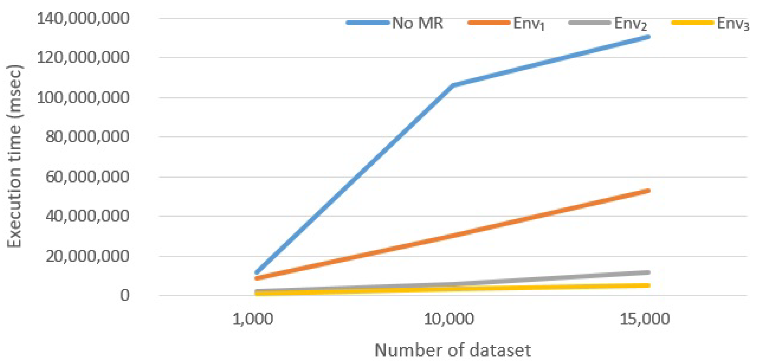
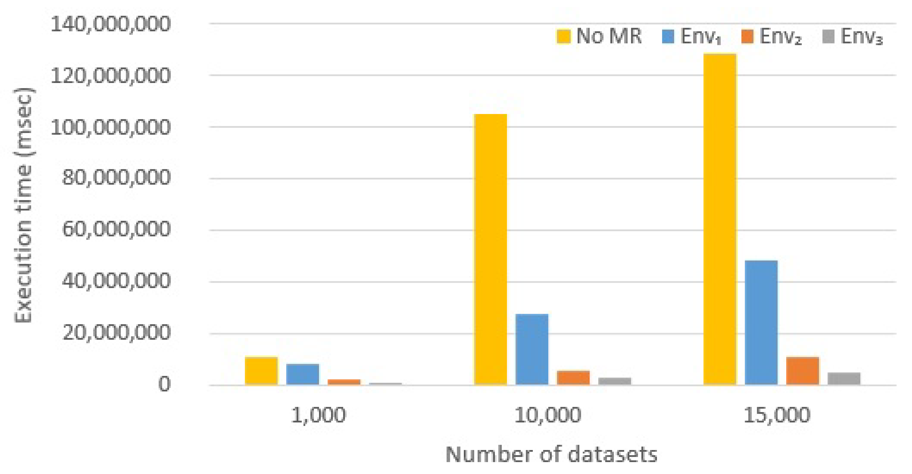
6.2.1. Effect of Introducing Map-Reduce

Let us start by evaluating the effect of introducing Map-Reduce. Figure 4 compares the overall average execution times of the No MR version (yellow line) with Hadoop and Spark versions on execution environments $En{v}_1$, $En{v}_2$ and $En{v}_3$.

Table 9. Fraction of average execution times for environment $En{v}_1$ (Hadoop technology) with respect to no Map-Reduce version.

Configuration	max_neigh	1000 Data Sets	10,000 Data Sets	15,000 Data Sets
$Con{f}_1$		72.30%	62.88%	73.86%
$Con{f}_2$	10	71.58%	61.98%	74.40%
$Con{f}_3$		72.66%	59.85%	74.89%
$Con{f}_4$		74.67%	59.34%	74.87%
$Con{f}_5$	100	73.21%	61.51%	74.96%
$Con{f}_6$		75.30%	58.77%	74.97%
$Con{f}_7$		75.51%	59.33%	74.92%
$Con{f}_8$	1000	74.97%	61.21%	74.96%
$Con{f}_9$		75.57%	58.79%	74.96%

shows the percentage of total execution times of $En{v}_1$ with respect to version No MR, for the nine different configurations. Figure 5 compares only average execution times exhibited by Step 4 only (again, the yellow bars correspond to version No MR).

Notice that, without changing the structure of the algorithm (as described in Section 5.3), the introduction of Map-Reduce is beneficial. In fact, even though the Hadoop version is the slowest among the Map-Reduce based ones, parallelism is effective in reducing execution times. Even though we can guess that the bottleneck of the process is accessing MongoDB server, the gain is from 30 to 40%.

6.2.2. Hadoop vs. Spark Comparison

We now compare performance exhibited by the basic Map-Reduce version of the algorithm (described in Section 5.3), executed on environments $En{v}_1$ (Hadoop), $En{v}_2$ (Spark) and $En{v}_3$ (Spark).

We now focus on execution times shown by Step 4 of the retrieval technique (Section 3.3). Figure 5 depicts the average execution times of Step 4; blue bars correspond to environment $En{v}_1$; red bars correspond to environment $En{v}_2$ and grey bars correspond to environment $En{v}_3$. The aggregated behavior shown in the figure is the same shown in Figure 4 for the average total execution times; this confirms that the general behavior is dominated by Step 4, i.e., retrieval of data sets that match the queries to process: the greater the number of indexed data sets, the greater the execution times to find the matching ones.

However, we can do an interesting observation (for both Figure 4 and Figure 5): the growth of the data sets of a factor 10 (from 1000 data sets to 10,000 data sets) does not cause a growth of execution times of a factor 10, but only around 3. This is true for all three of the environments.

In contrast, further increasing the number of data sets of a factor 1.5 (from 10,000 data sets to 15,000 data sets), execution times grow with a factor 2. This means that the way the Map-Reduce approach parallelizes the execution is the same with both technologies (notice that both environments $En{v}_1$ and $En{v}_3$ have the same amount of RAM). Thus, we can conclude that Spark is much more efficient than Hadoop due to critical implementation choices, concerning the way data are distributed to jobs (i.e., the main-memory RDDs).

The reader can also observe

Table 10. Fraction of average execution times for environments $En{v}_2$ and $En{v}_3$ (Spark technology) with respect to execution times for environment $En{v}_1$ (Hadoop technology).

${\mathit{Env}}_2$	max_neigh	1000 Data Sets	10,000 Data Sets	15,000 Data Sets
$Con{f}_1$		33.90%	28.42%	24.62%
$Con{f}_2$	10	42.04%	23.07%	22.58%
$Con{f}_3$		20.11%	20.38%	22.09%
$Con{f}_4$		28.12%	17.66%	24.67%
$Con{f}_5$	100	25.34%	19.79%	23.00%
$Con{f}_6$		21.77%	20.69%	21.28%
$Con{f}_7$		21.45%	22.67%	18.68%
$Con{f}_8$	1000	25.89%	19.19%	21.09%
$Con{f}_9$		24.74%	18.19%	23.02%
${\mathit{Env}}_{\mathbf{3}}$	max_neigh	1000 Data Sets	10,000 Data Sets	15,000 Data Sets
$Con{f}_1$		18.53%	13.99%	11.11%
$Con{f}_2$	10	23.01%	11.91%	11.74%
$Con{f}_3$		10.74%	11.31%	12.02%
$Con{f}_4$		13.85%	8.70%	12.29%
$Con{f}_5$	1000	10.05%	9.23%	9.97%
$Con{f}_6$		9.12%	9.44%	9.12%
$Con{f}_7$		9.70%	12.63%	8.73%
$Con{f}_8$	1000	10.99%	10.54%	10.01%
$Con{f}_9$		12.34%	10.18%	10.25%

, which shows the fraction of execution times exhibited by environments $En{v}_2$ and $En{v}_3$ (powered by Spark technology) with respect to execution times exhibited by environment $En{v}_1$ (powered by Hadoop technology). The percentage is computed for each configuration. In particular, the reader can notice that the best improvements are obtained in the hardest configurations, i.e., with parameter max_neigh set to 1000 (i.e., at most 1000 neighbour queries are generated by Step 3 of the retrieval technique, see Section 3.3). Again, this confirms that Spark technology is very efficient in terms of data distribution to tasks.

Charts in Figure 6 are derived from Table 5, Table 6 and Table 7. In particular, they compare execution times for Step 4. Figure 6a reports execution times for Step 4 reported in Table 5; Figure 6b reports execution times for Step 4 reported in Table 6; Figure 6c reports execution times for Step 4 reported in Table 7.

Another aspect to analyze is the sensitivity of execution times to the nine different configurations. Specifically, we focus on Step 4, which we already established as being the most expensive step in our retrieval technique. We perform this analysis by means of Table 10 and by means of Figure 6.

We can notice that parameter max_neigh strongly influences execution times: we could expect this effect because by increasing the number of queries to process, the number of Map tasks to perform increases as well (as many Map tasks as queries to process, see Section 5.2). Of course, environment $En{v}_1$ (powered by Hadoop technology) is the most sensitive.

Thus, an issue we will have to deal with is to find a good compromise between effectiveness and efficiency. In fact, by generating a large number of neighbor queries, we can expect to increase recall (but precision could drop down); nevertheless, too many queries to process slow down execution. We will address this issue in our future work.

Finally, notice the different behaviors exhibited by the three execution environments depending on the number of processed data sets. With 1000 data sets (Figure 6a), configurations $Con{f}_1$, $Con{f}_2$ and $Con{f}_3$ exhibit execution times which are more or less stable; the same happens, more or less, with configurations $Con{f}_4$, $Con{f}_5$ and $Con{f}_6$. In contrast, a strange variation is exhibited with configurations $Con{f}_7$, $Con{f}_8$ and $Con{f}_9$, for all technologies: execution times increase when the minimum thresholds th_krm and th_rm increase. In principle, this is contradictory: by increasing the thresholds, the number of data sets selected by Step 4 and Step 5 does not increase, so even the execution time is not expected to increase. The answer is in the way we implemented the iterative computation in Step 4 (see Section 5.3: with $th\_krm=0.2$, the algorithm finds the first data set in the early iterations and stops; with $th\_krm=0.3$, all keywords extracted from queries to process $n{q}_i\in Q$ must be used to retrieve data sets, so that the algorithm must work on a large number of entries in the inverted index.

Recall from Section 5.3 that no data are passed to scheduled tasks, apart from query descriptors, because each task obtained directly by querying the MongoDB server to get information. Thus, why the Hadoop version is so slower, compared with Spark versions? The reason is that task synchronization is performed by exchanging data through the HDFS. This confirms that the HDFS is the bottleneck in the Hadoop implementation, even though it is marginally used by the algorithm.

Nevertheless, notice that the size of the inverted index strongly influences performance, even though we indexed up to 15,000 data sets: around 1,800,000 pairs (term/data set identifier) in the inverted index, queried many times for each query, strongly slow down performances.

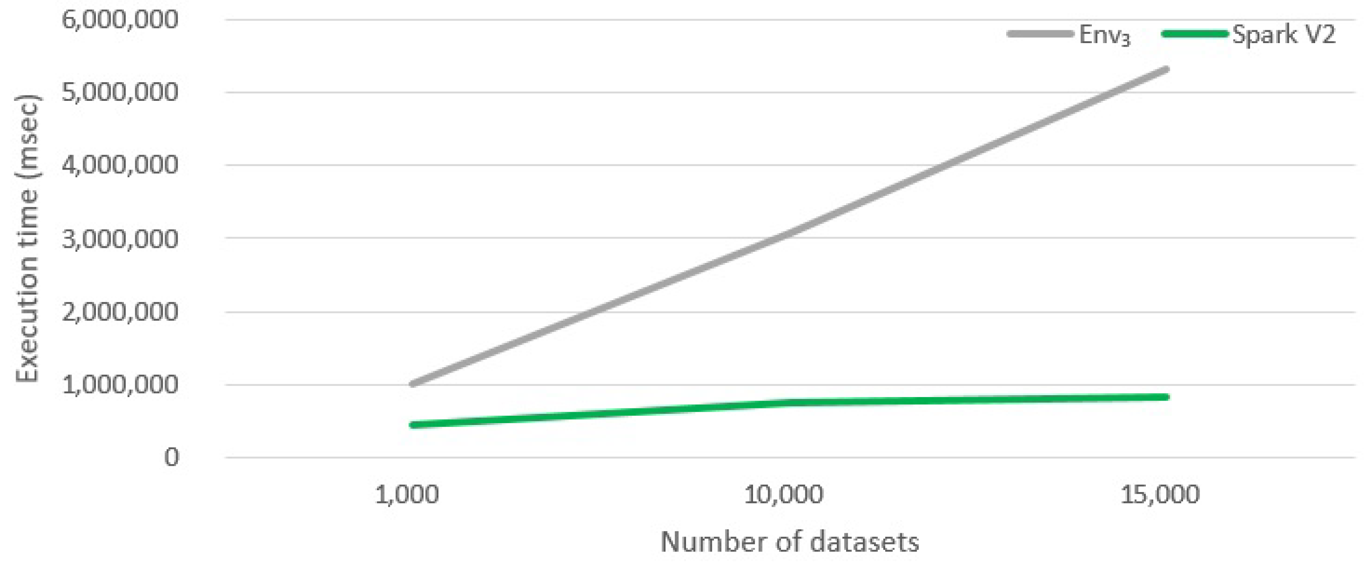
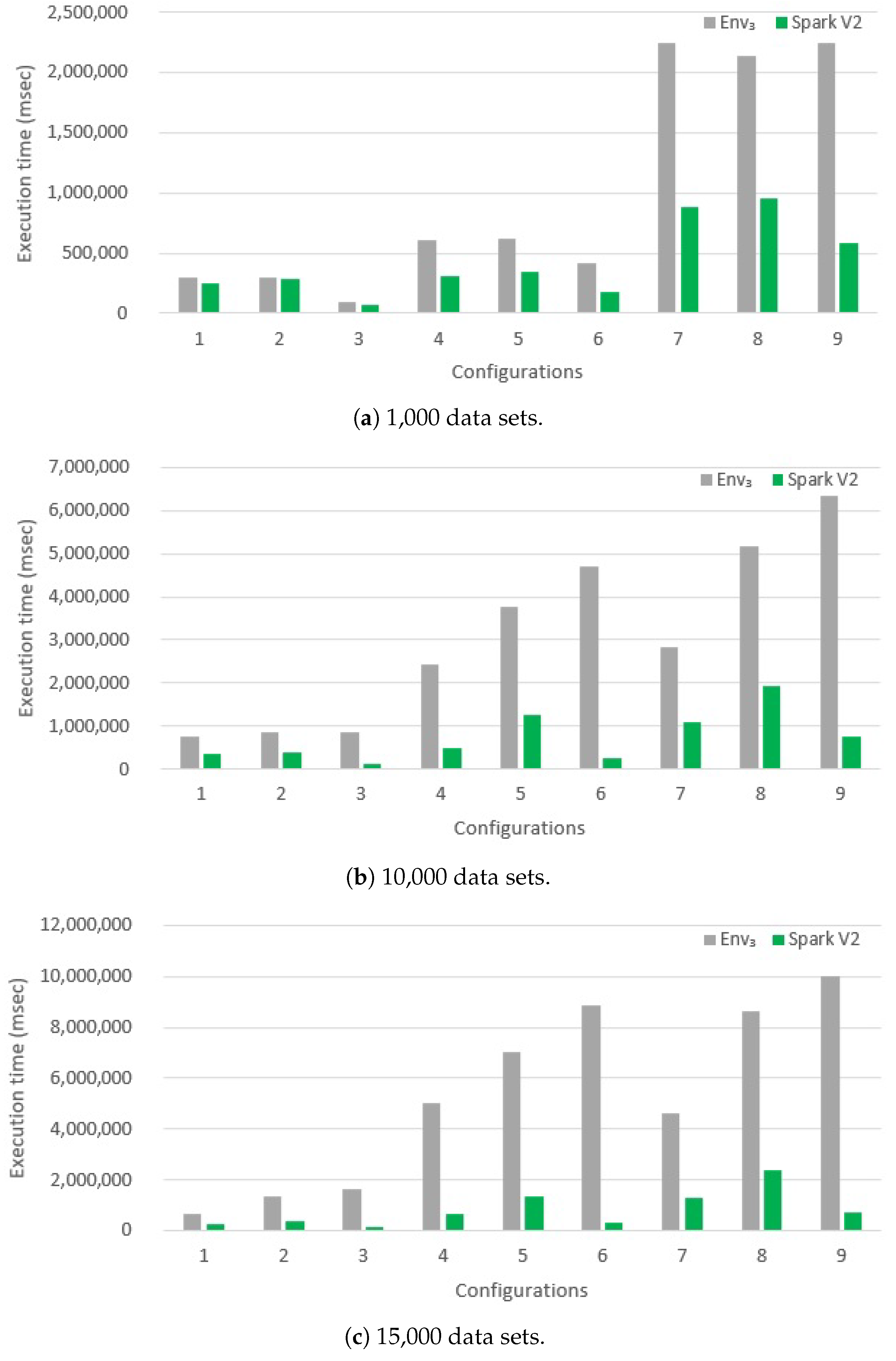
6.2.3. Evaluating Version Spark V2

The last evaluation we performed is a comparison between the Spark version of the basic Map-Reduce algorithm presented in Section 5.3 with the enhanced version presented in Section 5.4 and based on sdatasets, named Spark V2. The enhanced version was tested again in the execution environment $En{v}_3$; however, for clarity, with $En{v}_3$, we refer to results obtained with the first Spark version, while, with Spark V2 we refer to results obtained with the enhanced version.

Table 8 reports detailed execution times exhibited by version Spark V2. We compare them with execution times reported in the bottom sections of Table 5, Table 6 and Table 7.

Figure 7 compares average execution times for both the versions: notice that the average execution times of version Spark V2 are up to five times smaller than the version denoted as $En{v}_3$.

Since the hardest task is performed in Step 4, Figure 8 compares the average execution times exhibited by Step 4 only: again, version Spark V2 is much more efficient (green bars) than the previous version. In particular, notice how the gain increases when the size of the corpus increases. Observing green bars, the average execution times slightly increase, even though the size of the corpus becomes 10 times larger than the initial one.

If we deepen the analysis by evaluating configurations in detail, we can refer to

Table 11. Fraction of average execution times for version Spark V2 of the algorithm, in comparison with basic Spark implementation executed on environment $En{v}_3$.

Configurations	max_neigh	1000 Data Sets	10,000 Data Sets	15,000 Data Sets
$Con{f}_1$		82.44%	46.97%	40.74%
$Con{f}_2$	10	97.32%	44.23%	26.72%
$Con{f}_3$		78.77%	13.44%	10.58%
$Con{f}_4$		50.45%	19.71%	12.90%
$Con{f}_5$	100	56.86%	33.27%	18.80%
$Con{f}_6$		41.99%	5.63%	3.35%
$Con{f}_7$		39.37%	38.11%	28.51%
$Con{f}_8$	1000	44.41%	37.25%	27.36%
$Con{f}_9$		26.09%	12.16%	7.28%

and to Figure 9. Table 11 reports the percentage of total execution times exhibited by version Spark V2 in relation to the version denoted as $En{v}_3$ for each configuration. In some cases, version Spark V2 finishes in around 10% of the time. Looking at the table, a non-uniform behavior appears: version Spark V2 is always faster, but, in the case of configuration $Con{f}_9$ and corpus containing 15,000 data sets, the gain is less than 30%.

Figure 9 analyzes execution times exhibited by Step 4, for each single configuration and for each one of the considered corpus sizes. Notice the great improvements given by version Spark V2 of the algorithm. In particular, for configurations with 1000 queries in Q ($Con{f}_7$, $Con{f}_8$ and $Con{f}_9$), it seems that multiplying by ten the number of queries has little impact. Consequently, we can say that not only the gain is motivated by the fact that now the algorithm is decoupled from MongoDB, but also sdatasets are handled by Spark in a very efficient way.

To conclude the analysis, we observe that all the steps are improved in version Spark V2 (see Table 8), apart from Step 1: this is due to the fact that sdatasets are loaded from MongoDB in this step; the loss of performance of this step, anyway, is beneficial for the other steps.

7. Lessons We Learned and Behavioral Guidelines

The goal of this section is to summarize what we have learned from the work reported in this paper:

• Spark is a very efficient framework, due to the fact that it does not rely on the HDFS to coordinate tasks. In fact, the basic Map-Reduce version of the algorithm (presented in Section 5.3) shares a very limited amount of data among parallel tasks, i.e., query descriptors. However, since synchronization is performed always through HDFS, Hadoop is much slower than Spark.
  However, frameworks evolve: our experiment were conducted with Hadoop version 2. The new Hadoop version 3 (just released) promises to be much more efficient. Generally, Hadoop is always slower than Spark: it works with mass memory and cannot cache the data in memory, but Hadoop 3 should work up to 30% faster than the oldest version. The major difference is that version 3 provides better optimization, better and usability and a series of architectural improvements.
• Hadoop is anyway able to improve performance, if compared to the No Map-Reduce version. Anyway, developers do not have to expect incredible improvements: in our case, with n executors, the final execution time is not $1/n$, the No Map-Reduce execution time. Probably, increasing the number of nodes, we will get excellent results even with Hadoop but with a significant increase in costs.
• Spark is so effective because it coordinates parallel tasks: by building a DAG (Direct Acyclic Graph): it computes an execution plan that is shared to all nodes. In contrast, Hadoop does not offer this feature: tasks are executed in a totally non-coordinate way.
• Parallel tasks that continuously access MongoDB (and, we can expect, any other DBMS) are certainly slower than algorithms specifically designed to exploit Map-Reduce in a native way. Nevertheless, our experiments show that Spark, which is not overloaded by HDFS, performs very well, even for algorithms that are not originally designed as Map-Reduce algorithms.
• The dataset abstraction provided by Spark (that we denoted as sdataset) is extremely interesting. First of all, it allows for avoiding complex technicalities concerned with the management of the execution environment. Second, it allows developers to think at a higher level of abstraction, compared with traditional procedural programming.
• High-level abstractions provided by Spark are certainly very interesting and, in many cases, effective to reduce the development time. However, developers lose control of execution and optimization: it may happen that the level of abstractions is too high. If developers want to achieve the best performance, they probably have to scale down to low-level primitives (but, in this case, Spark programs become hard to write).
• In our context, the HDFS is not exploited for computation. However, it is a good tool to share persistent data to nodes in the cluster, especially very large data sets. Spark does not provide a similar functionality. Again, the new Hadoop version 3 could produce interesting surprises in terms of performance with large data sets.

Based on the observations reported above, we can identify some behavioral guidelines for developers that want to start developing Map-Reduce applications.

• Minimal effort. If the goal of developers is to migrate a classical algorithm to a first Map-Reduce version, by paying the minimal effort, this could be easily obtained, without changing the global structure of the algorithm. However, this can be done if the algorithm is structured as loops of complex tasks/procedures. Furthermore, connections to a DBMS can be maintained.
  We suggest adopting the Spark framework, that, in general, provides better performance, even with database connections.
• Privilege performance. If the goal of developers is to privilege performance, algorithms must be redesigned as pure Map-Reduce algorithms.
• Simplicity of design. Abstractions provided by Spark are quite effective in order to strongly simplify the design (or redesign) of an algorithm. This could be a good choice for making the development process effective and efficient.
• Hadoop or Spark? Notice that the two frameworks are not in conflict, even though the reader might think this. In fact, they can co-exist without any problem. Hadoop was created as an engine for processing large amounts of existing data: it has a low level of abstraction that allows for performing complex manipulations but can cause learning difficulties. Spark is faster, with a lot of great high-level tools and functions that can simplify the design and the development. If the algorithms or the processes do not require special features, Spark is always the most reasonable choice. However, there are situations in which the size of data is so large that the main memory of computing nodes could not be enough, causing Spark to significantly slow down. In these cases, Spark can operate on top of Hadoop and has many good libraries like Spark SQL or Spark MLlib.

8. Conclusions and Future Work

This paper reports our experience in the evolution of the Hammer query engine based on the adoption of Map-Reduce technology to improve performances. In fact, we consider this experience an interesting study case to learn about the introduction of Map-Reduce technology in algorithms that were not thought to be parallelized with this technology. Several approaches were evaluated and tested: first of all, a very simple transformation was done, tested both on top of the Hadoop framework and on top of the Spark framework. Then, a further enhanced version was developed, based on the high-level abstraction called dataset (that we called sdataset to avoid confusion) provided by Spark.

The goal of the study was to understand the impact of adopting Map-Reduce technology, learning lessons and synthesize some behavioral guidelines for developers that have to adopt Map-Reduce for the first time.

In fact, the reader can notice that our algorithms are not particularly optimized, as well as that we are working with a corpus that contains at most 15,000 data sets (thus, it is not exactly “Big Data”). Anyway, this context suffers for poor performance, due to the fact that no specific optimized data structure for representing the inverted index is adopted. Thus, we showed that the adoption of Map-Reduce does make sense.

A point we want to discuss is the generation of so many neighbor queries (up to 1000, in configurations $Con{f}_7$, $Con{f}_8$ and $Con{f}_9$): generating so many queries probably is not so useful (in [1] and, in [2], we tested the effectiveness of the technique with 10 neighbour queries, obtaining very good results); in fact, we decided to generate so many queries to stress execution times. However, four minutes to execute queries with 10 neighbor queries and 15,000 data sets (our best performance obtained with version Spark V2) is too much; thus, we are going to further study how to optimize the query engine.

Summarizing what we have learned, we can say that, currently, Spark Version 2 is, in general, more effective than Hadoop Version 2: optimization of execution, data sharing and high-level abstractions make Spark V2 a very good framework, suitable for many application contexts. However, Hadoop Version 3 has been just released and, probably, things could change.

As a future work, we are going to explore several directions. As far as efficiency, we are going to further study how to improve performance, by adopting different representations of the inverted index and by exploiting differently Spark primitives. Obviously, Hadoop Version 3 will be tested too. As far as the blind querying reconquer is concerned, we will foster its development, in order to introduce semantics to exploit during query rewriting.

References

1. Pelucchi, M.; Psaila, G.; Toccu, M.P. Building a query engine for a corpus of open data. In Proceedings of the 13th International Conference on Web Information Systems and Technologies (WEBIST 2017), Porto, Portugal, 25–27 April 2017; pp. 126–136. [Google Scholar]
2. Pelucchi, M.; Psaila, G.; Toccu, M. Enhanced Querying of Open Data Portals. In Proceedings of the International Conference on Web Information Systems and Technologies (WEBIST 2017), Porto, Portugal, 25–27 April 2017; Springer: Cham, Switzerland, 2017; pp. 179–201. [Google Scholar]
3. Pelucchi, M.; Psaila, G.; Maurizio, T. The challenge of using Map-Reduce to query open data. In Proceedings of the 6th International Conference on Data Science, Technology and Applications (DATA 2017), Madrid, Spain, 24–26 July 2017; pp. 331–342. [Google Scholar]
4. Braunschweig, K.; Eberius, J.; Thiele, M.; Lehner, W. The State of Open Data. In Proceedings of the 21st World Wide Web 2012 (WWW2012) Conference, Lyon, France, 16–20 April 2012. [Google Scholar]
5. Liu, J.; Dong, X.; Halevy, A.Y. Answering Structured Queries on Unstructured Data. In Proceedings of the WebDB 2006, Chicago, IL, USA, 30 June 2006; Volume 6, pp. 25–30. [Google Scholar]
6. Schwarte, A.; Haase, P.; Hose, K.; Schenkel, R.; Schmidt, M. FedX: A federation layer for distributed query processing on linked open data. In Proceedings of the Extended Semantic Web Conference, Heraklion, Crete, Greece, 29 May–2 June 2011; Springer: Berlin, Germany, 2011; pp. 481–486. [Google Scholar]
7. Dean, J.; Ghemawat, S. MapReduce: Simplified data processing on large clusters. Commun. ACM 2008, 51, 107–113. [Google Scholar] [CrossRef]
8. Shvachko, K.; Kuang, H.; Radia, S.; Chansler, R. The hadoop distributed file system. In Proceedings of the 2010 IEEE 26th Symposium on Mass Storage Systems and Technologies (MSST), Incline Village, NV, USA, 3–7 May 2010; pp. 1–10. [Google Scholar]
9. Bu, Y.; Howe, B.; Balazinska, M.; Ernst, M.D. HaLoop: Efficient iterative data processing on large clusters. Proc. VLDB Endow. 2010, 3, 285–296. [Google Scholar] [CrossRef]
10. Borthakur, D.; Gray, J.; Sarma, J.S.; Muthukkaruppan, K.; Spiegelberg, N.; Kuang, H.; Ranganathan, K.; Molkov, D.; Menon, A.; Rash, S.; et al. Apache Hadoop goes realtime at Facebook. In Proceedings of the 2011 ACM SIGMOD International Conference on Management of Data, Athens, Greece, 12–16 June 2011; ACM: New York, NY, USA, 2011; pp. 1071–1080. [Google Scholar]
11. Zaharia, M.; Xin, R.S.; Wendell, P.; Das, T.; Armbrust, M.; Dave, A.; Meng, X.; Rosen, J.; Venkataraman, S.; Franklin, M.J.; et al. Apache spark: A unified engine for big data processing. Commun. ACM 2016, 59, 56–65. [Google Scholar] [CrossRef]
12. Gu, L.; Li, H. Memory or time: Performance evaluation for iterative operation on hadoop and spark. In Proceedings of the 2013 IEEE 10th International Conference on High Performance Computing and Communications & 2013 IEEE International Conference on Embedded and Ubiquitous Computing (HPCC_EUC), Zhangjiajie, China, 13–15 November 2013; pp. 721–727. [Google Scholar]
13. Abadi, M.; Barham, P.; Chen, J.; Chen, Z.; Davis, A.; Dean, J.; Devin, M.; Ghemawat, S.; Irving, G.; Isard, M.; et al. Tensorflow: A system for large-scale machine learning. In Proceedings of the OSDI 2016, Savannah, GA, USA, 2–4 November 2016; Volume 16, pp. 265–283. [Google Scholar]
14. Low, Y.; Gonzalez, J.E.; Kyrola, A.; Bickson, D.; Guestrin, C.E.; Hellerstein, J. Graphlab: A new framework for parallel machine learning. arXiv, 2014; arXiv:1408.2041. [Google Scholar]
15. Burdick, D.R.; Ghoting, A.; Krishnamurthy, R.; Pednault, E.P.D.; Reinwald, B.; Sindhwani, V.; Tatikonda, S.; Tian, Y.; Vaithyanathan, S. Systems and Methods for Processing Machine Learning Algorithms in a MapReduce Environment. U.S. Patent 8,612,368, 17 December 2013. [Google Scholar]
16. Meng, X.; Bradley, J.; Yavuz, B.; Sparks, E.; Venkataraman, S.; Liu, D.; Freeman, J.; Tsai, D.; Amde, M.; Owen, S.; et al. Mllib: Machine learning in apache spark. J. Mach. Learn. Res. 2016, 17, 1235–1241. [Google Scholar]
17. Wu, X.; Zhu, X.; Wu, G.Q.; Ding, W. Data mining with big data. IEEE Trans. Knowl. Data Eng. 2014, 26, 97–107. [Google Scholar]
18. Lin, X. Mr-apriori: Association rules algorithm based on mapreduce. In Proceedings of the 2014 5th IEEE International Conference on Software Engineering and Service Science (ICSESS), Beijing, China, 27–29 June 2014; pp. 141–144. [Google Scholar]
19. Oruganti, S.; Ding, Q.; Tabrizi, N. Exploring Hadoop as a platform for distributed association rule mining. In Proceedings of the Fifth International Conference on Future Computational Technologies and Applications (FUTURE COMPUTING 2013), Valencia, Spain, 27 May–1 June 2013; pp. 62–67. [Google Scholar]
20. Chang, L.; Wang, Z.; Ma, T.; Jian, L.; Ma, L.; Goldshuv, A.; Lonergan, L.; Cohen, J.; Welton, C.; Sherry, G.; et al. HAWQ: A massively parallel processing SQL engine in hadoop. In Proceedings of the 2014 ACM SIGMOD International Conference On Management of Data, Snowbird, UT, USA, 22–27 June 2014; ACM: New York, NY, USA, 2014; pp. 1223–1234. [Google Scholar]
21. Chung, W.C.; Lin, H.P.; Chen, S.C.; Jiang, M.F.; Chung, Y.C. JackHare: A framework for SQL to NoSQL translation using MapReduce. Autom. Softw. Eng. 2014, 21, 489–508. [Google Scholar] [CrossRef]
22. Kononenko, O.; Baysal, O.; Holmes, R.; Godfrey, M. Mining Modern Repositories with Elasticsearch. In Proceedings of the 11th Working Conference on Mining Software Repositories (MSR), Hyderabad, India, 29–30 June 2014. [Google Scholar]
23. Shahi, D. Apache Solr: An Introduction. In Apache Solr; Springer: Berlin, Germany, 2015; pp. 1–9. [Google Scholar]
24. Croft, W.B.; Metzler, D.; Strohman, T. Search Engines: Information Retrieval in Practice; Addison-Wesley Reading: Boston, NA, USA, 2010; Volume 283. [Google Scholar]
25. Manning, C.D.; Raghavan, P.; Schütze, H. Introduction to Information Retrieval; Cambridge University Press: Cambridge, UK, 2008; Volume 1. [Google Scholar]
26. Winkler, W.E. The State of Record Linkage and Current Research Problems; Statistical Research Division, U.S. Census Bureau: Washington, DC, USA, 1999.
27. White, T. Hadoop: The Definitive Guide; O’Reilly Media, Inc.: Sebastopol, CA, USA, 2012. [Google Scholar]
28. Borthakur, D. The hadoop distributed file system: Architecture and design. Hadoop Proj. Website 2007, 11, 21. [Google Scholar]
29. Vavilapalli, V.K.; Murthy, A.C.; Douglas, C.; Agarwal, S.; Konar, M.; Evans, R.; Graves, T.; Lowe, J.; Shah, H.; Seth, S.; et al. Apache hadoop yarn: Yet another resource negotiator. In Proceedings of the 4th annual Symposium on Cloud Computing, Santa Clara, CA, USA, 1–3 October 2013; ACM: New York, NY, USA, 2013; p. 5. [Google Scholar]
30. Ekanayake, J.; Li, H.; Zhang, B.; Gunarathne, T.; Bae, S.H.; Qiu, J.; Fox, G. Twister: A runtime for iterative mapreduce. In Proceedings of the 19th ACM International Symposium on High Performance Distributed Computing, Chicago, IL, USA, 21–25 June 2010; ACM: New York, NY, USA, 2010; pp. 810–818. [Google Scholar]
31. Zhang, Y.; Gao, Q.; Gao, L.; Wang, C. Imapreduce: A distributed computing framework for iterative computation. J. Grid Comput. 2012, 10, 47–68. [Google Scholar] [CrossRef]
32. Zaharia, M.; Chowdhury, M.; Franklin, M.J.; Shenker, S.; Stoica, I. Spark: Cluster computing with working sets. HotCloud 2010, 10, 95. [Google Scholar]
Figure 1. Blind querying scenario.
Algorithms 11 00209 g001
Figure 2. General architecture of the Hammer prototype.
Algorithms 11 00209 g002
Figure 3. General architecture of the Query Engine.
Algorithms 11 00209 g003
Figure 4. Average execution times.
Algorithms 11 00209 g004
Figure 5. Average execution times for Step 4.
Algorithms 11 00209 g005
Figure 6. Comparing execution times of Step 4 for each configuration, among the three different execution environments for the basic Map-Reduce algorithm.
Algorithms 11 00209 g006
Figure 7. Comparing average execution times of the basic Spark implementation (denoted as E n v 3 ) and the enhanced Spark implementation (denoted as Spark V2).
Algorithms 11 00209 g007
Figure 8. Comparing average execution times of of Step 4 for the basic Spark implementation (denoted as E n v 3 ) and the enhanced Spark implementation (denoted as Spark V2).
Algorithms 11 00209 g008
Figure 9. Comparing execution times of Step 4 for each configuration, between the basic Spark version ( E n v 3 ) and the enhanced Spark version (Spark V2).
Algorithms 11 00209 g009