Weak Fault Detection of Tapered Rolling Bearing Based on Penalty Regularization Approach

Abstract

Aimed at the issue of estimating the fault component from a noisy observation, a novel detection approach based on augmented Huber non-convex penalty regularization (AHNPR) is proposed. The core objectives of the proposed method are that (1) it estimates non-zero singular values (i.e., fault component) accurately and (2) it maintains the convexity of the proposed objective cost function (OCF) by restricting the parameters of the non-convex regularization. Specifically, the AHNPR model is expressed as the L1-norm minus a generalized Huber function, which avoids the underestimation weakness of the L1-norm regularization. Furthermore, the convexity of the proposed OCF is proved via the non-diagonal characteristic of the matrix B^TB, meanwhile, the non-zero singular values of the OCF is solved by the forward–backward splitting (FBS) algorithm. Last, the proposed method is validated by the simulated signal and vibration signals of tapered bearing. The results demonstrate that the proposed approach can identify weak fault information from the raw vibration signal under severe background noise, that the non-convex penalty regularization can induce sparsity of the singular values more effectively than the typical convex penalty (e.g., L1-norm fused lasso optimization (LFLO) method), and that the issue of underestimating sparse coefficients can be improved.

1. Introduction

Condition maintenance and health management (CMHM) of rotating machines are of great significance to prevent machinery breakdown and increase system reliability in modern industrial applications [1,2,3]. Vibration signals processing represents the most commonly used technique for monitoring the condition of rotating machines. However, in practice, such vibration signals are often contaminated and submerged by severe background noises and other interfering components, which results in a very low detection accuracy. Therefore, to accurately extract the useful weak information from the measured vibration signal becomes a hotspot issue in the area of mechanical fault diagnosis.

A number of state-of-the-art methodologies including wavelet/wavelet packet transform (W-WPT) [4,5], adaptive signal decomposition (ASD) [6,7,8] and high-order cyclic spectral analysis (HOCS) [9,10], have been developed for detecting weak fault information of rotating machinery under strong noise. Recently, sparse low-rank matrix regularization (SLMR) methods, that estimate the fault signal through solving optimization problems (or inverse problems), have attracted significant attention because of their ability to induce sparsity of the fault signal (or singular values) more effectively than the traditional sparse over-complete dictionaries (SODs) such as step-impulse dictionary and unit-impulse response dictionary [11,12,13,14,15]. For the SLMR, in particular, we consider the problem of estimating fault signal x from the acquired signal y, i.e., y = Ax + w, where signal w represents additive noise. To estimate the fault signal x, the optimization problem can be expressed by minimizing the objective cost function (OCF) F(x), i.e., $\hat{x}==\arg \underset{x}{\min }\{\frac{1}{2}{\Vert y-\mathit{A}x\Vert }_2^2+\lambda \theta (x)\},\lambda >0$, where $\theta (x)$ is a penalty function that induces sparsity of the approximating value of x and λ is the regularization term parameter.

Methodologies for SLMR can be roughly categorized as convex and non-convex penalty regularization approaches. Among convex penalty functions, L1-norm penalty function is commonly used to regularize linear inverse problems, i.e., penalty function $\theta (x)={\Vert x\Vert }_1$. In that case, the OCF F(x) is trivially convex and the global optimum can be obtained. Unfortunately, the L1-norm may underestimate the sparse coefficients of the underlying signal [16,17]. In contrast, numerous non-convex penalties (e.g., L_P pseudo-norm with p < 1 [18], reweighted L2/L1 norm [19]) and non-convex algorithms (e.g., orthogonal matching pursuit, OMP) have been proposed [20,21,22,23,24,25], which estimate non-zero components more accurately than convex regularization. However, the previous non-convex penalties were considered based on separable penalty functions and thus suffer from several issues such as sensitivity to changes with initial data and regularization term parameters, etc., and the convexity of the OCF cannot be guaranteed simultaneously. Therefore, the core objective of SLMR is to determine how to maintain convexity of the OCF when the regularizer (or penalty function) is taken to be non-convex, so that the fault component can be estimated accurately from its noisy observation.

To address such issues, a novel non-separable non-convex regularizer, namely augmented Huber penalty function, is developed in this paper, which overcomes limitations of separable non-convex regularization and ensures the strict convexity of the OCF. Specifically, the augmented penalty function is firstly defined by L1-norm and generalized Huber functions, the strict convexity and convexity condition of the proposed OCF is then derived and provided. Meanwhile, an iterative algorithm (e.g., forward–backward splitting, FBS) is presented as a solution to the proposed objective cost function. Lastly, both the simulated signal and engineering bearing data of larger reducers are employed to validate the effectiveness of the proposed approach in terms of diagnostic accuracy and signal-to-noise ratio, etc.

The layout of this work is organized as follows: Section 2 introduces the algorithm and theoretical derivation of the augmented penalty optimization; Section 3 presents the simulation evaluation of the proposed augmented Huber non-convex penalty regularization (AHNPR) method; In Section 4, the practical diagnosis results and discussion for tapered bearing using the proposed approach with other methods are presented; and Conclusions are drawn in Section 5.

2. Augmented Huber Non-Convex Penalty Regularization

2.1. Sparse Representation

Generally, estimating a sparse component x from its noisy observation y can be expressed as

$$y=\mathit{A}x+w$$

(1)

where w is the additive noise. It should be noted that Equation (1) belongs to a highly underdetermined equation, i.e., ill-posed or non-deterministic polynomial-time hard (N-P hard) problem [26], and there are an infinite set of solutions. Convex and non-convex optimization approaches are commonly used to estimate a sparse component from its noisy signal. A suitable optimization problem for estimating x is

$$\hat{x}=\arg \underset{x}{\min }\{\frac{1}{2}{\Vert y-\mathit{A}x\Vert }_2^2+\lambda {\Vert \mathit{D}x\Vert }_1\}$$

(2)

where λ is regularization term parameter and $\mathit{D}=\left[\begin{array}{llll}-1,1& & & \\ & \dots & & \\ & & \dots & \\ & & & -1,1\end{array}\right],\mathit{D}\in {ℝ}^{(N-1)\times N}$, which controls the sparsity of the approximating value of x. The above problem is well-known as the L1-norm minimization, and the L1-norm is used as a convex function for sparsity. If the signal x is a sparse component, i.e., most of the amplitude values in x tend to zero, then the problem in Equation (1) can be solved by L1-norm fused lasso optimization (LFLO) algorithm, i.e.,

$$\hat{x}=\arg \min \{\frac{1}{2}{\Vert y-\mathit{A}x\Vert }_2^2+{\lambda }_0{\Vert x\Vert }_1+{\lambda }_1{\Vert \mathit{D}x\Vert }_1\}$$

(3)

where λ₀ and λ₁ are regularization parameters. The solution of the LFLO algorithm can be given by a soft-threshold function [27], i.e.,

$$x=\mathrm{Soft}(\mathrm{tvd}(y,{\lambda }_1),{\lambda }_0)$$

(4)

where $\mathrm{tvd}(\cdot ,\cdot )$ is the total variation de-noising (TVD) model [28,29,30] and the soft-threshold function is defined as follows:

$$\mathrm{Soft}(x,\lambda )=\{\begin{array}{cc}x+\lambda ,& x<-\lambda \hfill \\ 0,& -\lambda \le x\le \lambda \hfill \\ x-\lambda ,& x>\lambda \hfill \end{array}$$

(5)

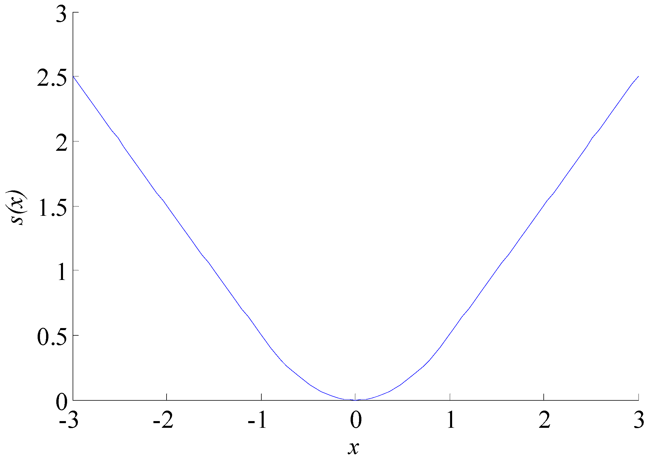
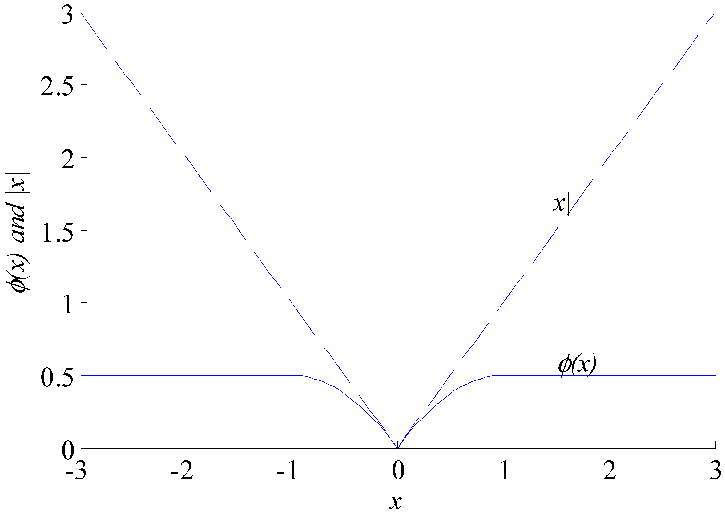
2.2. The Augmented Huber Non-Convex Penalty Regularization

In this section, before the elicitation of the proposed AHNPR algorithm, the following definitions and proposition for convex analysis should be reviewed first.

The Huber equation is defined through two piecewise functions [31,32], i.e.,

$$s(x)=\{\begin{array}{ll}\frac{1}{2}{x}^2,& \left|x\right|\le 1\\ \Vert x\Vert -\frac{1}{2},& \left|x\right|\ge 1\end{array}$$

(6)

The plot of Huber function s(x) is illustrated in Figure 1.

Let b denote a scale and the scaled Huber function (SHF) can be defined as

$$s_b(x)=\frac{1}{b^2}s(b^{2}x),b\ne 0$$

(7)

For b = 0, i.e., $s_0(x)=0$. For b ≠ 0, the scaled Huber function is given by

$$s_b(x)=\{\begin{array}{ll}\frac{1}{2}{b}^2{x}^2,& \left|x\right|\le 1/b^2\\ \left|x\right|-\frac{1}{2b^2},& \left|x\right|\ge 1/b^2\end{array}$$

(8)

Note that $0\le s_b(x)\le \left|x\right|,\forall x\in R$, i.e., $\underset{b\to \infty }{\lim }{s}_b(x)=\left|x\right|$ and $\underset{b\to 0}{\lim }{s}_b(x)=0$.

For the definition of SHF, the SHF could be rewritten through a minimization form, i.e.,

$$s_b(x)=\underset{v\in ℝ}{\min }\left\{{\Vert v\Vert }_1+\frac{1}{2}{b}^2{(x-v)}^2\right\}$$

(9)

Proof 1.

According to the SHF, i.e., $s_b(x)=\frac{1}{b^2}s(b^{2}x),b\ne 0$, Equation (9) can be rewritten as

$$\begin{array}{l}{s}_b(x)=\underset{v\in ℝ}{\min }\left\{{\Vert v\Vert }_1+\frac{1}{2}{(b^{2}x-v)}^2\right\}/b^2\\ =\underset{v\in ℝ}{\min }\left\{{\Vert b^{2}v\Vert }_1+\frac{1}{2}{(b^{2}x-b^{2}v)}^2\right\}/b^2\\ =\underset{v\in ℝ}{\min }\left\{{\Vert v\Vert }_1+\frac{1}{2}{b}^2{(x-v)}^2\right\}\end{array}$$

(10)

Let B denote a matrix and the generalized Huber function (GHF) can be defined as

$$s_B(x)=\underset{v\in ℝ}{\min }\left\{{\Vert v\Vert }_1+\frac{1}{2}{\Vert \mathit{B}(x-v)\Vert }_2^2\right\}$$

(11)

In summary, if matrix B evolves into a scale, i.e., B = b, then the GHF reduces to the SHF, $s_B(x)=s_b(x)$ for all x.

If B is a matrix and B^TB = I is a diagonal, then the GHF is separable, and $s_B(x)$ is the sum of the SHF $s_b(x)$, i.e., ${\mathit{B}}^T\mathit{B}=\mathrm{Diag}(b_1,b_2,\cdots ,b_N)\Rightarrow s_B(x)={\displaystyle \sum _N{s}_{b_n}(x_n)}$. In contrast, if B^TB ≠ I is a non-diagonal matrix, the GHF is non-separable.

Based on the definitions above, the new non-separable non-convex penalty function can be derived using the GHFs. The new non-separable non-convex penalty (NNP) function $\varphi (x)$ is defined as

$$\varphi (x)=\{\begin{array}{ll}\left|x\right|-\frac{1}{2}{x}^2,& \left|x\right|\le 1\\ \frac{1}{2},& \left|x\right|\ge 1\end{array}$$

(12)

Therefore, according to the definition of Huber function, the function $\varphi (x)$ can be expressed as

$$\varphi (x)=\left|x\right|-s(x)$$

(13)

where s(x) is the Huber function. Similarly, the plot of NNP function $\varphi (x)$ is illustrated in Figure 2.

Let b denote a scale of function and the scaled NNP function can be defined as

$${\varphi }_b(x)=\left|x\right|-s_b(x)$$

(14)

where $s_b(x)$ is SHF. For b = 0, i.e., ${\varphi }_0(x)=\left|x\right|$. For b ≠ 0, the scaled NNP function is given by

$${\varphi }_b(x)=\{\begin{array}{ll}\left|x\right|-\frac{1}{2}{b}^2{x}^2,& \left|x\right|\le 1/b^2\\ \frac{1}{2b^2},& \left|x\right|\ge 1/b^2\end{array}$$

(15)

Let B denote a matrix and the NNP function $\varphi (x)$ will evolve into an augmented Huber function (AHF) ${\varphi }_B(x)$, i.e.,

$${\varphi }_B(x)={\Vert x\Vert }_1-s_B(x)$$

(16)

where $s_B(x)$ is the generalized Huber function (GHF).

Given a matrix B, if B^TB = 0, then ${\varphi }_B(x)={\Vert x\Vert }_1$; if B^TB = I is a diagonal matrix, then AHF ${\varphi }_B(x)$ is separable, and ${\varphi }_B(x)$ is the sum of the scaled NNP function $s_b(x)$, i.e., ${\mathit{B}}^T\mathit{B}=\mathrm{Diag}(b_1^2,b_2^2,\cdots ,b_N^2)\Rightarrow {\varphi }_B(x)={\displaystyle \sum _N{\varphi }_{b_n}(x_n)}$. If ${\mathit{B}}^T\mathit{B}=\mathrm{Diag}(b_1^2,b_2^2,\cdots ,b_N^2)$, then we have

$$\begin{array}{l}{\varphi }_B(x)={\Vert x\Vert }_1-{\displaystyle \sum _N{s}_{b_n}(x_n)}\\ ={\displaystyle \sum _N{\left|x\right|}_n-s_{b_n}(x_n)}\\ ={\displaystyle \sum _N{\varphi }_{b_n}(x_n)}\end{array}$$

(17)

In contrast, if B^TB is a non-diagonal matrix, the AHF ${\varphi }_B(x)$ is non-separable.

Thus, the proposed AHNPR method finds the component x by solving the following optimization problem:

$$\begin{array}{l}F(x)=\frac{1}{2}{\Vert y-\mathit{A}x\Vert }_2^2+\lambda {\varphi }_B(x)\\ =\frac{1}{2}{\Vert y-\mathit{A}x\Vert }_2^2+\lambda [{\Vert x\Vert }_1-S_B(x)]\end{array}$$

(18)

where F(x) is the objective cost function (OCF), and ${\varphi }_B(x)$ is the AHF, which is a non-convex sparsity inducing regularizer.

2.3. Convexity Condition

In this section, the convexity of the proposed OCF will be proved to consider how to set the parameter τ and the relationship between matrix A and matrix B.

If $y\in {ℝ}^M$, $\mathit{A}\in {ℝ}^{M\times N}$ is a matrix, the regularization term parameter λ > 0 and the proposed OCF $F(x)=\frac{1}{2}{\Vert y-\mathit{A}x\Vert }_2^2+\lambda {\varphi }_B(x)$ is convex, then the matrix B^TB satisfies

$${\mathit{B}}^T\mathit{B}\le \frac{1}{\lambda }{\mathit{A}}^T\mathit{A}$$

(19)

Proof 2.

According to $s_B(x)=\underset{v\in ℝ}{\min }\left\{{\Vert v\Vert }_1+\frac{1}{2}{\Vert \mathit{B}(x-v)\Vert }_2^2\right\}$ and ${\varphi }_B(x)={\Vert x\Vert }_1-s_B(x)$, the F(x) can be rewritten as

$$\begin{array}{l}F(x)=\frac{1}{2}{\Vert y-\mathit{A}x\Vert }_2^2+\lambda [{\Vert x\Vert }_1-s_B(x)]\\ =\frac{1}{2}{\Vert y-\mathit{A}x\Vert }_2^2+\lambda {\Vert x\Vert }_1-\underset{v\in ℝ}{\min }\left\{\lambda {\Vert v\Vert }_1+\frac{\lambda }{2}{\Vert \mathit{B}(x-v)\Vert }_2^2\right\}\\ =\underset{v\in ℝ}{\max }\left\{\frac{1}{2}{\Vert y-\mathit{A}x\Vert }_2^2+\lambda {\Vert x\Vert }_1-\lambda {\Vert v\Vert }_1-\frac{\lambda }{2}{\Vert \mathit{B}(x-v)\Vert }_2^2\right\}\\ =\underset{v\in ℝ}{\max }\left\{\frac{1}{2}{x}^T({\mathit{A}}^T\mathit{A}-\lambda {\mathit{B}}^T\mathit{B})x+\lambda {\Vert x\Vert }_1+g(x,v)\right\}\\ =\frac{1}{2}{x}^T({\mathit{A}}^T\mathit{A}-\lambda {\mathit{B}}^T\mathit{B})x+\lambda {\Vert x\Vert }_1+\underset{v\in ℝ}{\max }g(x,v)\end{array}$$

(20)

where A^T is the complex conjugate transpose of matrix A, and B^T is the complex conjugate transpose of matrix B. The last term $\underset{v\in ℝ}{\max }g(x,v)$ is convex due to the point-wise maximum of a set of convex functions [31]. Hence, the proposed OCF F(x) is convex if it satisfies ${\mathit{A}}^T\mathit{A}-\lambda {\mathit{B}}^T\mathit{B}\ge 0$.

For convexity condition ${\mathit{B}}^T\mathit{B}\le \frac{1}{\lambda }{\mathit{A}}^T\mathit{A}$, it can be rewritten as ${\mathit{B}}^T\mathit{B}=(\tau /\lambda ){\mathit{A}}^T\mathit{A}$, in which the parameter τ satisfies τ ≤ 1. Hence, given a matrix A, the matrix B could be set as $\mathit{B}=\sqrt{\tau /\lambda }\mathit{A},0\le \tau \le 1$. The parameter τ controls the non-convexity of the AHF ${\varphi }_B(x)$. If τ = 0, then B = 0 and function ${\varphi }_B(x)$ reduces to the L1-norm. If τ = 1, then ${\mathit{B}}^T\mathit{B}=(\tau /\lambda ){\mathit{A}}^T\mathit{A}$ and the function ${\varphi }_B(x)$ are maximally non-convex.

Here, the nominal range of parameter τ is discussed by a simulated discrete signal. Given a simulated systematic signal of

$$\begin{array}{l}f(t)=f_1(t)+\mathrm{Noise}\\ =M_0\sin (2\pi f_{1}t)+M_1\cos (2\pi f_{2}t)+\mathrm{Noise}\end{array}$$

(21)

where the amplitudes of M₀ and M₁ are 1 and 2, respectively, the signal length is N = 100 with the frequencies f₁ = 0.25 and f₂ = 0.4. For the de-noising experiment, the Gaussian noise with σ = 1.5 is added to acquire the simulated systematic signal. The systematic signal f(t) is approximately sparse in the frequency domain, as illustrated in Figure 3, which can be represented by f = Ax, where A is an over-sampled inverse discrete Fourier transform and x is a sparse vector of Fourier coefficients. Specifically, matrix A is defined as ${\mathit{A}}_{m,n}=(1/\sqrt{N})\exp (j(2\pi /N)mn)$, $m=0,1,\cdots ,M-1;n=0,1,\cdots ,N-1$, with M = 100 and N = 256. Assuming that matrix A^T is the complex conjugate transpose of matrix A and it can be calculated that B^TB is a diagonal matrix.

In order to obtain a nominal range of parameter $0\le \tau \le 1$, we vary the parameter τ from 0.05 to 0.95 (by increments of 0.05) and calculate each root-mean-square error (RMSE) between the actual value $f_1(t)$ and its estimated value $\widehat{f_1(t)}$, and also we calculate the optimized coefficients (or Fourier coefficients amplitude) at frequencies f₁ = 0.25 and f₂ = 0.4 for each parameter τ. The RMSE values and optimized coefficients for each parameter τ are shown in Figure 4. From Figure 4a, it can be seen that the larger value of parameter τ would get a lower value of RMSE, and the optimal parameters τ are concentrated in the $0.8\le \tau \le 0.9$ range. As a matter of fact, the smaller value of parameters τ would make the estimated signal noisier and less sparse. From Figure 4b, it is found that the optimized coefficients at f₁ = 0.25 increase and then slightly decrease with increasing parameter τ; meanwhile, the optimized coefficients at f₁ = 0.4 increase as parameter τ increases. From the point of view that the significant coefficients are not underestimated and get a clearer signal $f_1(t)$, the optimal parameters τ are also concentrated in the $0.8\le \tau \le 0.9$ range. Therefore, in practice the nominal range of parameter τ is set to $0.8\le \tau \le 0.9$.

For the selection of the regularization parameter λ, we have

$$\lambda =\gamma \times {\beta }_0\times \sigma$$

(22)

where σ is the standard deviation (SD) of the additive noise, ${\beta }_0$ is the constant so as to maximize the signal-to-noise ratio (SNR). Here, parameters β₀ and γ are typically set to be constant values, i.e., β₀ = [0.5, 1], γ = [7.5, 8]. In practice, the standard deviation (SD) of the background noise in Equation (22) can be computed using the fault signal and healthy data under the same operating environment. Moreover, when the healthy data are not available or are unknown, the standard deviation (SD) of background noise can still be estimated by the following formula:

$$\hat{\sigma }=MAD(y)/0.6745$$

(23)

which is a traditional estimator of the noise level used for wavelet de-noising [33], where MAD(y) represents the median absolute deviation (MAD) of signal y, i.e.,

$$MAD(y)=\mathrm{median}(\left|y_i-\mathrm{median}(y)\right|),i=1,2,\dots ,N$$

(24)

As an example, if we take the constant parameters to be β₀ = 0.7 and γ = 7.5, with the regularization parameter λ = 7.5 × 0.7 × 1.5 = 7.875, the solutions of LFLO and proposed AHNPR method with parameter τ = 0.8 are shown in Figure 5. Comparing the results of the LFLO and proposed AHNPR methods, the proposed AHNPR solution is sparser than the results of LFLO in frequency domain (see Figure 5c) and the LFLO underestimates significant coefficients of the underlying signal.

Therefore, in practice, based on the above analysis, the optimal parameter τ is set to be $0.8\le \tau \le 0.9$, the constant parameters β₀ and γ are set to be β₀ = 0.7 and γ = 7.5, and the regularization parameter λ is set to be $\lambda =\gamma \times {\beta }_0\times \sigma$.

Finally, in order to minimize the F(x), and assuming ${\mathit{B}}^T\mathit{B}=(\tau /\lambda ){\mathit{A}}^T\mathit{A}$ with parameter 0.8 ≤ τ ≤ 0.9, the optimization problem could be transformed into saddle-point problem, i.e.,

$$\begin{array}{l}(x^{opt},v^{opt})=\arg \underset{x\in ℝ}{\min }\underset{v\in ℝ}{\max }F(x,v)\\ =\arg \underset{x\in ℝ}{\min }\underset{v\in ℝ}{\max }\left\{\frac{1}{2}{\Vert y-\mathit{A}x\Vert }_2^2+\lambda {\Vert x\Vert }_1-\lambda {\Vert v\Vert }_1-\frac{\lambda }{2}{\Vert \mathit{B}(x-v)\Vert }_2^2\right\}\end{array}$$

(25)

The solution of the saddle-point problem can be obtained using the forward–backward splitting (FBS) algorithm, [34], as listed in Algorithm 1.

Algorithm 1 Iterative algorithm for the proposed AHNPR method

Initialization: $x^{(0)}$,$v^{(0)}$, $0<\mu <2/\max \{1,\tau /(1-\tau )\}\cdot {\Vert A^{T}A\Vert }_2$;

For $i=0,1,2,\dots$; $w^{(i)}=x^{(i)}-\mu A^T\{A[x^{(i)}+\tau (v^{(i)}-x^{(i)})]-y\}$

$u^{(i)}=v^{(i)}+\mu \tau A^{T}A(x^{(i)}-v^{(i)})$

$x^{(i+1)}=\mathrm{soft}(w^{(i)},\lambda \mu )$

$v^{(i+1)}=\mathrm{soft}(u^{(i)},\lambda \mu )$

end return: $x^{(i+1)}=\mathrm{soft}(w^{(i)},\lambda \mu )$

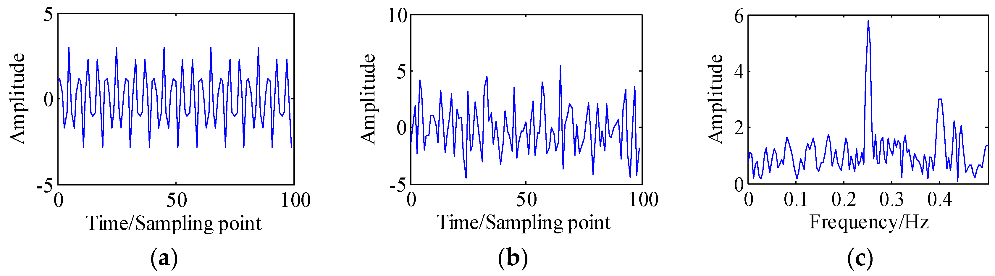
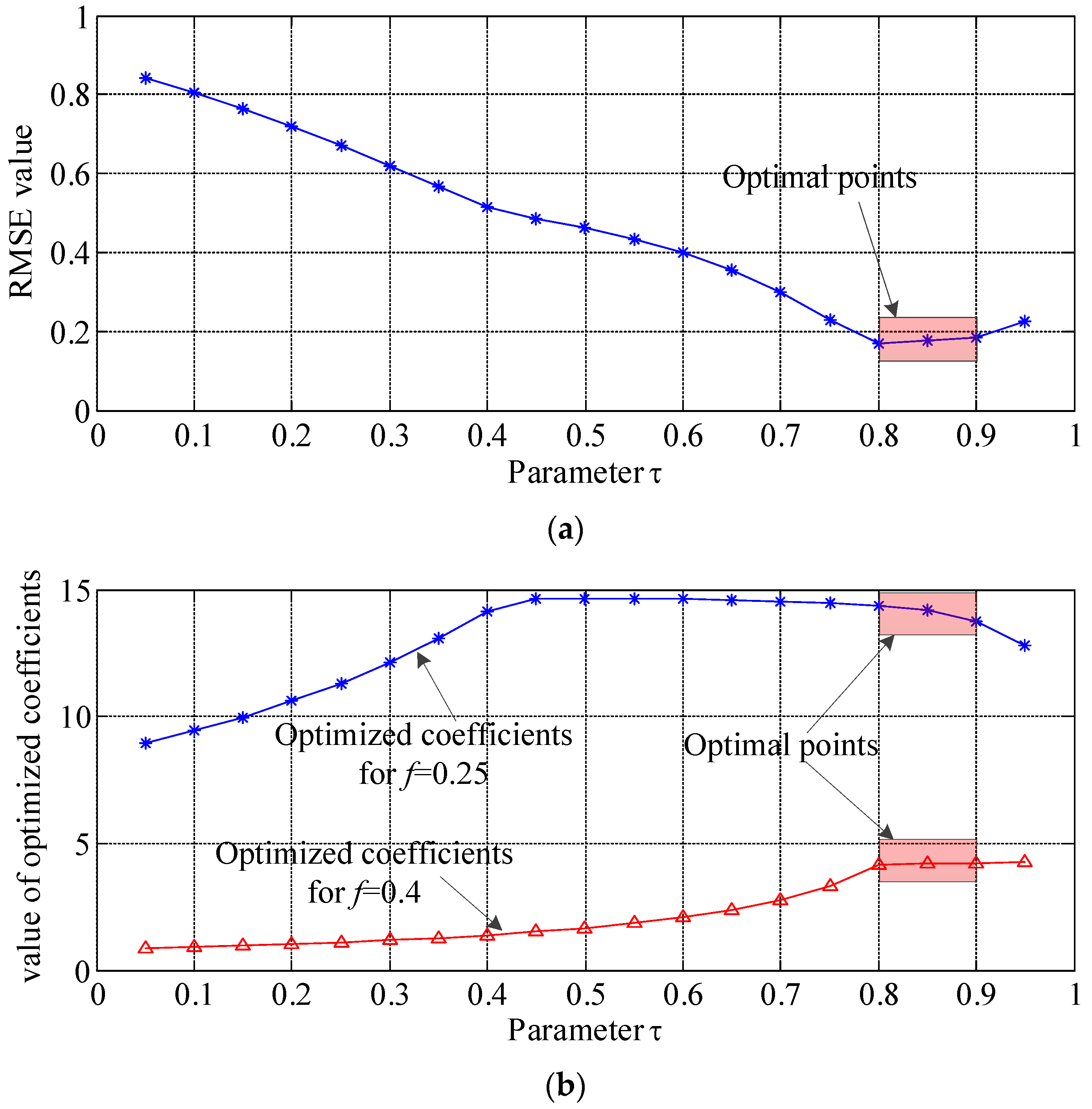
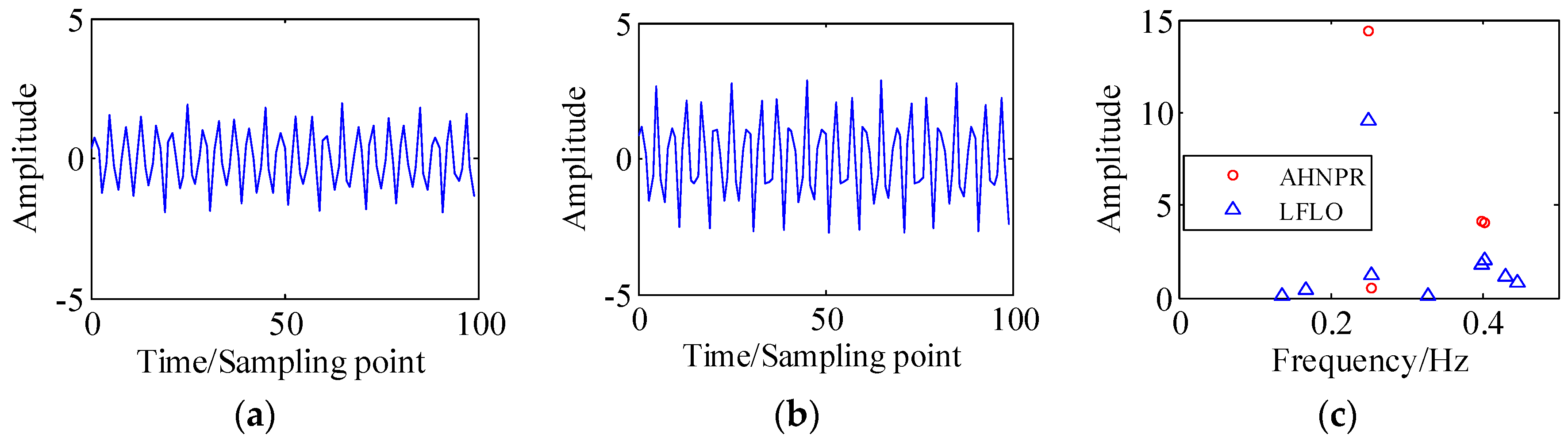
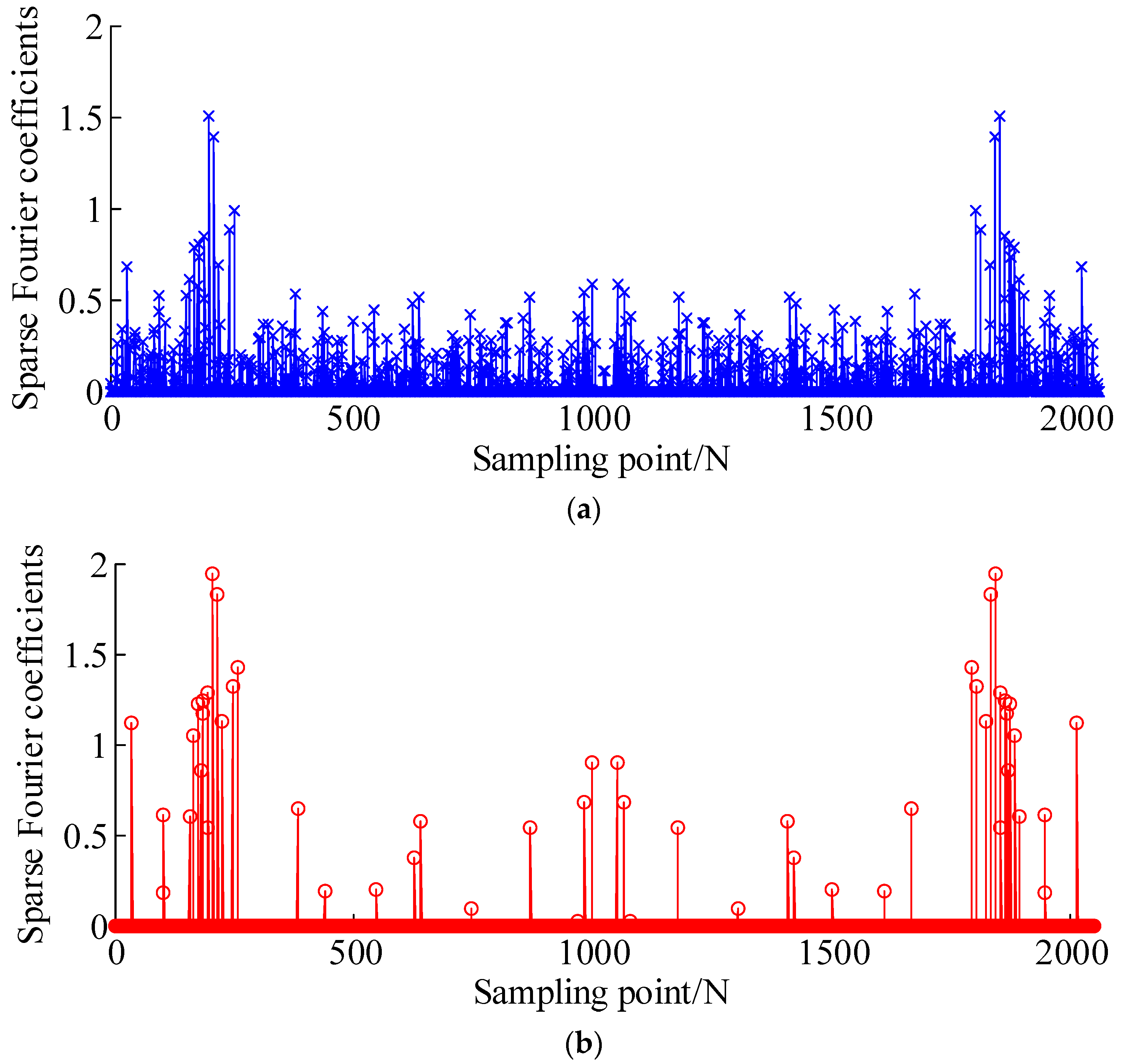
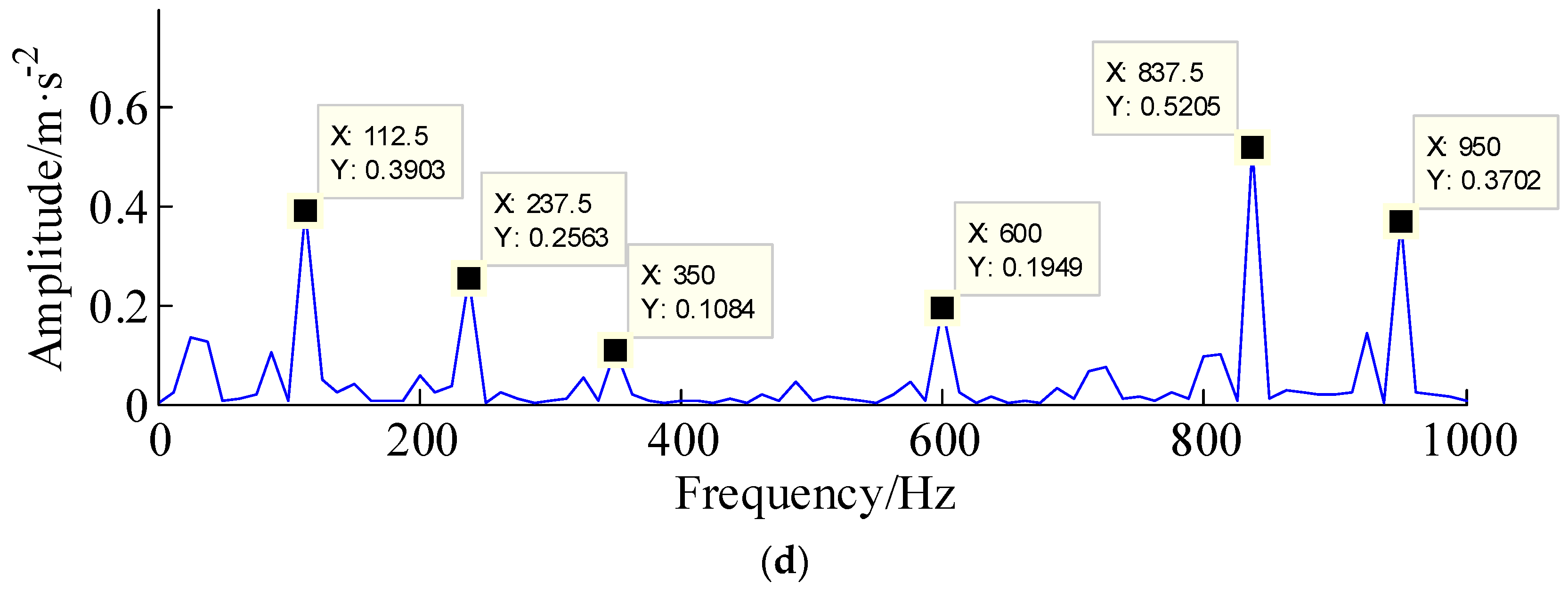
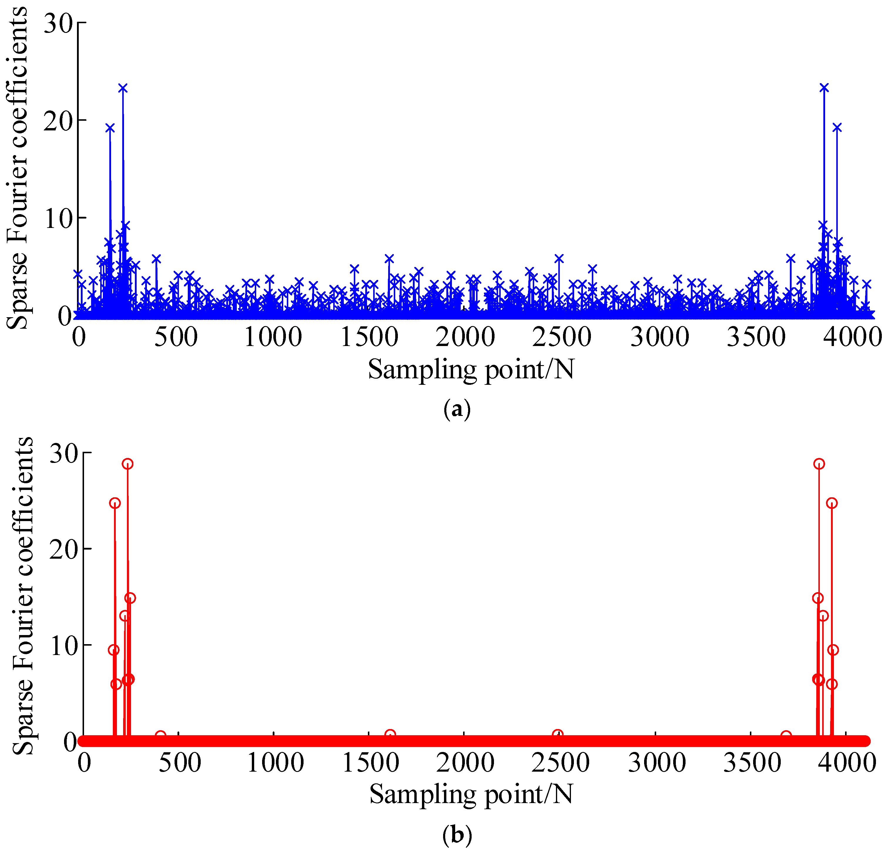
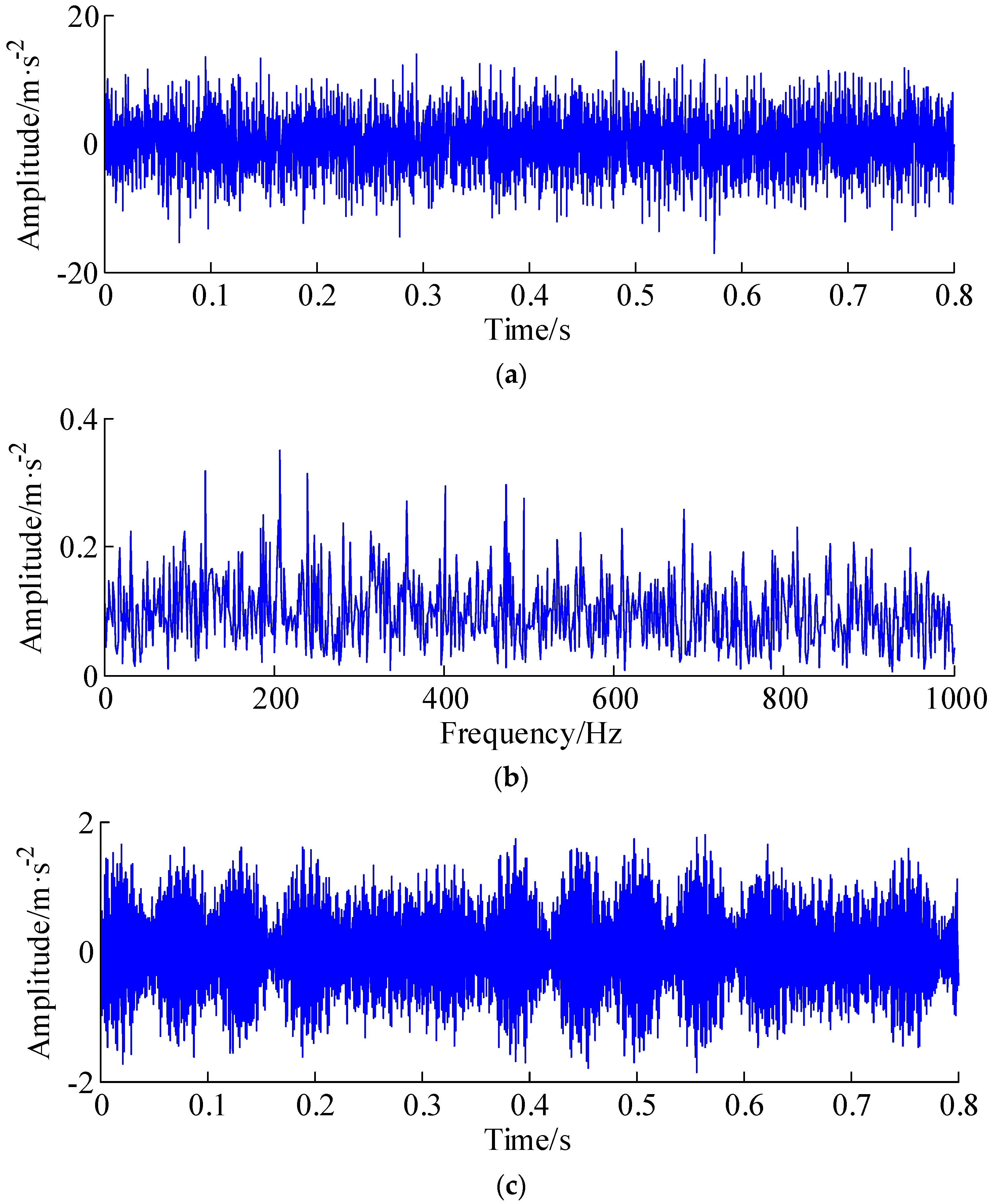
3. Numerical Simulation

A simulation signal is utilized to investigate the effectiveness of the proposed AHNPR approach. Considering the periodical impulse features that are generated by the localized fault in rotating machinery, the simulation signal is constructed as

$$\begin{array}{l}y(t)=x(t)+\mathrm{Noise}\\ =\exp (-a\times 2\pi f_{n}t)\times \sin (2\pi f_n\times \sqrt{1-a^2}t)+\sigma \times \mathrm{randn}(1,N)\end{array}$$

(26)

where a = 0.1 is a damping coefficient, the structural frequency of system is f_n = 2000 Hz, signal length is N = 2048, and the sampling frequency is f_s = 20 KHz. In addition, the additive Gaussian noise with σ = 0.4 is added to acquire the simulated synthetic signal. Figure 6a,c depict the obtained periodical impulses with localized faults and the simulated synthetic signal. Figure 6b,d are the corresponding Morlet wavelet time-frequency diagrams of periodical impulses and simulated synthetic signals, respectively. From Figure 6c,d, it is seen that the periodic impulses are completely buried in heavy background noise.

Following this, the proposed AHNPR method is applied to process the simulated synthetic signal. Specifically, matrix A is defined as ${\mathit{A}}_{m,n}=(1/\sqrt{N})\exp (j(2\pi /N)mn)$; here, $m=0,1,\cdots ,M-1;n=0,1,\cdots ,N-1$. Assuming that matrix A^T is the complex conjugate transpose of matrix A, it can be calculated that A^TA is a diagonal matrix, the parameter τ is set to τ = 0.8, and thus matrix B is $B=\sqrt{\tau /\lambda }A$. In addition, taking the constant parameters to be β₀ = 0.7 and γ = 7.5, the parameter λ could be calculated by Equation (22), i.e., λ = 7.5 × 0.7 × 0.4 = 2.1. Since B^TB is a non-diagonal matrix, the augmented Huber penalty function ${\varphi }_B(x)$ is non-separable.

The de-noising results of the LFLO method and proposed AHNPR method are shown in Figure 7a,c, respectively. Figure 7b,d are the corresponding Morlet wavelet time-frequency diagrams of Figure 7a,c, respectively. It can be noted that the periodic characteristics in Figure 7c are more obvious than in Figure 7a. The sparse Fourier coefficients of LFLO and the proposed AHNPR method are shown in Figure 8a,b. The non-convex penalty function method aims to induce sparsity in sparse coefficients more effectively than the LFLO method. Moreover, the LFLO method underestimates the significant (large-amplitude) sparse coefficients of the de-noised signal.

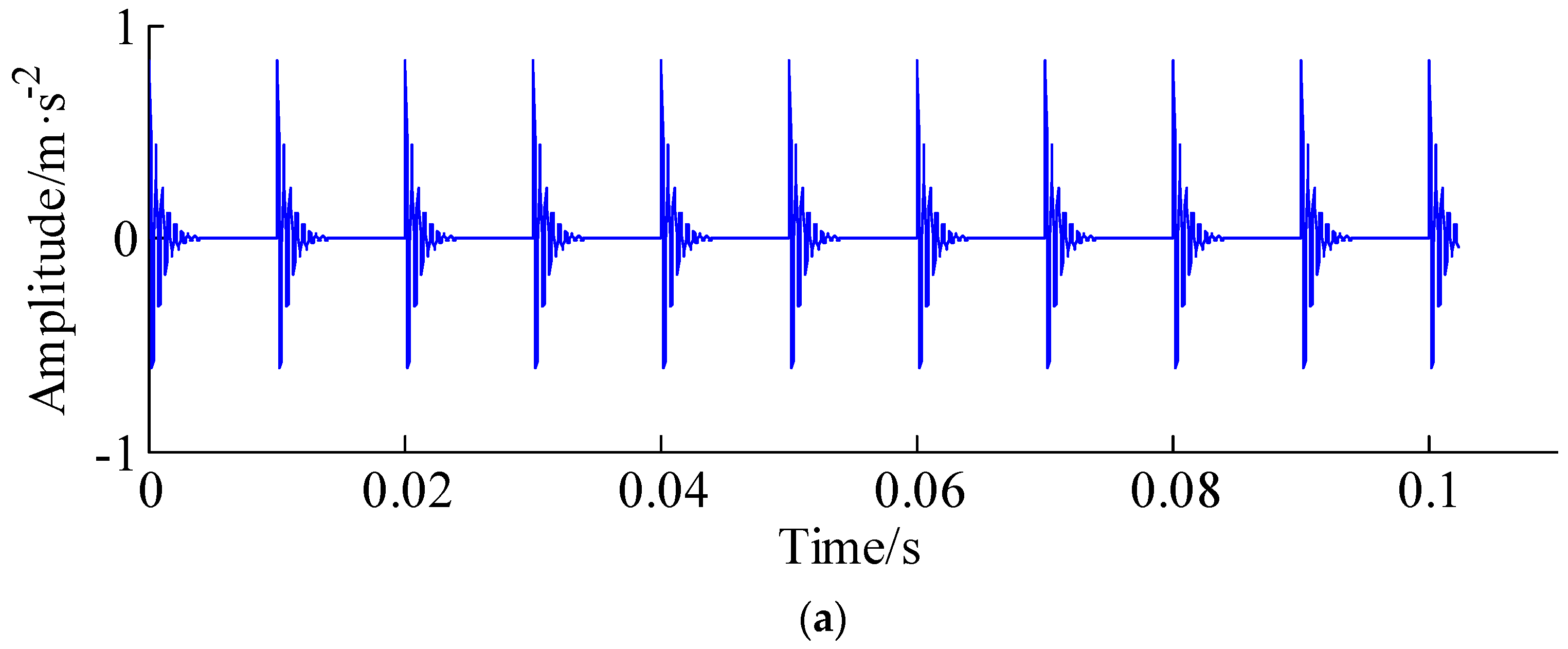
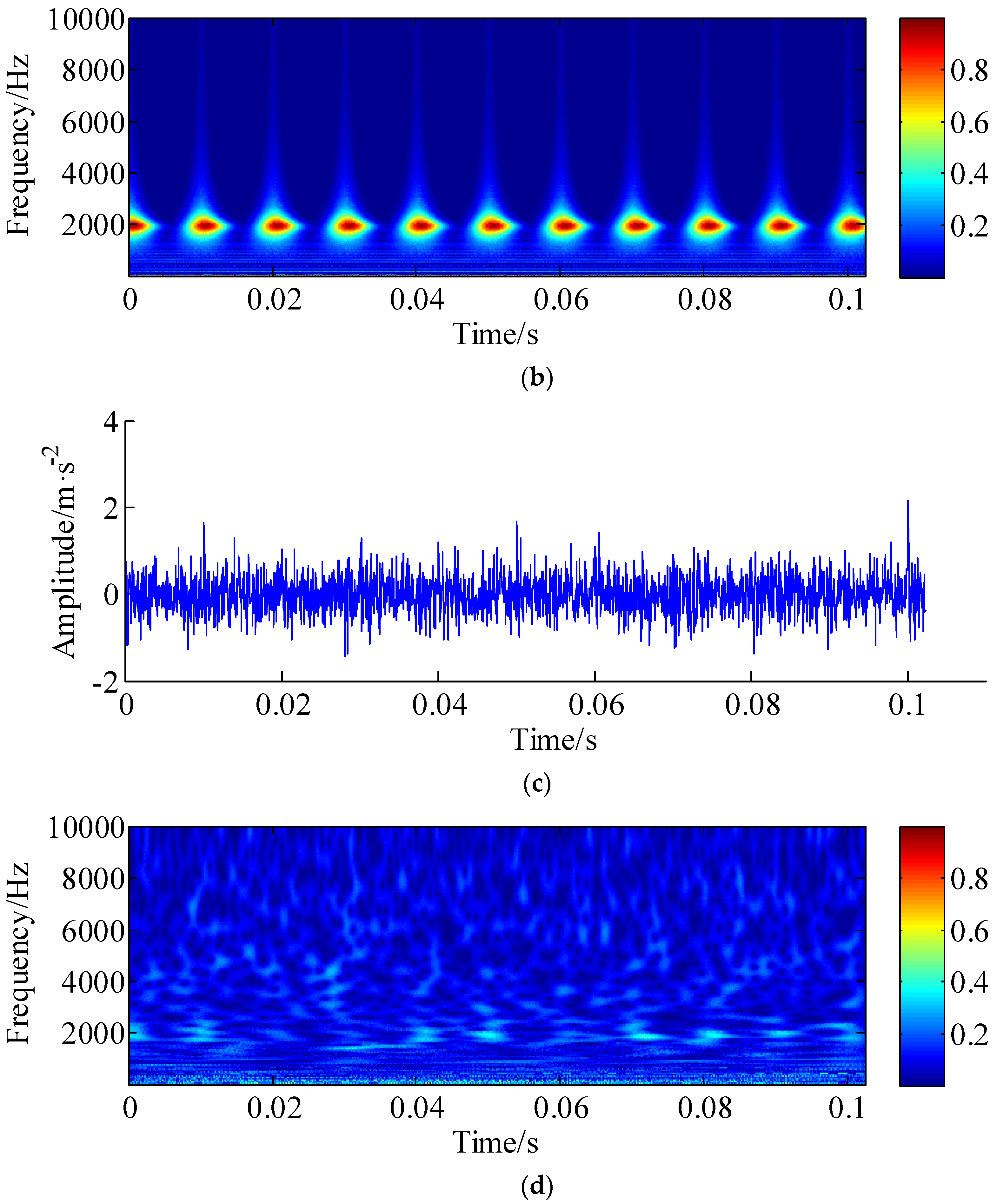
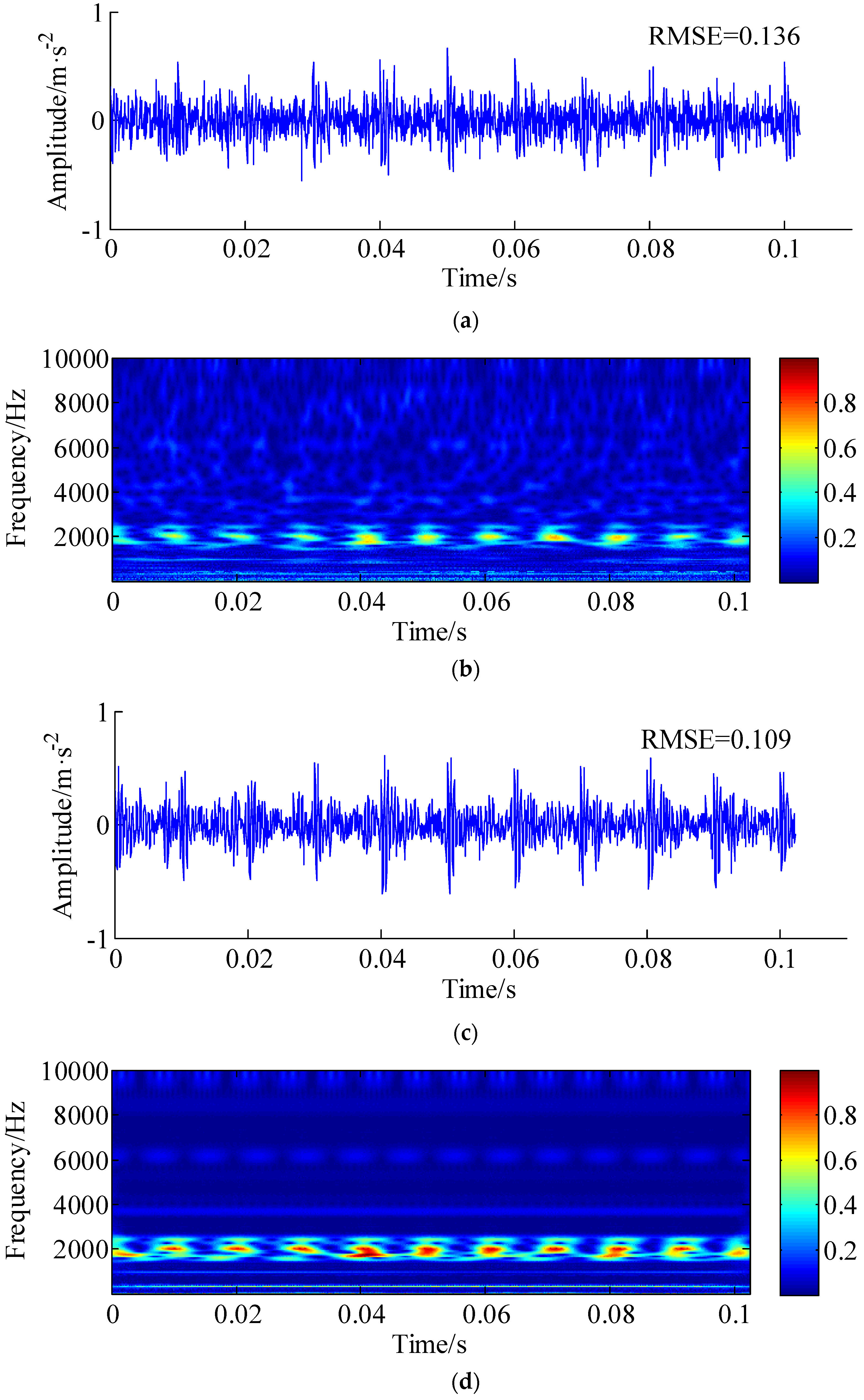
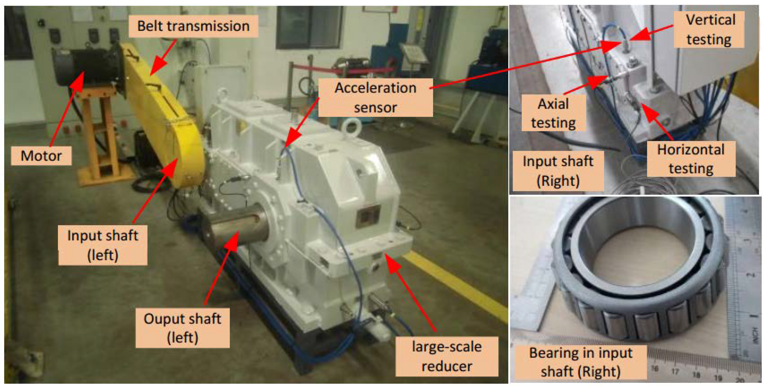
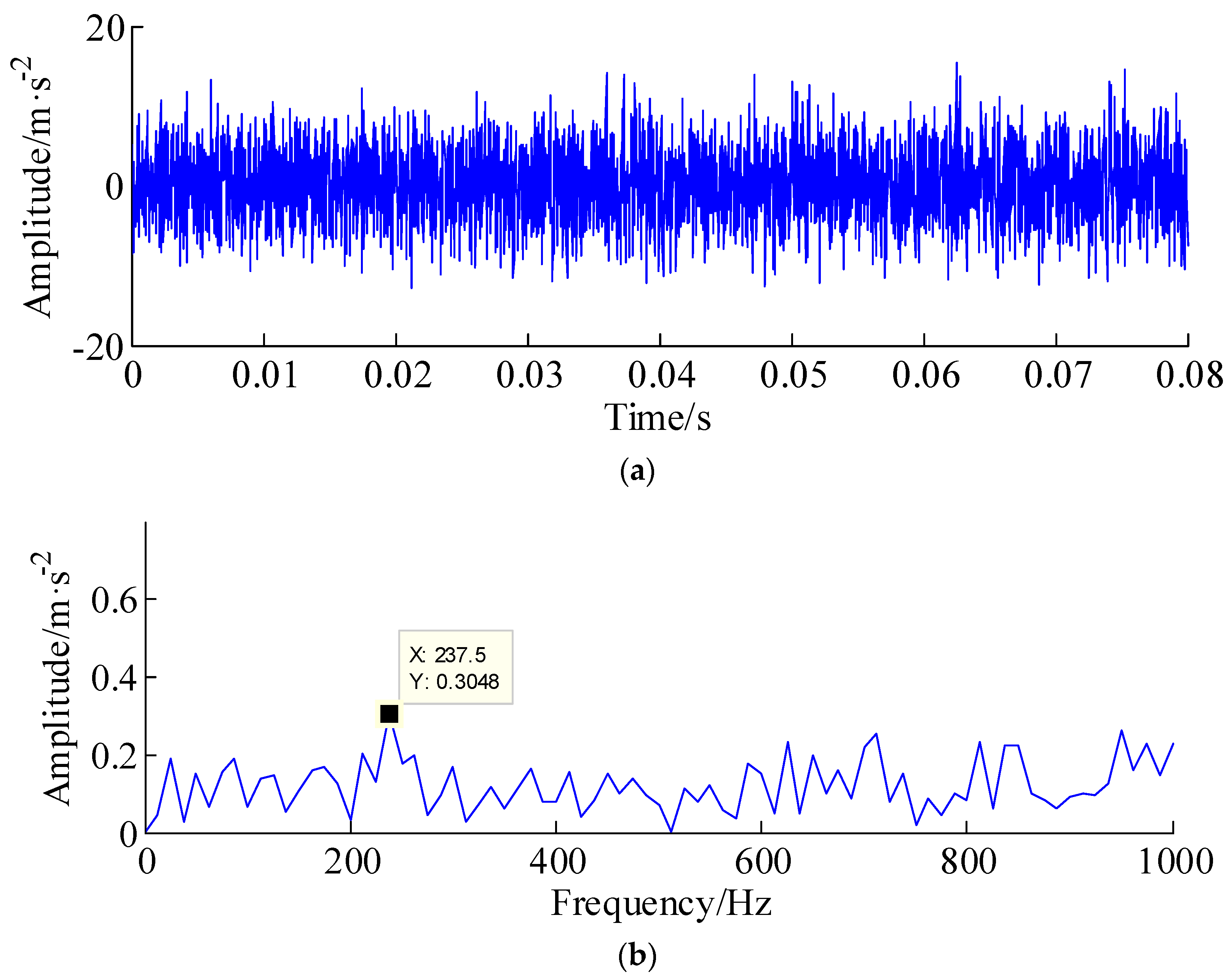
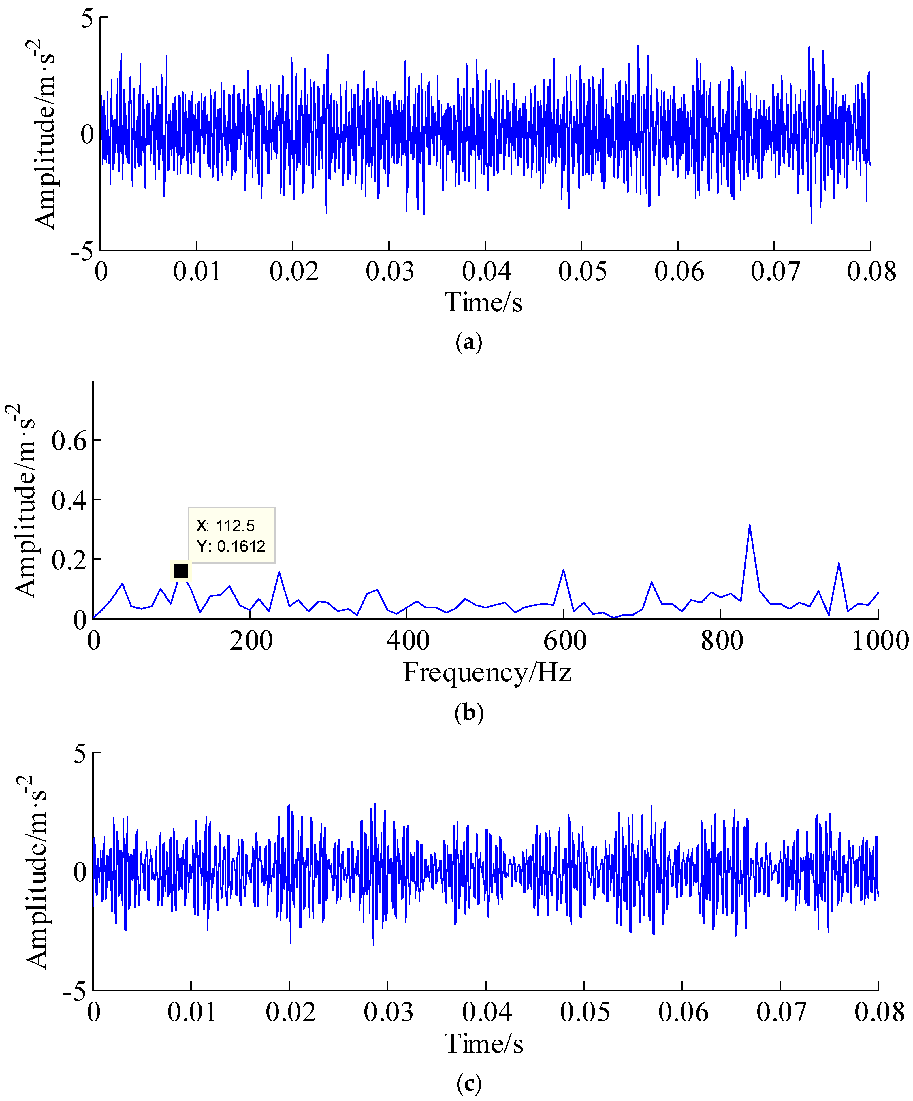
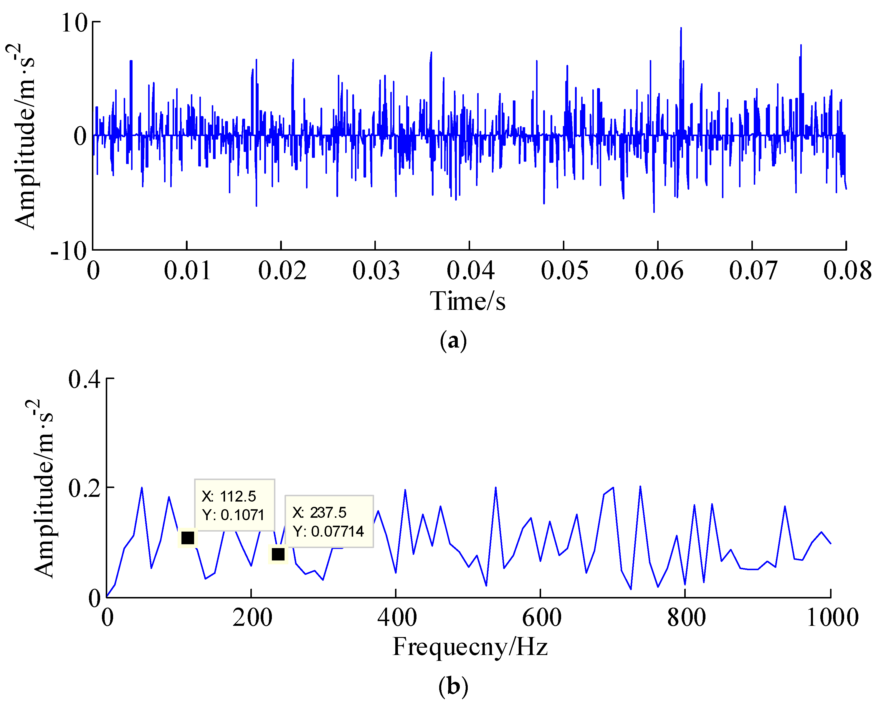
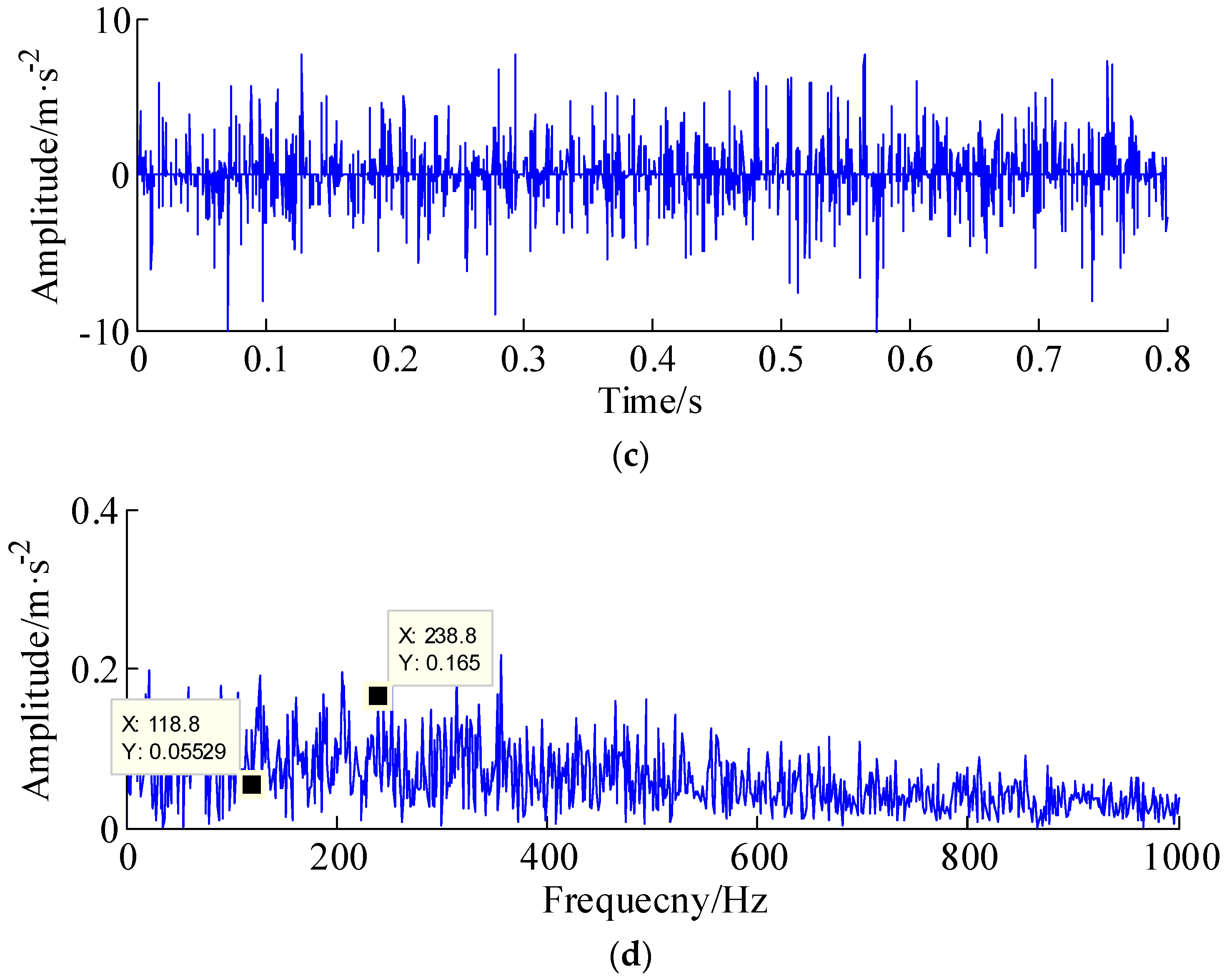
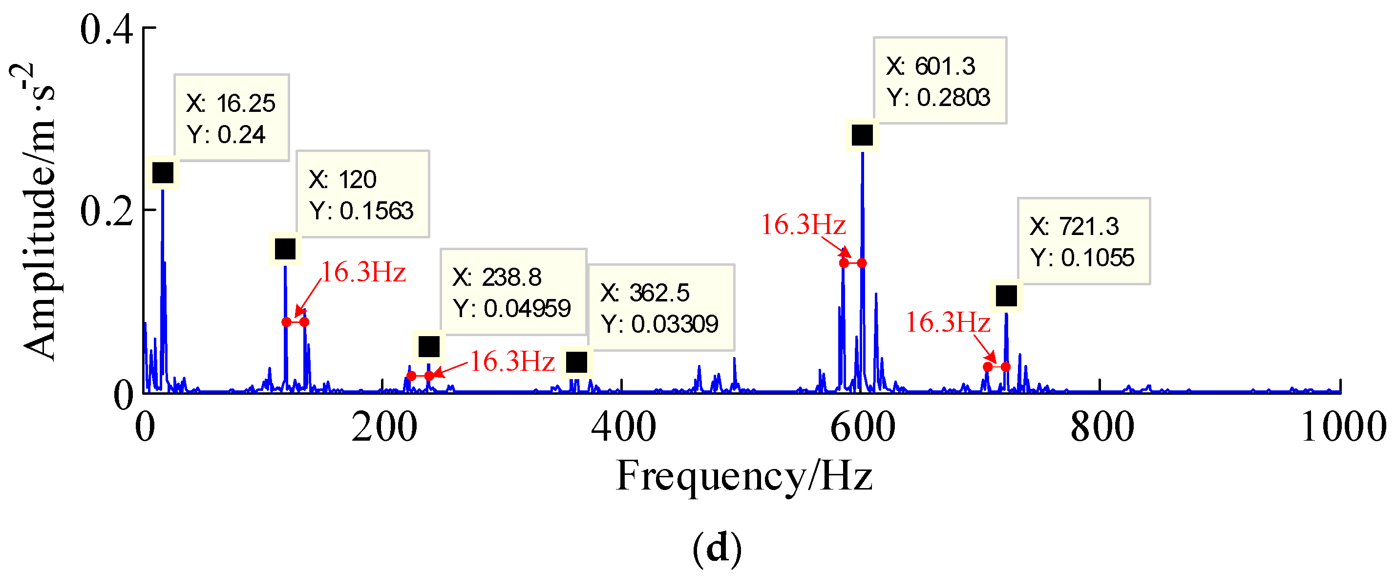
4. Experimental Verification

To demonstrate the validity of the proposed approach in engineering applications, the tapered rolling bearing with a faulty outer race is implemented. Experimental vibration data were collected from several accelerometers instrumented on a bearing end bracket from a large reducer, as shown in Figure 9. The geometrical parameters of the tested tapered bearing are listed in

Table 1. The geometrical parameters of the tested tapered rolling bearing.

Bearing Type	Fault Type	Number of Balls	Inner Diameter	Outer Diameter	Fault Frequency
FAG-32212-A	Outer race	9	60 mm	110 mm	118.8 Hz

, and the fault frequency of the bearing outer race is 118.8 Hz. The sampling frequency is 51.2 KHz (right side of input shaft) and 5.12 KHz (left side of input shaft), the rotation frequency is 16.67 Hz and sampling length is 6.4 s. The tapered rolling bearing (FAG-32212-A) fault was located on the right side of the input shaft. In this experiment, the vibration data collected from the right side of input shaft (horizontal direction, i.e., non-drive end) were used in the first experiment. To create a more challenging condition, the vibration data collected from the left side of the input shaft (horizontal direction, drive end) were also analyzed in the second experiment.

The first experiment had two tasks, i.e., to estimate the weak fault signal from the original vibration signal and to calculate the sparsity of the sparse coefficient. The raw vibration signal (right side of input shaft, 4096 sampling points were selected, i.e., 0.08 s) and its envelop spectrum are displayed in Figure 10a,b, respectively. As shown in Figure 10b, although the spectrum peak at 237.5 Hz, which is consistent with the twice outer-race fault frequency, can be detected; however, the spectrum peak is masked by heavy background noise and frequency features are not clear enough to detect practical fault.

The proposed AHNPR approach and the LFLO method are respectively employed to process the measured vibration signal and the obtained results are displayed in Figure 11. The parameter $\tau$ was set to τ = 0.8 and matrix A is also defined as ${\mathit{A}}_{m,n}=(1/\sqrt{N})\exp (j(2\pi /N)mn),m=0,1,\cdots ,M-1;n=0,1,\cdots ,N-1$. Thus, matrix B is $\mathit{B}=\sqrt{0.8/\lambda }\mathit{A}$. It can be calculated that B^TB is a non-diagonal matrix, thus the augmented Huber function (AHF) ${\varphi }_B(x)$ is non-separable. Here, it should be noted that the healthy data are not available or are unknown, according to Equations (23) and (24). Taking the constant parameters to be β₀ = 0.7 and γ = 7.5, the parameters of the proposed method can be obtained as follows: the standard deviation σ = 4.234, and regularization term parameters λ = 7.5 × 0.7 × 4.234 = 22.23. Comparing results with the time-domain waveform and envelope spectrum, one can observe improvements at two levels: the first is the significant enhancement in the contribution of periodical characteristic. The periodical characteristic with LFLO is weaker than that related to the proposed method. The second improvement is that the amplitudes of fault frequency and its harmonic are worthy of further enhancement. Note that some other unrelated components in Figure 11d are greatly reduced compared with the envelope spectra of the raw signal and the de-noised signal generated by the LFLO method.

In addition, the distribution of sparse coefficients generated by LFLO and the proposed AHNPR method are given in Figure 12a,b, respectively. One can see that the sparse coefficients are underestimated by the LFLO method along with the sparse coefficients associated with additive noise that reduce sparsity. In comparison with the LFLO result, the sparse coefficients of the proposed AHNPR method are enhanced and amplified.

As to the second experiment, Figure 13a,b present the raw vibration signal on the drive end (i.e., the left side of the input shaft, 4096 sampling points were selected, i.e., 0.8 s) and its envelope spectrum. In this case, the outer race fault frequency cannot be observed. This may be caused by the fact that the outer race fault is quite weak and the transfer path of the accelerometers located on the left side are longer than in the previous experiment. As such, the proposed AHNPR algorithm is applied to separate the fault feature from other unrelated components and the results are displayed in Figure 13c,d. The parameters of the proposed method can be obtained as follows: the standard deviation σ = 4.44, regularization term parameter λ = 7.5 × 0.7 × 4.4 = 23.31, and parameter τ is set to τ = 0.8.

The outer race fault frequency and its harmonics are detected in the corresponding envelope spectrum. In addition, interestingly, the sidebands are distributed in both fault frequency and its harmonics, after calculating the difference between the fault frequencies and sidebands. It should be noted that the difference values are consistent with the rotational frequency (16.67 Hz). Therefore, the outer race fault of bearings can be more clearly diagnosed. The above result demonstrates that the proposed algorithm can detect the bearing fault and eliminate the background noise interference, regardless of whether the accelerometers are located on the right or left side of the input shaft.

In previous research [35], another non-convex penalty regularization approach, namely the asymmetric convex penalty regularization (ACPR) method, was proposed for weak fault detection for gearboxes. To explore the advantage of the proposed approach over the ACPR method, the diagnosis results under same operation environments are compared, the ACPR method is introduced to process the same data that collected from the right side and left side of the input shaft, respectively, and the rules of parameter settings are based on the reference [35]. The sparse component of right-side of input shaft generated by the ACPR method is shown in Figure 14a, and its envelop spectrum is shown in Figure 14b. Likewise, the sparse component of left-side of input shaft generated by the ACPR method is presented in Figure 14c, and its envelop spectrum is presented in Figure 14d. From the time-domain waveform of Figure 14a,b, the separating effect generated by the ACPR method is better than the results that generated by proposed method, and the noise components are decimated drastically, but the fault frequency of the bearing outer race and its harmonic cannot be extracted using the ACPR method, as shown in Figure 14b,d. This is because the ACPR algorithm contains two penalty functions, i.e., symmetric and asymmetric penalty functions, here the asymmetric function is established using simple quadratic polynomial, which may not be appropriate for such data. Compared with the traditional envelop spectrum method, the LFLO method and the ACPR method, the final comparative results show the effectiveness and superiority of the proposed diagnosis method.

5. Conclusions

This paper proposes a novel weak fault detection approach for tapered rolling bearing based on the augmented Huber nonconvex penalty regularization (AHNPR) approach. The purpose of this paper is to overcome the following two problems: (1) The traditional convex regularizer (e.g., L1-norm) may underestimate sparse coefficients of the underlying signal; and (2) the convexity of the objective function cannot be guaranteed using traditional separable non-convex penalties regularizers.

In this work, we proposed an AHNPR for solving the low-rank matrix approximation (LRMA) problem (or inverse problem). Compared to the LFLO algorithm, where the singular values would be calculated by a soft-threshold function, the proposed method does not underestimate singular values. The AHNPR is known to estimate singular values more accurately. In addition, an efficient algorithm using the forward–backward splitting (FBS) technique to solve the proposed OCF is derived. Finally, the effectiveness of the proposed method is demonstrated by the simulated vibration signal practical rolling bearing under severe additive background noise.

A possible future direction of research involves the use of AHFs, which are focused on multi-fault diagnosis under variable speed or variable harsh running environments.

References

1. Lin, J.S.; Dou, C.H. A novel method for condition monitoring of rotating machinery based on statistical linguistic analysis and weighted similarity measures. J. Sound Vib. 2017, 390, 272–288. [Google Scholar] [CrossRef]
2. Li, Q.; Liang, S.Y. Degradation trend prognostics for rolling bearing using improved R/S statistic model and fractional Brownian motion approach. IEEE Access 2018, 6, 21103–21114. [Google Scholar] [CrossRef]
3. Li, Q.; Liang, S.Y. Intelligent Prognostics of Degradation Trajectories for Rotating Machinery Based on Asymmetric Penalty Sparse Decomposition Model. Symmetry 2018, 10, 214. [Google Scholar] [CrossRef]
4. Chen, J.L.; Li, Z.P.; Pan, J.; Chen, G.G.; Zi, Y.Y.; Yuan, J.; Chen, B.Q.; He, Z.J. Wavelet transform based on inner product in fault diagnosis of rotating machinery: A review. Mech. Syst. Signal Process. 2016, 70–71, 1–35. [Google Scholar] [CrossRef]
5. Shen, C.Q.; Wang, D.; Kong, F.R.; Tse, P.W. Fault diagnosis of rotating machinery based on the statistical parameters of wavelet packet paving and a generic support vector regressive classifier. Measurement 2013, 46, 1551–1564. [Google Scholar] [CrossRef]
6. Lei, Y.G.; He, Z.J.; Zi, Y.Y. Application of the EEMD method to rotor fault diagnosis of rotating machinery. Mech. Syst. Signal Process. 2009, 23, 1327–1338. [Google Scholar] [CrossRef]
7. Li, Q.; Ji, X.; Liang, S.Y. Incipient fault feature extraction for rotating machinery based on improved AR-minimum entropy deconvolution combined with variational mode decomposition approach. Entropy 2017, 19, 317. [Google Scholar] [CrossRef]
8. Li, Q.; Liang, S.Y.; Song, W.Q. Revision of bearing fault characteristic spectrum using LMD and interpolation correction algorithm. Procedia CIRP 2016, 56, 182–187. [Google Scholar] [CrossRef]
9. Ming, Y.; Chen, J.; Dong, G.M. Weak fault feature extraction of rolling bearing based on cyclic Wiener filter and envelope spectrum. Mech. Syst. Signal Process. 2011, 25, 1773–1785. [Google Scholar] [CrossRef]
10. Saidi, L.; Ali, J.B.; Fnaiech, F. Application of higher order spectral features and support vector machines for bearing faults classification. ISA. Trans. 2015, 54, 193–206. [Google Scholar] [CrossRef] [PubMed]
11. Du, Z.H.; Chen, X.F.; Zhang, H.; Yang, B.Y.; Zhai, Z.; Yan, R.Q. Weighted low-rank sparse model via nuclear norm minimization for bearing fault detection. J. Sound Vib. 2017, 400, 270–287. [Google Scholar] [CrossRef]
12. He, Q.B.; Ding, X.X. Sparse representation based on local time-frequency template matching for bearing transient fault feature extraction. J. Sound Vib. 2016, 370, 424–443. [Google Scholar] [CrossRef]
13. He, G.L.; Ding, K.; Lin, H.B. Fault feature extraction of rolling element bearings using sparse representation. J. Sound Vib. 2016, 366, 514–527. [Google Scholar] [CrossRef]
14. Li, Q.; Liang, S.Y. Incipient Fault Diagnosis of rolling bearings based on impulse-step impact dictionary and re-weighted minimizing nonconvex penalty Lq regular technique. Entropy 2017, 19, 421. [Google Scholar] [CrossRef]
15. Cui, L.L.; Wu, N.; Ma, C.Q.; Wang, H.Q. Quantitative fault analysis of roller bearings based on a novel matching pursuit method with a new step-impulse dictionary. Mech. Syst. Signal Process. 2016, 68–69, 34–43. [Google Scholar] [CrossRef]
16. Candes, E.J.; Wakin, M.B.; Boyd, S.P. Enhancing sparsity by reweighted L1 minimization. J. Fourier Anal. Appl. 2008, 14, 877–905. [Google Scholar] [CrossRef]
17. Parekh, A.; Selesnick, I.W. Improved sparse low-rank matrix estimation. Signal Process. 2017, 139, 62–69. [Google Scholar] [CrossRef] [Green Version]
18. Rakotomamonjy, A.; Flamary, R.; Gasso, G.; Canu, S. ℓp-ℓq penalty for sparse linear and sparse multiple kernel multitask learning. IEEE Trans. Neural Netw. 2011, 22, 1307–1320. [Google Scholar] [CrossRef] [PubMed]
19. Wipf, D.; Nagarajan, S. Iterative reweighted L1 and L2 methods for finding sparse solutions. IEEE J. Sel. Top. Signal Process. 2010, 4, 317–329. [Google Scholar] [CrossRef]
20. Lin, X.F.; Wei, G. Generalized non-convex non-smooth sparse and low rank minimization using proximal average. Neurocomputing 2016, 174, 1116–1124. [Google Scholar] [CrossRef]
21. Pan, Z.; Zhang, C.S. Relaxed sparse eigenvalue conditions for sparse estimation via non-convex regularized regression. Pattern Recogn. 2015, 48, 231–243. [Google Scholar] [CrossRef] [Green Version]
22. Majumdar, A.; Ward, R.K.; Aboulnasr, T. Non-convex algorithm for sparse and low-rank recovery: Application to dynamic MRI reconstruction. Magn. Reson. Imaging 2013, 31, 448–455. [Google Scholar] [CrossRef] [PubMed]
23. Chen, L.; Gu, Y. The convergence guarantees of a non-convex approach for sparse recovery. IEEE Trans. Signal Process. 2014, 62, 3754–3767. [Google Scholar] [CrossRef]
24. Li, Q.; Liang, S.Y. An improved sparse regularization method for weak fault diagnosis of rotating machinery based upon acceleration signals. IEEE Sens. J. 2018, 18, 6693–6705. [Google Scholar] [CrossRef]
25. Li, Q.; Liang, S.Y. Multiple faults detection for rotating machinery based on bicomponent sparse low-rank matrix separation approach. IEEE Access 2018, 6, 20242–20254. [Google Scholar] [CrossRef]
26. Natarajan, B.K. Sparse approximate solutions to linear systems. SIAM J. Comput. 1995, 24, 227–234. [Google Scholar] [CrossRef]
27. Donoho, D.L. De-noising by soft-thresholding. IEEE Trans. Inform. Theory 1995, 41, 613–627. [Google Scholar] [CrossRef] [Green Version]
28. Selesnick, I.W. Total variation denoising via the Moreau envelope. IEEE Signal Process. Lett. 2017, 24, 216–220. [Google Scholar] [CrossRef]
29. Selesnick, I.W.; Graber, H.L.; Pfeil, D.S.; Barbour, R.L. Simultaneous low-pass filtering and total variation denoising. IEEE Trans. Signal Process. 2014, 62, 1109–1124. [Google Scholar] [CrossRef]
30. Condat, L. A direct algorithm for 1-D total variation denoising. IEEE Signal Proc. Let. 2013, 20, 1054–1057. [Google Scholar] [CrossRef] [Green Version]
31. Huber, P.J. Robust regression: Asymptotics, conjectures and Monte Carlo. Ann Stat. 1973, 1, 799–821. [Google Scholar] [CrossRef]
32. Huber, P.J. Robust Statistics; Wiley: New York, NY, USA, 1981. [Google Scholar]
33. Donoho, D.L.; Johnstone, I.M. Ideal spatial adaptation by wavelet shrinkage. Biometrika 1993, 81, 425–455. [Google Scholar] [CrossRef]
34. Bauschke, H.H.; Combettes, P.L. Convex Analysis and Monotone Operator Theory in Hilbert Spaces; Springer: Berlin, Germany, 2011. [Google Scholar]
35. Li, Q.; Liang, S.Y. Weak Fault Detection for Gearboxes Using Majorization–Minimization and Asymmetric Convex Penalty Regularization. Symmetry 2018, 10, 243. [Google Scholar] [CrossRef]
Figure 1. The Huber function s(x).
Algorithms 11 00184 g001
Figure 2. The non-separable non-convex penalty function.
Algorithms 11 00184 g002
Figure 3. The noise-free signal, simulated systematic signal and its frequency spectrum: (a) Noise-free signal; (b) simulated systematic signal; (c) frequency spectrum of simulated systematic signal.
Algorithms 11 00184 g003
Figure 4. The root-mean-square error (RMSE) values and optimized Fourier coefficients for the parameter τ, varying from 0.05 to 0.95. (a) The RMSE values; (b) the optimized Fourier coefficients.
Algorithms 11 00184 g004
Figure 5. The de-noising signal generated by different methods with τ = 0.8 and λ = 7.875. (a) De-noising signal generated by the L1-norm fused lasso optimization (LFLO) method; (b) de-noising signal generated by the proposed augmented Huber non-convex penalty regularization (AHNPR) method; (c) the Fourier coefficients of de-noising signals.
Algorithms 11 00184 g005
Figure 6. Simulated synthetic signal with faults: (a) Fault impulses; (b) Morlet wavelet time-frequency diagram of fault impulses; (c) simulated synthetic signal; (d) Morlet wavelet time-frequency diagram of simulated synthetic signal.
Algorithms 11 00184 g006aAlgorithms 11 00184 g006b
Figure 7. The solutions of the LFLO and the proposed AHNPR method. (a) The result of the LFLO method; (b) Morlet wavelet time-frequency diagram of the result generated by LFLO; (c) the result of the proposed AHNPR method; (d) Morlet wavelet time-frequency diagram of the result generated by the proposed AHNPR method.
Algorithms 11 00184 g007
Figure 8. The results of sparse Fourier coefficients using the LFLO and the proposed AHNPR method. (a) The result of the LFLO method; (b) the result of the proposed AHNPR method.
Algorithms 11 00184 g008
Figure 9. Experimental set up for the tapered bearing test.
Algorithms 11 00184 g009
Figure 10. Original vibration signal and its envelope spectrum. (a) Original vibration signal; (b) the envelope spectrum of the original vibration signal.
Algorithms 11 00184 g010
Figure 11. The results of LFLO and the proposed AHNPR method. (a) The time-domain waveform generated by LFLO; (b) envelope spectrum of the results based on the LFLO method; (c) the time-domain waveform generated by the proposed AHNPR method; (d) envelope spectrum of the results based on the proposed AHNPR method.
Algorithms 11 00184 g011aAlgorithms 11 00184 g011b
Figure 12. The optimized coefficients of the de-noised signal generated by LFLO and the proposed AHNPR method. (a) The result using the LFLO method; (b) the result using the proposed AHNPR method.
Algorithms 11 00184 g012
Figure 13. Raw signal on the left side of the input shaft and the diagnosis results generated by the proposed AHNPR method. (a) The raw signal on the left side of the input shaft; (b) the envelope spectrum of the raw signal; (c) the result generated by the proposed AHNPR method; (d) envelope spectrum of the result generated by the proposed AHNPR method.
Algorithms 11 00184 g013aAlgorithms 11 00184 g013b
Figure 14. The diagnosis results of right-side and left-side generated by the asymmetric convex penalty regularization (ACPR) method. (a) the sparse component of right-side of input shaft generated by the ACPR method; (b) the envelop spectrum of the sparse component of right-side; (c) the sparse component of left-side of input shaft generated by the ACPR method; (d) envelop spectrum of the sparse component of left-side.
Algorithms 11 00184 g014aAlgorithms 11 00184 g014b