1. Introduction
How do financial returns vary over time? With the increasing availability of transaction data, this question interests researchers from variant scientific fields. Armed by the power-law distribution, econophysists identified a large range of empirical regularities, named “stylized facts”, that are recently used to distinguish successive returns from white noise series. (See [
1] for a complete review on stylized facts.)
Among others, “volatility clustering” (VC hereafter) [
2,
3] is of particular interest to financial modeling. Many volatility models have been inspired by the presence of this pattern in successive returns [
4,
5,
6,
7]. Despite its widespread empirical implications, VC’s theoretical root seems difficult to identify.
The latent literature tries to use micro-structural or rationality assumptions to explain VC, while we argue in this manuscript that VC could be caused by the universal distribution of financial returns. In other words, VC could be a “natural” state of financial data, if price variations are randomly delivered by “automates”, and not by “fair coins” as it is suggested in the financial literature.
To illustrate this point, we use daily data from NYSE, Nasdaq, Euronext Paris, London Stock Exchange (LSE) and HongKong exchange. For each individual stock, we transform their absolute daily returns into binary trading weeks, with “0” (resp. “1”) coding those under (resp. above) the sample median. We show that the appearing frequency of binary trading weeks can be classed into 3 groups according to their Kolmogorov complexity. Repetitive strings such as “00000” or “11111” are almost 3 times more likely to emerge than complex ones. This algorithmic structure may be responsible for the arise of VC.
Furthermore, we show that the universal distribution is an algorithmic structure that cannot be captured by econometric models: volatility series simulated from GARCH (1,1), cannot be transformed into universally distributed binary weeks, but universally distributed binary weeks do cause autocorrelation. We propose, in
Section 5, a possible explanation to this point, on underlining the complementary role of algorithmic methods to econometric models.
This paper is organized in five sections: in the first section, we present the notion of the universal distribution, its philosophical signification and its essential role in the physical world. Then, we show the presence of algorithmic structures in financial volatilities. The third section underlines the difference between GARCH-captured patterns and Levin’s universal distribution. We make a result discussion in
Section 4 before concluding in
Section 5.
2. Literature
The existing literature proposes two frameworks: the behavioral and the micro-structural. References [
8,
9] attribute VC to belief-dispersion among agents. Reference [
10] finds that VC can be generated by an adaptive-belief model, and concluded that the trading process could be an explanation of VC. To distinguish belief-driven factors from micro-structural ones, market simulation systems are often employed for their efficient control on market parameters. Reference [
11] simulates a trading system where traders choose randomly to trade with limit or market order and shows that VC arises in such a framework. Reference [
12] affirms that randomly acting traders are enough to reproduce transaction data similar to London Stock Exchange both in terms of bid-ask spread or price diffusion rates. They conclude that the price formation process plays a more important role than strategic behavior to explain stylized facts. Reference [
13] remarked that markets with a clearing house microstructure and randomly trading agents are responsible for the emergency of VC for both intraday and daily data. Reference [
14] combines the two schools and affirms that both agent heterogeneity and a few basic principles of interactions could shape the behavior of financial dynamics.
These interesting results seem to be somewhat limited by the methodological choice of the above-cited authors:
On adapting a simulation system, one must put some micro-structural factors (such as an order book or a clearing house) in the model, since in one way or anther, transactions should be organized among market participants. It is hard to know if these trading process are necessary to VC’s emergence, since micro-structural factors can never be reduced to zero.
Market simulation systems are, after all, computer programs, their outputs, the simulated returns, should share some common structure as other algorithmically generated data. This generic structure, named “Levin’s universal distribution” or “algorithmic probability” or “Solomonoff-Levin (semi)-measure” [
15,
16,
17], could be at the origin of VC.
Our work contributes to the above cited debate on establishing a link between VC and Levin’s universal distribution. To us, VC could be an algorithmic phenomenon independent of behavioral or micro-structural factors. If financial volatilities can be considered as the outputs of computer programs, binary trading weeks, obtained on noting “1” (resp. “0” ) a strong (resp. weak) volatility day, should follow the Levin’s distribution. Binary strings like “00000” or “11111” should be observed more frequently, since their complexity is much lower than that of other 5-bit binary strings.
Why should we consider financial volatilities as the output of computer programs? The presence of calculating programs in the physical world is defended explicitly by [
18] then by [
19]. Actually, the world is filled of all kinds of interactions: those among molecules, macroscopic objects, biological genes, economic agents, computers, telephones and so on. These interactions are regulated by calculating rules at all levels. If physical objects could be considered as the outputs of computer programs, it should be “natural” to observe algorithmic hints in real-world data.
In particular, financial transactions are organized by computers. Trading orders’ transmission, collation and execution, as well as all network connections are carried out by computer programs. With the development of high frequency trading, a huge number of trading orders become algorithmic outputs themselves. VC could be a consequence of the universal distribution of binary trading weeks (Before [
20], the universal distribution of short strings was difficult to detect, as their kolmogorov complexity was not established. Using the methodology proposed by [
20], our researching team “Algorithmic Nature Group”, see
http://algorithmicnature.org/, gives the Kolmogorov complexity of all binary strings up to 12 bits on this website:
http://www.complexitycalculator.com/index.php?).
3. Levin’s Universal Distribution
Financial researchers are surrounded by all kinds of historical data. Some statistical properties of these data are directly linked to the validity of a financial theory, such as excessive volatility and MEH, market portfolio’s performance and CAPM, or the volatility smile and BSM. Others cannot be attributed to any economic assumption, and will not be reported in a scientific paper.
What is the difference between these two classes? In another way, when there is no economic assumption favoring one pattern or another, what should be expected from an empirical sample? What kind of distribution should be considered as “natural” and as a result of pure randomness? For financial researchers, a systematic answer to this question seems to be “the normal distribution” (As a normal distribution can be divided into a certain number of independent variables, econometric processes such as GARCH can be employed to financial time series without economic assumptions). And when an is transformed into an unbiased binary string, the obtained sample should follow a uniform distribution.
However, in computer science another distribution has been identified and seems to play an important role in many phenomenon where algorithmic process is present directly or indirectly: the universal distribution, also called the Levin-Solomonoff measure. This distribution, first proposed by Levin [
15,
17], describes another “natural” state of metaphysical objects. The punchline of the universal distribution is quite intuitive: In a binary sample, if each finite string is the output of a randomly chosen computer program, then, the whole sample should follow the universal distribution. This distribution fits well physical objects in their “natural” state, such as the binary pixels of a picture. In the next section, we will show its relevance to financial data.
Let’s begin our classification between “natural ” (or normal) phenomenon and “extraordinary” ones with the question of Dr. Samuel Johnson, “
arguably the most distinguished man of letters in English history” [
21]:
Beattie observed, as something remarkable which had happened to him, that he chanced to see both the No.1 and the No. 1000 of the hackney-coaches, the first and the last. “Why sir”, said Johnson, “there is an equal chance for one’s seeing those two extremes, each of which is in some degree more conspicuous that the rest, could not but strike one in a stronger manner than the sight of any other two numbers.”
This intuitive idea is theorized by [
22] in the following way:
We arrange in our thought all possible events in various classes; and we regard as extraordinary those classes which include a very small number. In the game of heads and tails, if head comes up a hundred times in a row, then this appears to us extraordinary, because the almost infinite number of combinations that can arise in a hundred throws are divided into regular sequences, or those in which we observe a rule that is easy to grasp, and into irregular sequences, that are incomparably more numerous.
Here, the difference between regular and irregular strings are exactly the same as that between pattern and randomness in financial terms. Regular strings should be attributed to a cause, so not “natural”, whereas irregular ones are associated with randomness that is free from any economic assumption. According to Laplace, a binary string should be considered as regular on reasoning in the following way:
Under the hypothesis that s is random, the computer program generating s should repeat s term by term, it contains at least 100 characters (the length of s). Thus, the probability of generating s by pure chance is .
Whereas, on admitting the simple pattern: “100 times 0”, that takes only 9 characters to describe, one has a chance of to generate s randomly, since a program coding this pattern contains at least 9 characters (Here, we made an approximation to make our example more intuitive. Actually, the binary length of the rule “100 times 0”, is slightly more that 9 bits, taking the true binary length to be m, the probability of generating s randomly is ).
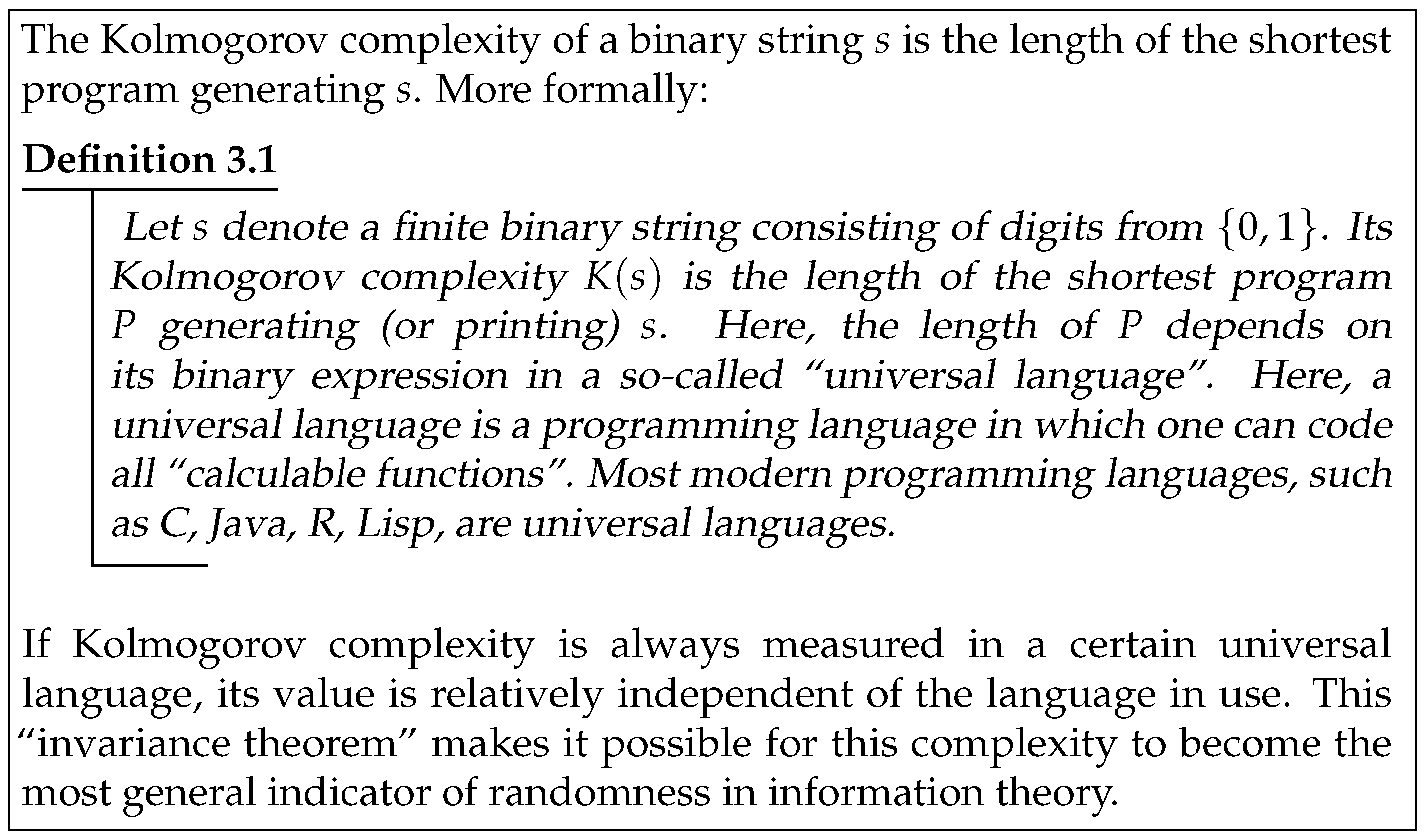
As , s should be attributed to the second case. Remark here that the shorter is a string’s generating rule, the more likely it can be generated by a randomly chosen program.
Thus, to measure the likelihood of generating a binary string
s by pure chance, one needs the length of its describing rule, noted by
m. As
s could be generated by more than one program, we take the shortest one to calculate
m. The length of the shortest program generating
s is defined as the Kolmogorov complexity of
s [
23]. For more details on this concept see
Figure 1.
Reference [
15,
17] make a perfect link between the probability of generating
s by pure chance and its Kolmogorov complexity. If all finite binary strings can be considered as the output of computer programs, the probability to observe
s is given by Equation (
1):
Here,
is the probability to observe
s, and
its Kolmogorov complexity.
is called the semimeasure universal for the class of enumerable semimeasures. Like [
24] we’ll just call it the universal distribution.
The universal distribution proposes the a priori probability of a binary string s, when the sample is generated by randomly picked out programs. This a priori probability should not be attributed to any other theoretical assumption. For financial researchers, it is another “natural” distribution, like the normal or uniform one, that delivers no information on the validity of economic theories.
To make the universal distribution operational, one needs the Kolmogorov complexity of
s. While, despite its general acceptation, Kolmogorov complexity of a finite string cannot be calculated directly (Because of the famous halting problem [
25], for more detail see [
26]). Compression tools can be used to estimate the Kolmogorov complexity of long finite strings. However, as these tools need long data to be efficient, the Kolmogorov complexity of a short string has been difficult to estimate for a long time. Reference [
27] make a progress in this direction. These authors code all existing 5-state programs, and estimate the appearing frequency of each finite string at the output, i.e.,
in Equation (
1). According to
, reference [
27] give a complexity ranking of all binary strings under 7 bits. This ranking is confirmed by 5-state programs in [
20].
Based on this ranking, one can verify the validity of the universal distribution with data from physical world. Reference [
28] made a first application of the universal distribution in Psychology.
To sum up, there are two types of randomness: the normal randomness defined in a mathematical framework and the algorithmic one coming from computer science. Both describe the “natural” state of physical world and neither should be attributed to economic assumptions.
In the next section, we will conduct an empirical study to verify the distribution of financial volatilities. We will show to which degree daily volatilities can be ranked by their complexity. This result explains, at least to some extent, the general presence of VC in financial time series.
4. The Universal Distribution of Stock Volatility
In this section, we use daily returns of common stocks observed from international exchanges to show how well the universal distribution fits volatility data.
Table 1 gives a presentation of our sample. To show the wide presence of the universal distribution, we sampled a price-driven market (NYSE) as well as order-driven ones. Our sample covers more than 20 years of transactions and have been observed from 3 variant continents.
For each exchange, we investigate the components of its market index. The composition of these indexes is fixed on 31 March 2014. All data has been furnished by the commercialized platform IDOS. For each individual stock, daily returns are calculated by the difference of logarithmic Closes, and volatility is the absolute value of successive returns.
Volatilities calculated like this are noted in real numbers. However, the universal distribution is solely relevant to binary strings. To reveal algorithmic structures in financial volatilities, it is necessary to make some data transformation.
In our work, this data transformation is conducted asset by asset. For each individual stock, every trading week is transformed into a 5-bit binary string following 3 steps:
To transform a real number series into a binary one, we take daily volatilities of each stock, and set those above (resp. under) the sample median to be “1” (resp. “0”). Thus, in every binary series, we observe as much “0” (representing small volatilities) as “1” (representing large ones). This property is appreciated in our study since it allows a direct comparison between universal and uniform distributions.
Then, every binary sequence is divided into trading weeks according to civil agenda. When a civil week contains no-trading days, all trading data during this week is deleted from the sample.
The above-described two steps are repeated with each individual stock. The frequency of all possible binary trading weeks is calculated for the 5 exchanges in our sample.
Table 2 exposes the numeric results, and
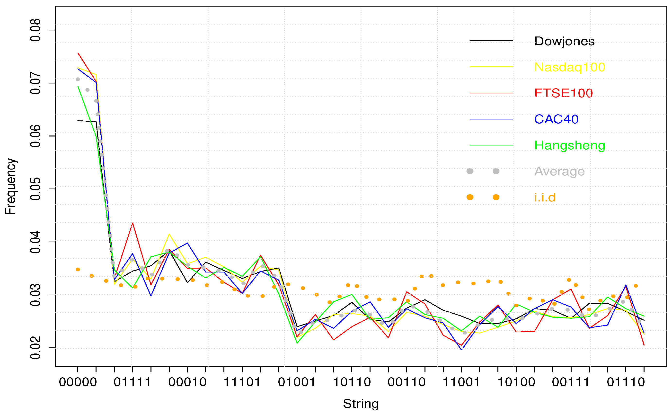
Figure 2 gives an intuitive presentation of them.
Please note that the 32 possible binary trading weeks can be divided into 3 classes, according to their appearing frequency:
“00000” and “11111” are most frequent, since they are the simplest 5-bit strings according to [
27]. Their average frequency is 0.07072 and 0.06692 respectively for the 5 sampled exchanges.
“00001”, “01111”, “10000”, “11110”, “00010”, “01000”, “10111”, “11101”, “00100” and “11011” constitute the second class, with their average frequency ranging from 0.03192 to 0.03890.
The others are even less frequent, with their average frequency varying from 0.02244 to 0.02898, what is interesting to underline here, it that they happen to be the most complex 5-bit strings up to [
27].
Remark that these three classes can be observed from individual exchanges as well as the averaged data. In
Figure 2,
X-axis represents all possible binary weeks ranked by their Kolmogorov complexity. Colorful continual lines give the frequency evolution of individual exchanges. The dotted grey curve describes their average. The dotted orange one is what one should expect from Independent and Identically Distributed random variables.
It is drawn by simulating 100,000 independently and normally distributed successive returns. We note also that binary trading weeks’ frequency diminishes with their Kolmogorov complexity. A significant drop is observed at each class boundary, and binary strings in the same class have similar frequencies. Of course, in the case of , represented by the dotted orange curve, all binary strings have similar appearing frequencies.
Y-axis represents appearing frequencies of binary trading weeks. X-axis reports the complexity rank given by [
27]. We observe here 3 frequency levels: 00000 and 11111 are most frequent as they are the simplest 5-bit binary strings according to their Kolmogorov complexity. The next 10 simplest strings have similar frequencies. And the last 20 strings correspond to the third frequency level.
The over-presence of “00000” and “11111” can be considered as another description of VC than the positive autocorrelation coefficient. Large volatilities are more likely to be followed by large ones, since repetition is simpler than alternation. Even in the second and third classes, more repetitive strings like “00001” or “01111” appear much more frequently than “01101” or “10010”. Hence the principle of the universal distribution: structured strings are more likely to be generated by a random program than complex ones. This result seems indicate that binary trading weeks can be considered, at least partially, as the outputs of randomly chosen programs. This pattern should be attributed to algorithmic randomness not to economic assumptions.
At this step of analysis, it could be interesting to have a discussion on the relationship between the universal distribution and statistical tools. Does algorithmic randomness reveal exactly the same structures as autocorrelation coefficient? In the next section, we will show the complementary role of the universal distribution to econometric models using GARCH simulated data.
5. Algorithmic Randomness and GARCH Simulations
In this section, we study the relationship between algorithmic structure and volatility autocorrelation captured by econometric tools. Firstly, we show that once transformed into binary strings, volatility series simulated from GARCH (1,1) follow a uniform distribution rather than the universal one. Then, we show that the universal distribution of binary trading weeks could lead to autocorrelation of real-number financial volatilities. Thus, the universal distribution could be at the origin of VC, but the volatility autocorrelation cannot result in our reported universal distribution of binary trading weeks.
5.1. The Uniform Distribution of Transformed GARCH Simulated Data
Using “fGARCH” package in “R”, we simulated 100 return series with a GARCH (1,1) model. Although there is a big range of ARCH-type models in the literature, it seems that GARCH (1,1) is not outperformed by more complex models in terms of forecasting power [
29].
Parameters involved in these simulations are
,
. Each simulated series contains 10,000 observations. Once transformed into binary trading weeks, none of the simulated series follows the universal distribution: all binary trading weeks seem to have similar frequencies like what should be observed from an
.
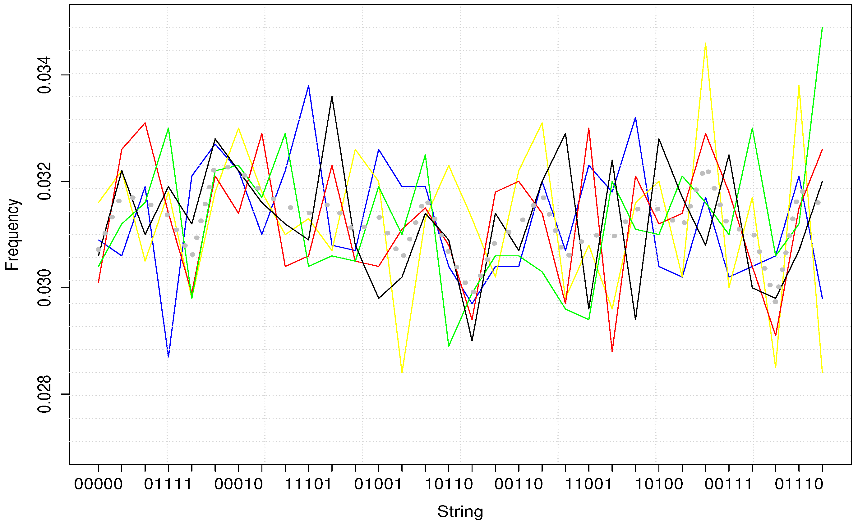
Figure 3 gives an illustration of our result.
In this figure, each colorful line represents one simulated return series. Dotted grey line represents their average. As what we can see from the figure, no frequency difference can be noted from simulated trading weeks.
To some extent, this result should be expected, as econometric models and the universal distribution do not capture the same interaction between successive returns: econometric models estimate the average effect of lagged data on the current one, while the universal distribution focuses on the
structure of historical returns. For example, in econometric models, “0101” and “1010” should not have the same effect on the next volatility. However, according to the universal distribution, these 2 strings have exactly the same structure, so the same impact on the following day. The pattern reported in
Figure 2, cannot be revealed by econometric models but only algorithmic ones.
5.2. The Universal Distribution and Volatility Autocorrelation
If GARCH simulated data cannot be transformed into universally distributed trading weeks, can our reported algorithmic structure result in volatility autocorrelation? A negative answer to this question would indicate a total irrelevance of the universal distribution to VC’s explanation.
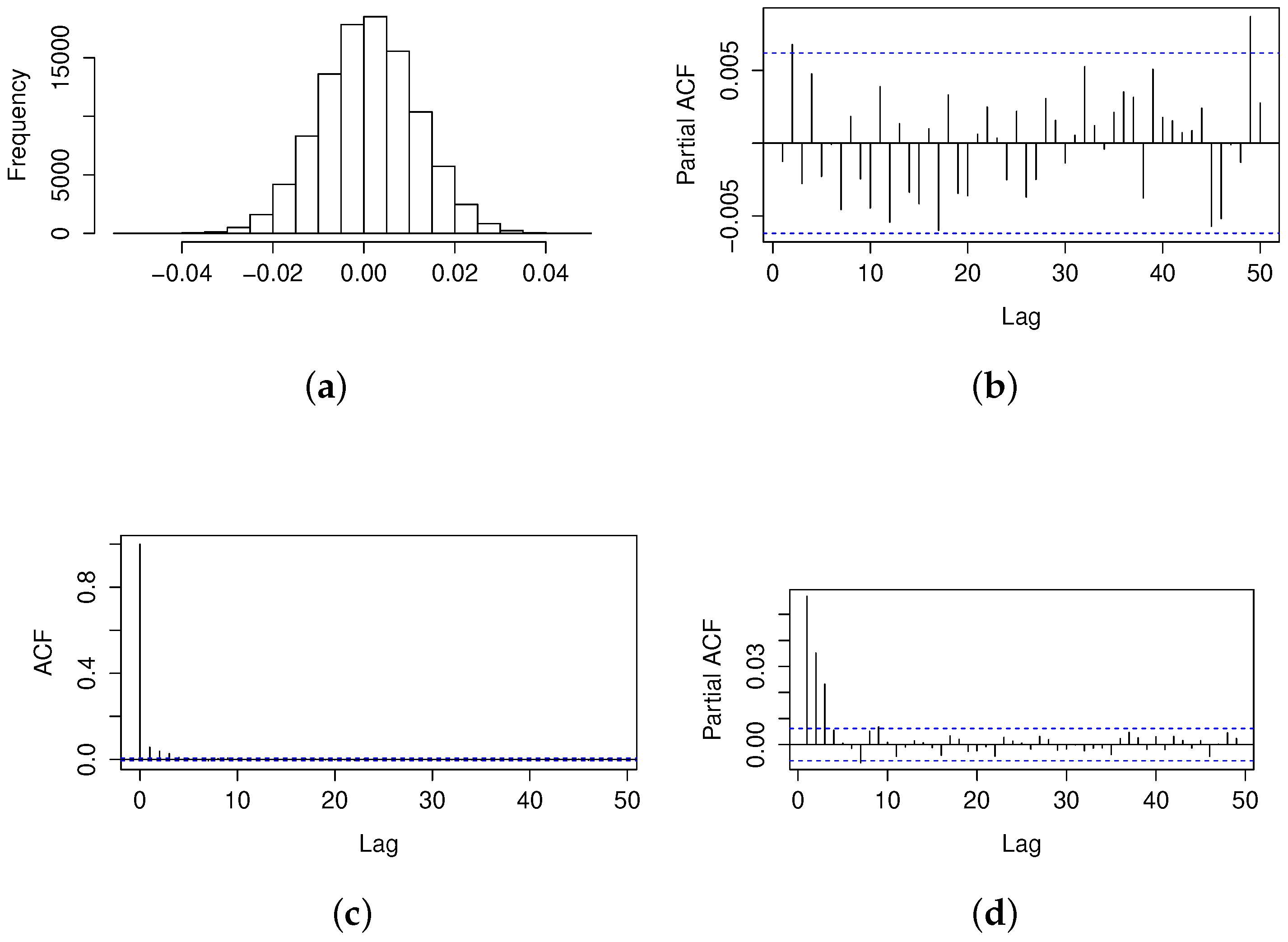
In this section, we show that algorithmic structure reported in our study could be responsible for volatility autocorrelation, and volatility autocorrelation could be solely another way to present the universal distribution of binary weeks.
To do this, we start by simulating 20,000 successive binary weeks. As each week consists of 5 trading days, this will lead to 100,000 daily returns. The binary weeks’ generation depends on the following distribution law:
Like what we exposed in
Table 2, we distinguish three classes of binary weeks: (I) the most frequent class consisting of 2 possible binary strings, (II) the less frequent one consisting of 10 binary weeks, (III) and the least frequent group with the others. The probability associated with each binary week is calculated by taking the average frequency of their corresponding group in
Table 2. For example, we attribute the same probability to“00000” and “11111” that is fixed at
. In the same way, we set the probability of the 10 less frequent strings to be
.
We make 20,000 random draws following the distribution described in
Table 3. The 20,000
100,000 binary trading days obtained like this will be transformed into a volatility series following three steps:
In this section, we attempt to set out the relation between Levin’s universal distribution and the volatility autocorrelation captured by econometric tests. This relation has been investigated in 2 directions: (1) GARCH simulated autocorrelation cannot be the origin of the universal distribution of binary weeks, (2) universal distributed binary weeks do lead to autocorrelations. This result is somewhat expected by the researchers: the universal distribution highlights the origin of VC, while autocorrelation tests is, for us, solely a description of the stylized fact. Algorithmic structure reported in our study gives a more fundamental explanation of VC.
6. Result Discussion
The universal distribution of binary trading weeks have deep significations to financial researchers. Using autocorrelation indicators, [
2,
3] reported VC in financial time series, and since then, the debate on its behavioral or micro-structural origins occupied several decades. Our result indicates another explanation to this widely cited stylized fact: large volatilities are more likely to be followed by large ones, since repetitive binary weeks like “00000” or “11111” are much simpler than alternative ones such as “01011” or “10100”. As simpler strings are more likely to be generated by randomly chosen programs, they should be observed more frequently in the sample. If daily volatilities are not
—thus cannot be attributed to mathematical randomness - their pattern seems to find its origin in algorithmic randomness described by the universal distribution. As algorithmic randomness is another “natural” state of a numeric sample, this result relieves, at least to some extent, VC from economic assumptions.
If the mathematical randomness defined by is a widely accepted notion, the algorithmic one remains rarely mentioned in financial works. Here, it is necessary to make a point on the relation between these 2 types of randomness. After all, what is their conceptional difference, why both should be considered as a “natural” state of empirical data?
As the universal distribution describes binary data, let’s set up this point in a binary framework. According to mathematical randomness, if a binary sample behaves as if someone is tossing a fair coin and recording the output, then, it should be considered as “natural” or “normal”, and has little interest to theoretical researchers. The conceptional origin of this randomness is the coin tossing game.
Meanwhile, the algorithmic randomness described by the universal distribution is another conception: if one gathers all possible computer programs, at each time, he picks out randomly one program to generate a binary trading week, the resulted sample should follow the universal distribution.
To sum up, in a uniform distribution, one picks out randomly one side of a fair coin, while in the universal distribution, one makes the same random choice among all computer programs. Our result indicates that financial volatilities behave as if, at the beginning of each week, someone points at a program randomly, and this program’s output is the binary trading week to follow.
If algorithmic randomness is rarely mentioned in the financial literature, it is not that novel to the physical world. Actually, the world consists of all kinds of interactions: those among molecules, macroscopic objects, biological genes, economic agents, computers, telephones, and so on. These interactions are regulated by different calculating systems (programs) that are working at different levels implicitly or explicitly. If physical objects could be considered as the output of computer programs, it should be “natural” to observe algorithmic “hints” in the physical world (pictures, voice, economic series). This idea defended by [
18,
19,
30] offers a perfect theoretical framework to our study.
Today, financial transactions are primarily arranged by computers. The order executing system and all network infrastructures are organized by computer programs. With the introduction of high frequency trading, even part of the order emitting work is under the responsibility of computer programs. It should not be that surprising to discover some tracks of the universal distribution in transaction records.
With regard to econometric tools, our algorithmic method has several advantages:
Firstly, it qualifies VC as a “natural” state that is to be attributed to algorithmic randomness. However, auto-correlation tests deliver no information on the origin of VC.
Secondly, to characterize VC, econometric models calculate an average impact of lagged observations on the current one. While the universal distribution distinguishes lagged volatilities according their structure. For example, in a GARCH model, “0110” and “1001” cannot have the same impact on the present volatility, while according to the universal distribution, they have exactly the same structure (as “0110” is the inverse of “1001”) and thus the same impact.
Finally, as what we show in the last section, the 3 complexity classes observed from financial volatilities cannot be noted in GARCH simulated returns. However, universally distributed binary weeks do result in volatility autocorrelation.
These tests are conducted to answer an essential question to this paper: Is the universal distribution solely another way to describe volatility autocorrelation or could it be a fundamental explanation of VC?
After all, when we use different tools to capture the same empirical fact, two cases are always possible: (1) each tool takes a different “picture” of the empirical fact, no conversion can be realized between the reported structures. (2) one of the tools reveals the origin of the empirical fact, the pattern detected by this tool is more “fundamental” and will lead to other “pictures”.
As volatility autocorrelation cannot account for the universal distribution of binary weeks, and this algorithmic structure does result in volatility autocorrelation. It should play a more fundamental role in the explanation of VC.
Here, another question one could ask here is that if the universal distribution is a“natural” state of volatilities, why financial returns are not organized in the same? How to distinguish “natural states” described by a uniform distribution from those characterized by the universal one? Let’s begin our analysis with some real-world examples.
It seems that physical objects follow the universal distribution in a general way. In addition, uniform randomness usually occurs under some “heating” conditions.
The same analysis could be brought to financial data. The universal distribution of returns would conduct to excessive profits, permanent arbitrage on returns would push them to a uniform distribution. The permanent arbitrage could be considered as some kind of heating condition. When it comes to volatilities, VC is not directly linked to trading profits, so volatilities will not be “heated” by arbitrages, hence the universal distribution.
Our study answers to a fundamental question in Finance: if no particular micro-structural or rationality assumption is made, and financial returns are randomly delivered by algorithms (not by a fair coin), how do successive returns should be distributed? We argue in the manuscript that the universal distribution seems to be a better answer than the uniform one. Then volatility clusterings become a consequence of the universal distribution of binary trading weeks, totally free of all micro-structural or rationality assumption as it is suggested in the latent literature.
7. Conclusions
In this paper, we attempt to throw some light on the origin of VC on testing the distribution of binary trading weeks. Our investigation begins with the distinction of two types of “natural” states that should be attributed to pure randomness in a binary world: the mathematical one, described by the uniform distribution, and the algorithmic one, characterized by the universal distribution. We argue that if to choose one side of a fair coin is a reasonable conception of randomness, to pick out a computer program could be an as sensible one in a world where calculation regulates most interactions.
With data from five exchanges and covering more than 20 years, we show that, once transformed into binary trading weeks, successive daily volatilities do not follow a uniform distribution but the universal one.
This result indicates that financial volatilities behave as if, at each week, someone picks out a program randomly, and the program’s output is the binary trading week to appear. From a theoretical point of view, our result relieves VC from all micro-structural or behavioral assumptions, in the way that this well referenced stylized fact could be due to the complexity difference between repetitive strings such as “00000” or “11111” and alternative ones such as “01101” or “10010”.
As VC is usually highlighted by autocorrelation functions, we find it necessary to compare the universal distribution to these econometric measures. Empirical tests show that once transformed into binary sets, GARCH-simulated data do not follow the universal distribution, but universally distributed binary weeks do lead to volatility autocorrelation. Thus, volatility dependance cannot be totally captured by GARCH models. The universal distribution reveals some new structure in successive returns that could be at the origin of volatility autocorrelation. This new structure could change the way we conceive financial patterns, and once integrated into a volatility model such as neural systems, it could probably improve the model’s predictive performance.
Despite these new perspectives offered by the algorithmic structure, this study remains a first investigation before more general applications. Although our sample covers 5 exchanges and more than 20 years, it is relatively limited in terms of sample frequency. In a future work, we could study the presence of the universal distribution in intra-day, weekly, or monthly data. These data’s universal distribution could be a further witness of the algorithmic nature of financial volatilities.


