Article

Iterative Identification for Multivariable Systems with Time-Delays Based on Basis Pursuit De-Noising and Auxiliary Model

1
School of Internet of Things Engineering, Jiangnan University, Wuxi 214122, China
2
Key Laboratory of Advanced Process Control for Light Industry (Ministry of Education), Jiangnan University, Wuxi 214122, China
*
Author to whom correspondence should be addressed.
Algorithms 2018, 11(11), 180; https://doi.org/10.3390/a11110180
Submission received: 30 September 2018 / Revised: 27 October 2018 / Accepted: 31 October 2018 / Published: 6 November 2018
(This article belongs to the Special Issue Parameter Estimation Algorithms and Its Applications)

Abstract

:
This paper focuses on the joint estimation of parameters and time-delays of the multiple-input single-output output-error systems. Since the time-delays are unknown, an effective identification model with a high dimensional and sparse parameter vector is established based on overparameterization. Then, the identification problem is converted to a sparse optimization problem. Based on the basis pursuit de-noising criterion and the auxiliary model identification idea, an auxiliary model based basis pursuit de-noising iterative algorithm is presented. The parameters are estimated by solving a quadratic program, and the unavailable terms in the information vector are updated by the auxiliary model outputs iteratively. The time-delays are estimated according to the sparse structure of the parameter vector. The proposed method can obtain effective estimates of the parameters and time-delays from few sampled data. The simulation results illustrate the effectiveness of the proposed algorithm.

1. Introduction

This paper focuses on the identification of the multiple-input single-output output-error systems with unknown time-delays. The investigation is introduced from its background, the formulation of the problem, the literature survey, and the scope and the contributions in this section.

1.1. Background

System identification is a process of developing mathematical models of dynamical systems based on observed data [1]. The dynamical system to be modeled can be a mechanical system, an industrial system or other types of system. Many identification methods have been proposed for the specific systems. For example, some identification techniques for mechanical systems can be found in [2,3,4]. In this paper, we study the identification of multivariable systems because most of the industrial processes can be modeled as multivariable systems.
Multivariable systems are a class of systems which often present significant interactions between the multiple-input and multiple-output channels. A wealth of literature is available on effective identification algorithms for such systems. For example, an expectation-maximization technique was employed for the estimation of the linear time-invariant (LTI) multiple-input multiple-output (MIMO) systems [5]. A matchable-observable linear identification with zero-order oracle filter tuning method was developed for the LTI MIMO systems by comprising the problems of parameter estimation, filter tuning and model structure selection [6]. The methods proposed in [5,6] are applicable for the MIMO systems without time-delays. In many industry processes, time-delays are usually unavoidable. Therefore, it is of great interest to study the identification of multivariable systems with unknown time-delays.
For the estimation of time-delays in multivariable systems, several methods have been proposed. In [7], a parametric model is first estimated by using generalized orthonormal basis filters. Then, the time-delay estimates are generated by analyzing the simulated step response of the resulting model. However, it is required that the model structure is available a priori. To address this problem, a non-parametric method was proposed in [8]. The central idea is to break up a general m × n MIMO system into m n decoupled single-input single-output systems using partial coherence functions, and then to apply the frequency-domain method to estimate the time-delay of each subsystem. Since the time-delay estimation procedure was repeated for m n times, this method requires a large amount of computation and is limited for high order systems. In this paper, we attempt to find a simple and efficient method to address the joint estimation of time-delays and parameters of multivariable systems.

1.2. Formulation of the Problem of Interest for this Investigation

For simplicity, we consider the identification problem of multiple-input single-output output-error (MISO-OE) systems with unknown input time-delays. The main body of the MISO-OE model is the impulse transfer functions between the inputs and output. The identification challenge lies in that the system output is nonlinear in the polynomial parameters.
For the identification of the multivariable systems with time-delays, it is needed to form an appropriate identification model first. Taking into account the unknown time-delays, a high dimensional identification model is formed with a sparse parameter vector, which contains many zeros [9,10]. For the identification of high dimensional models, traditional identification methods, such as the least squares method and the stochastic gradient method, require many observations as well as heavy computational burden. However, there are many situations in reality where only limited observations are available such as setpoint-operated processes, online estimation and linear time-variant system identification [11]. It has proven that traditional identification is unreliable in these cases and the estimates often tend to be biased or have large variances [12]. Therefore, it is necessary to develop new identification methods and reduce the identification cost.
The compressive sensing theory originally arose in the signal processing community, which enables the reconstruction of sparse or compressible signals under the undersampling condition [13]. In view of the sparse characteristic of the identification model, the estimation of the sparse parameter vector can be addressed as a reconstruction problem of the sparse signal.

1.3. Literature Survey

Greedy algorithms and convex optimization approaches are most widely used reconstruction methods. Greedy algorithms are commonly applied for solving minimum l 0 norm problem with advantages of fast speed and easy implement [14]. Convex optimization approaches are a class of global optimization methods, which address minimum l 1 norm problems with high stability and strong applicability [15]. Basis pursuit, basis pursuit de-noising (BPDN) [16], the least absolute shrinkage and selection operator (LASSO) [17], and the least angle regression [18] are typical convex optimization approaches. These approaches can be converted to linear programming or quadratic programming form, and then the optimal solutions can be obtained [19]. Recently, the reconstruction methods have been applied for system identification. For example, the orthogonal matching pursuit algorithm was applied to obtain the joint estimation of parameters and time-delays of the MISO finite impulse response systems and MISO controlled autoregressive systems [20,21]. The compressive sampling matching pursuit algorithm was modified by employing the instrumental variable method to identify a class of closed-loop systems [22]. The LASSO approach is investigated for computing efficient model structure of the overparameterized nonlinear autoregressive, moving average exogenous systems [23]. In this paper, we aim to identify the MISO-OE systems with time-delays based on a convex optimization approach.
Compared with the systems studied in [20,21], the structure of the MISO-OE systems is more general and complex. Considering that the system output is nonlinear in the polynomial parameters, the MISO-OE system model can be transformed into a linear regression form by introducing intermediate variables. However, the intermediate variables are unmeasurable and make the identification difficult. Fortunately, the auxiliary model identification idea can solve this problem by replacing unmeasured variables with outputs of the auxiliary model which is constructed of measurable variables [24]. Combining the auxiliary model idea with conventional methods, many new identification methods have been developed such as the auxiliary model based stochastic gradient algorithm [25], and the auxiliary model based least squares (AM-RLS) algorithm [26]. It is indicated that the AM-RLS algorithm can obtain unbiased and consistent estimation of parameters under a persistent excitation condition. Inspired by the algorithms in [25,26], we attempt to combine the auxiliary model idea with the convex optimization approach to deal with the joint estimation of parameters and time-delays of MISO-OE systems.

1.4. Scope and Contribution of this Study

This investigation deals with the identification of the MISO-OE systems with unknown time-delays based on convex optimization and auxiliary model. The structure of the MISO-OE systems is different from the systems studied in [20,21], which means that different methods need to be applied to form the identification model. In this paper, the auxiliary model technique is employed to address the nonlinearity of parameters, and an effective identification model with a high dimensional and sparse parameter vector is derived due to the unknown time-delays. In addition, a different identification method is applied here. The methods proposed in [20,21] are modifications of a greedy algorithm. In this paper, a convex optimization approach, the BPDN approach, is modified for identification due to its robustness. By converting the BPDN approach to a quadratic programming form, the parameters are calculated from the optimal solutions, and the unmeasurable terms in the information vector are updated iteratively. The unknown time-delays can be read from the estimated parameter vector. The effectiveness of the proposed algorithm is tested by simulation examples.

1.5. Organization of the Paper

The rest of this paper is organized as follows. Section 2 introduces the MISO-OE systems with time-delays and describes the identification problem. Section 3 presents an auxiliary model-basis pursuit de-noising iterative (AM-BPDNI) algorithm. Section 4 provides a simulation example to show the effectiveness of the AM-BPDNI algorithm. Finally, some summaries are given in Section 5.

2. Problem Description

Consider an MISO-OE system
y ( t ) = i = 1 r z d i B i ( z ) A i ( z ) u i ( t ) + v ( t ) ,
where u i ( t ) and d i are the input and time-delay of the ith input channel, y ( t ) is the output, v ( t ) is a white noise vector with zero mean and variance σ 2 , and A i ( z ) and B i ( z ) are the time-invariant polynomials with constant coefficients in the unit backward shift operator z 1 [ i . e . , u ( t ) z 1 = u ( t 1 ) ] ,
A i ( z ) : = 1 + a i 1 z 1 + a i 2 z 2 + + a i n a i z n a i , B i ( z ) : = b i 1 z 1 + b i 2 z 2 + + b i n b i z n b i .
Assume that the orders n a i and n b i are known, y ( t ) = 0 , u i ( t ) = 0 and v ( t ) = 0 for t < 0 .
To form the identification model, an intermediate variable is introduced [24],
x i ( t ) : = z d i B i ( z ) A i ( z ) u i ( t ) = [ 1 A i ( z ) ] x i ( t ) + z d i B i ( z ) u i ( t ) .
Since the time-delay d i of each input channel is unknown, an overparameterization method is applied by setting a maximum input regression length l which satisfies l max ( d i + n b i ) [20]. Then, x i ( t ) can be written in an impact form
x i ( t ) = φ i T ( t ) θ i ,
where
φ i ( t ) : = [ x i ( t 1 ) , x i ( t 2 ) , , x i ( t n a i ) , u i ( t 1 ) , , u i ( t d i ) , u i ( t d i 1 ) , , u i ( t d i n b i ) , , u i ( t l ) ] T R n a i + l ,
θ i : = [ a i 1 , a i 2 , , a i n a i , 0 , , 0 d i , b i 1 , b i 2 , , b i n b i , 0 , , 0 l d i n b i ] T R n a i + l .
The identification model of the system in Equation (1) can be formed as
y ( t ) = i = 1 r x i ( t ) + v ( t ) = φ T ( t ) θ + v ( t ) ,
where
φ ( t ) : = [ φ 1 T ( t ) , φ 2 T ( t ) , , φ r T ( t ) ] T R n ,
θ : = [ θ 1 T , θ 2 T , , θ r T ] T R n ,
n : = i = 1 r ( n a i + l ) .
It can be seen from Equations (3) and (6) that the parameter vector θ contains many zeros, therefore θ is a sparse vector and the system in Equation (4) is a sparse system. The sparsity level can be measured by K : = i = 1 r ( n a i + n b i ) , which denotes the number of non-zero elements in θ . The identification objective is to estimate the unknown parameters a i j , b i j as well as the time-delays d i from observations.

3. Identification Algorithm

If we have m observations from t = 1 to t = m , Equation (4) can be written in a stacked form
Y = Φ θ + V ,
where
Y : = [ y ( 1 ) , y ( 2 ) , , y ( m ) ] T R m ,
Φ : = [ φ ( 1 ) , φ ( 2 ) , , φ ( m ) ] T R m × n , V : = [ v ( 1 ) , v ( 2 ) , , v ( m ) ] T R m .
From Equations (2), (5) and (10), we can see that the information matrix Φ contains many unknown intermediate terms. Therefore, it is difficult to perform the identification directly. According to the auxiliary model identification idea [24,27], the information matrix Φ can be replaced with its estimate
Φ ^ k : = [ φ ^ k ( 1 ) , φ ^ k ( 2 ) , , φ ^ k ( m ) ] T ,
where
φ ^ k ( t ) : = [ φ ^ 1 , k T ( t ) , φ ^ 2 , k T ( t ) , , φ ^ r , k T ( t ) ] T ,
φ ^ i , k ( t ) : = [ x ^ i , k 1 ( t 1 ) , , x ^ i , k 1 ( t n a i ) , u i ( t 1 ) , , u i ( t l ) ] T .
Note that the unmeasurable terms x i ( t j ) are replaced with their auxiliary model output estimates x ^ i ( t j ) . Then, the parameter vector θ can be estimated by the auxiliary model based least squares iterative (AM-LSI) algorithm [28],
θ ^ k = [ Φ ^ k T Φ ^ k ] 1 Φ ^ k T Y , k = 1 , 2 , 3 ,
x ^ 1 , k ( t ) = φ ^ 1 , k T ( t ) θ ^ k ( 1 : n a 1 + l ) ,
x ^ i , k ( t ) = φ ^ i , k T ( t ) θ ^ k 1 + j = 1 i 1 ( n a j + l ) : j = 1 i ( n a j + l ) , i = 2 , 3 , , r ,
where θ ^ k denotes the parameter vector estimate at the kth iteration. According to the least squares (LS) theory, the AM-LSI algorithm is efficient if it is satisfied that m n . However, from Equation (7), we can see that the dimension of the system in Equation (8) is high. Therefore, it would take a lot of time and efforts to obtain enough observations to meet the identification requirement. Moreover, Equation (14) shows that the AM-LSI algorithm requires computing the inverse matrix [ Φ ^ k T Φ ^ k ] 1 at each iteration, which leads to a heavy computational burden. Furthermore, the sparse solution cannot be obtained [23], and the time-delays cannot be effectively estimated. Thus, the AM-LSI algorithm is infeasible for the high dimensional and sparse system identification.
Inspired by the compressive sensing theory, the identification of the sparse system in Equation (8) can be further expressed as an optimization problem
θ ^ = arg min θ 0 , s . t . Y Φ θ 2 2 ε ,
where · 0 represents the l 0 norm, · 2 the l 2 norm, and ε the error tolerance, which is a priori chosen. However, it is a non-convex problem and is difficult to solve in practice. A commonly used alternative is to replace the l 0 norm with a relaxed convex l 1 norm [9],
θ ^ = arg min θ 1 , s . t . Y Φ θ 2 2 ε ,
where · 1 is the l 1 norm. It is proved that the minimization of l 1 norm is equivalent to the minimization of l 0 norm when the Restricted Isometry Property (RIP) is satisfied [13]. Then, the convex optimization problem in Equation (17) is solvable with the BPDN criterion [16]. The BPDN approach can effectively reduce the interference of noise and has good robustness. Inspired by the auxiliary model and the iterative identification idea in the AM-LSI algorithm, we apply the BPDN criterion to modify the AM-LSI algorithm by replacing the LS step with the BPDN criterion. The parameters are estimated by the BPDN criterion and the unmeasurable terms are replaced by the outputs of the auxiliary model in each iteration.
Let k = 1 , 2 , be the iterative number. To get accurate reconstruction from Equation (17), the information matrix should satisfy some conditions, such as the RIP [29] or the exact recovery condition (ERC) [9]. The ERC guarantee and the consistency properties for the identification of the controlled autoregressive models have been investigated in [12]. To meet the ERC, we normalize the information matrix Φ ^ k defined in Equations (11)–(13) by dividing the elements in each column by the l 2 norm of that column [30,31]. Denote the element of the ith row and jth column in Φ ^ k by Φ ^ k , i j , and the normalized information matrix Φ ^ k , n is constructed by
Φ ^ k : = Φ ^ k , n Φ ^ l 2 , Φ ^ l 2 : = Φ ^ k ( 1 ) 0 0 0 Φ ^ k ( 2 ) 0 0 0 Φ ^ k ( n ) R n × n ,
where Φ ^ k ( j ) : = i = 1 m ( Φ ^ k , i j ) 2 . Similarly, the normalized parameter vector θ k , n can be defined as
θ n : = Φ ^ l 2 θ .
Note that the location of non-zeros in θ n is identical to that in θ . Accordingly, the constrained optimization problem in Equation (17) equals
θ ^ n = arg min θ n 1 , s . t . Y Φ ^ k , n θ n 2 2 ε .
The problem in Equation (20) is closely related to the following unconstrained convex optimization problem
θ ^ n = min θ n 1 2 Y Φ ^ k , n θ n 2 2 + λ θ n 1 ,
where λ is a nonnegative parameter. Since the information matrix Φ ^ k is normalized, we can set λ to the value λ = σ 2 log ( n ) [16].
The key step of the BPDN approach is to express Equation (21) as a quadratic program (QP) problem [32]. To begin with, two nonnegative vectors u n and v n are introduced to express θ n . Let θ n j , u n j and v n j be the jth element of the vectors θ n , u n and v n , respectively, where u n j 0 and v n j 0 for all j = 1 , 2 , , n . Define
u n j : = ( θ n j ) + , v n j : = ( θ n j ) + , ( ) + : = max { 0 , } .
Then, θ n can be rewritten as
θ n = u n v n .
Accordingly, the l 1 regularization term θ n 1 can be expressed as
θ n 1 = 1 n T u n + 1 n T v n = 1 2 n T z n ,
where 1 n T : = [ 1 , , 1 ] R n , 1 2 n T : = [ 1 , , 1 ] R 2 n , and
z n : = [ u n T , v n T ] T R 2 n .
Note that all elements in z n are nonnegative. Similarly, the quadratic error term can be written as
Y Φ ^ k , n θ n 2 2 = Y [ Φ ^ k , n , Φ ^ k , n ] z n 2 2 = Y T Y Y T [ Φ ^ k , n , Φ ^ k , n ] z n z n T [ Φ ^ k , n , Φ ^ k , n ] T Y + z n T [ Φ ^ k , n , Φ ^ k , n ] T [ Φ ^ k , n , Φ ^ k , n ] z n .
Since Y T [ Φ ^ k , n , Φ ^ k , n ] z n is a scalar, it follows that
Y T [ Φ ^ k , n , Φ ^ k , n ] z n = ( Y T [ Φ ^ k , n , Φ ^ k , n ] z n ) T = z n T [ Φ ^ k , n , Φ ^ k , n ] T Y = [ Y T Φ ^ k , n , Y T Φ ^ k , n ] z n .
Let
b : = Φ ^ k , n T Y R n .
Equation (24) can be further written as
Y Φ ^ k , n θ n 2 2 = Y T Y 2 [ b T , b T ] z n + z n T [ Φ ^ k , n , Φ ^ k , n ] T [ Φ ^ k , n , Φ ^ k , n ] z n = Y T Y 2 [ b T , b T ] z n + z n T Φ ^ k , n T Φ ^ k , n Φ ^ k , n T Φ ^ k , n Φ ^ k , n T Φ ^ k , n Φ ^ k , n T Φ ^ k , n z n = Y T Y 2 [ b T , b T ] z n + z n T b z n ,
where
b : = Φ ^ k , n T Φ ^ k , n Φ ^ k , n T Φ ^ k , n Φ ^ k , n T Φ ^ k , n Φ ^ k , n T Φ ^ k , n R 2 n × 2 n .
From Equations (22) and (26), we have
min θ n 1 2 Y Φ ^ k , n θ n 2 2 + λ θ n 1 = min z n 1 2 Y T Y [ b T , b T ] z n + 1 2 z n T b z n + λ 1 2 n T z n = min z n 1 2 Y T Y + C T z n + 1 2 z n T b z n ,
where
C : = λ 1 2 n + [ b T , b T ] T = σ 2 log ( n ) 1 2 n + [ b T , b T ] T R 2 n .
Since 1 2 Y T Y is a constant, Equation (28) can be constructed in a standard QP framework,
min z n C T z n + 1 2 z n T b z n , s . t . z n j 0 , j = 1 , 2 , , n .
For the inequality constrained QP problem in Equation (30), the common solution is the active set method [33]. While for the sake of simplicity, the QP problem can be directly solved by calling the relevant function from the standard scientific software toolbox. For example, the MATLAB toolbox provides a function “quadprog”. Then, the parameter vector θ ^ n can be obtained from the optimum solution z ^ n ,
θ ^ n = z ^ n ( 1 : n ) z ^ n ( n + 1 : 2 n ) ,
where z ^ n ( 1 : n ) represents a vector formed by the first n elements of z ^ n , and z ^ n ( n + 1 : 2 n ) a vector formed by the last n elements of z ^ n . Considering that the system in Equation (8) is contaminated with noise, the parameter estimation error can be large. To further reduce the estimation error, a small threshold TH = ϵ can be set to filter the elements close to zero in θ ^ n . Let θ ^ n j = 0 if θ ^ n j < ϵ and denote the filtered parameter vector as θ ^ n , ϵ . Then, the parameter vector estimate θ ^ k can be recovered according to Equation (19),
θ ^ k = Φ ^ l 2 1 θ ^ n , ϵ .
The estimates of the intermediate variables x i , k ( t ) can be refreshed by θ ^ k as shown in Equations (15) and (16).
Equations (9), (11)–(13), (15), (16), (18), (23), (25), (27), and (29)–(32) form the auxiliary model-basis pursuit de-noising iterative (AM-BPDNI) algorithm for the MISO-OE system. The implementation procedures are listed as follows:
  • Collect the input–output data { u i ( t ) , y ( t ) : i = 1 , 2 , , r ; t = 1 , 2 , , m } and set the parameter estimation accuracy ε 0 .
  • Construct the stacked output vector Y by Equation (9).
  • Initialize the iteration: let k = 1 and x ^ i , 0 ( t ) be random sequences.
  • Construct the information matrix Φ ^ k by Equations (11)–(13) and normalize Φ ^ k by (18).
  • Form the vectors and matrix z n , b, b and C by Equations (23), (25), (27), and (29) and formulate the QP by Equation (30).
  • Call the function to obtain the optimum solution z ^ n and compute θ ^ n by Equation (31).
  • Set a threshold to obtain θ ^ n , ϵ and recover the parameter vector estimate θ ^ k by (32).
  • Compare θ ^ k with θ ^ k 1 : if θ ^ k θ ^ k 1 > ε 0 , update the auxiliary model outputs x i , k ( t ) by Equations (15) and (16) and go to Step 4. Otherwise, stop the iteration and obtain the parameter vector estimate θ ^ .
The unknown time-delay of each input channel can be estimated according to the location of zero-blocks and the number of zeros in θ ^ . It can be seen from Equations (3) and (6) that there are 2 r zero-blocks in θ ^ . Denote the number of zeros in each zero-block by z i ( i = 1 , 2 , , 2 r ) . Then, time-delays can be estimated by
d ^ i = z 2 i 1 , i = 1 , 2 , , 2 r .

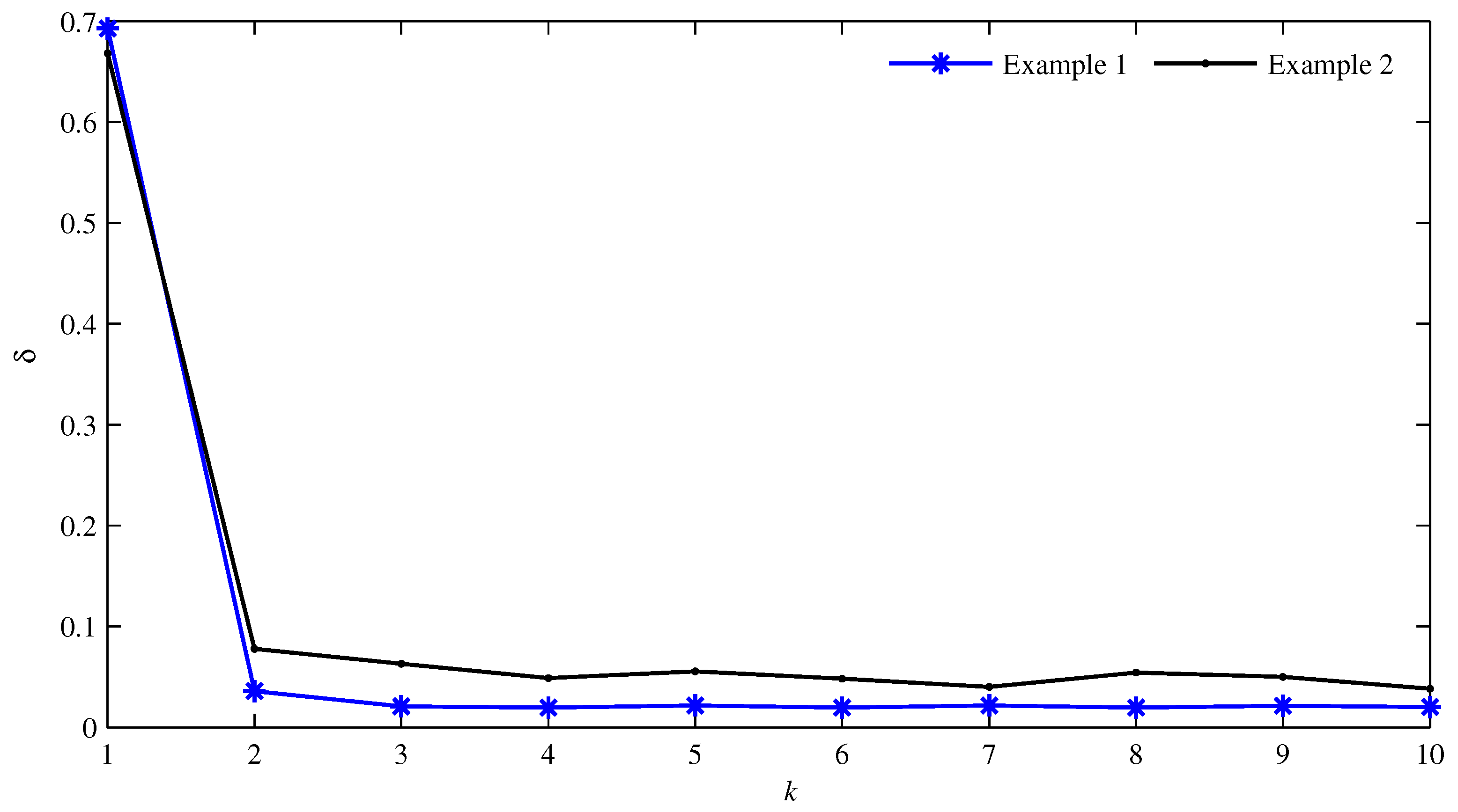
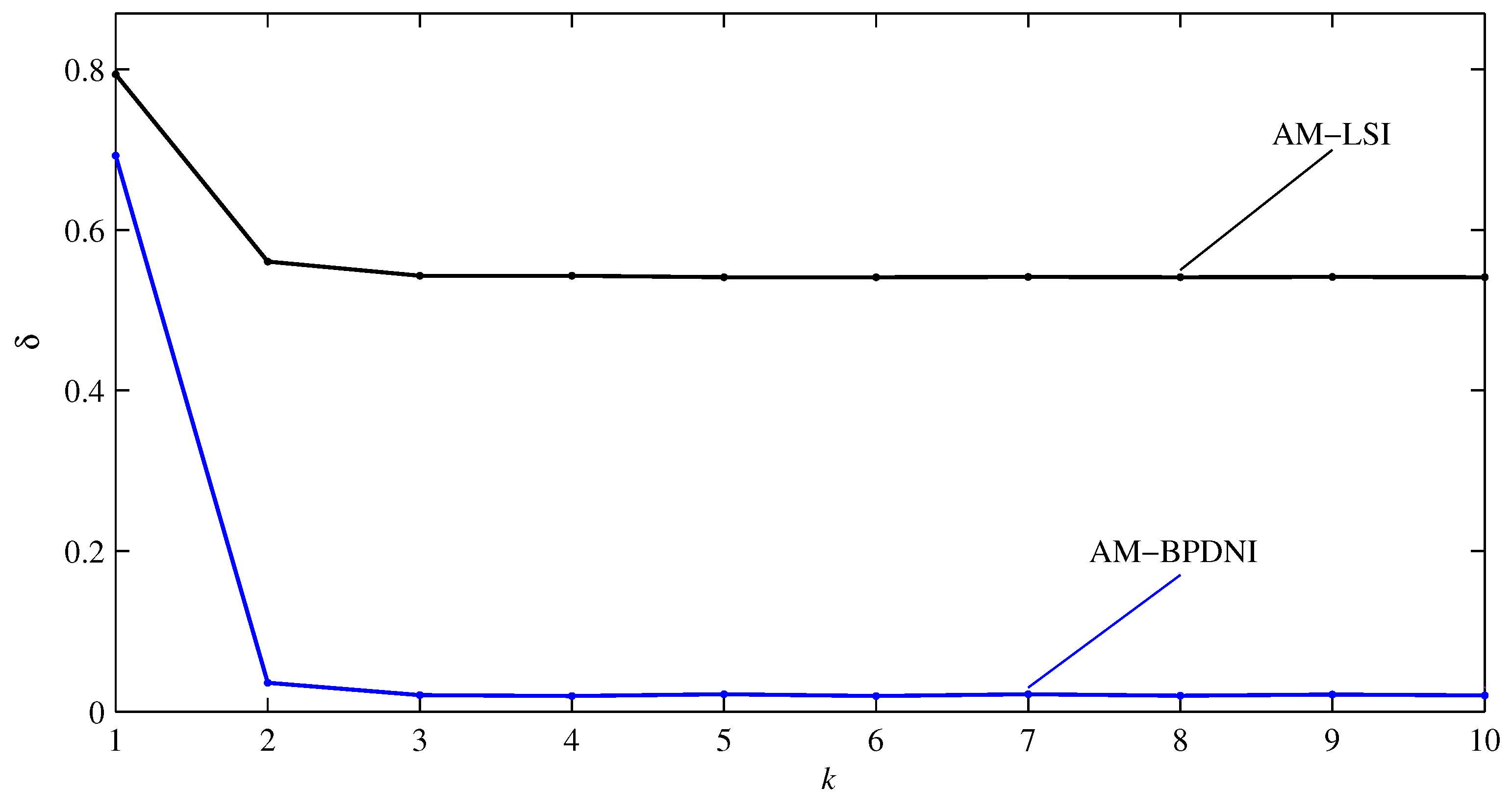
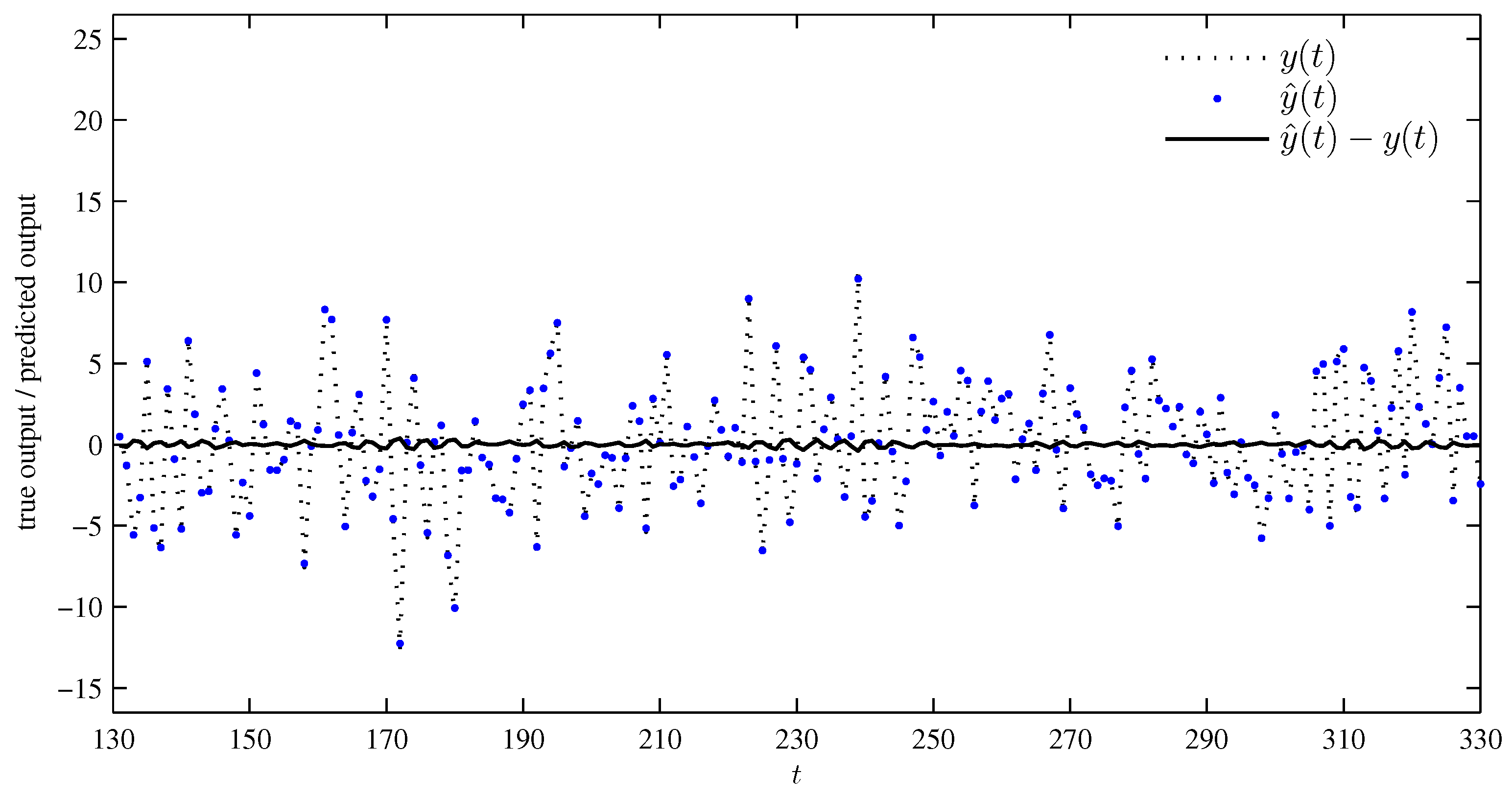
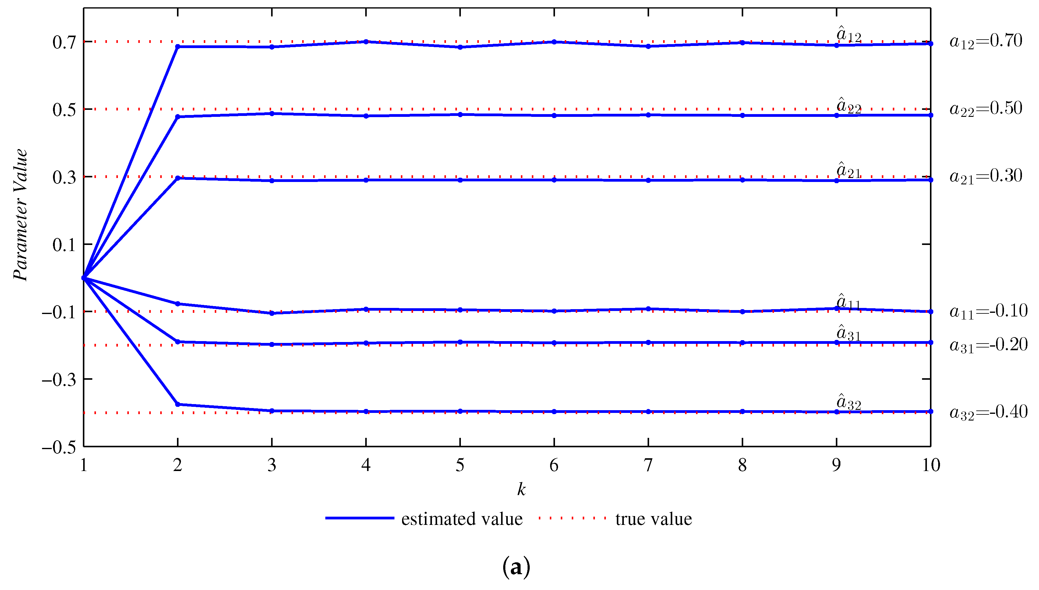
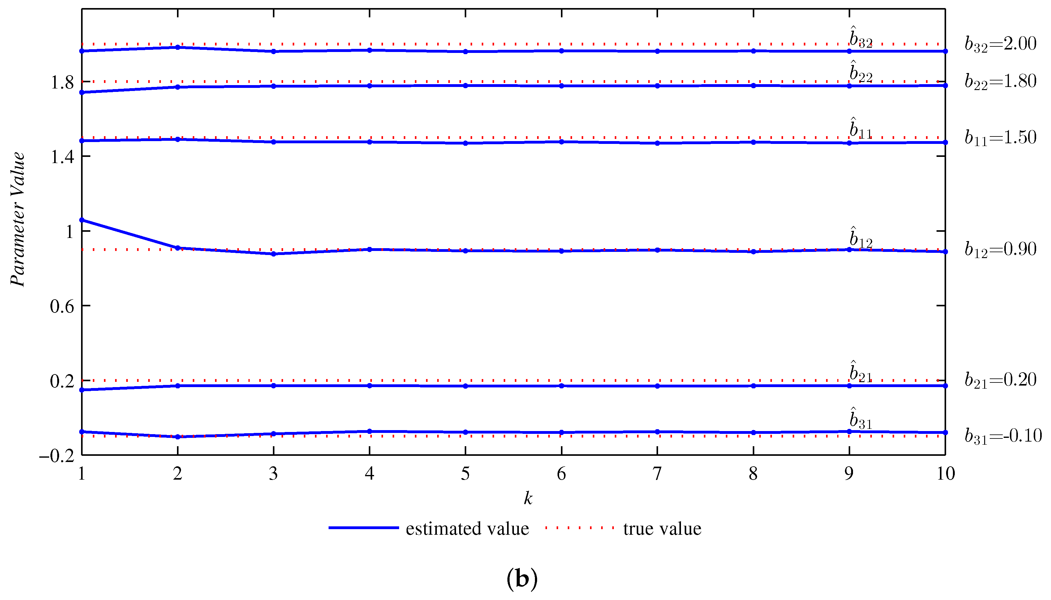
4. Simulation Example

Example 1.
Consider the following MISO-OE system with time-delays,
y ( t ) = i = 1 3 z d i B i ( z ) A i ( z ) u i ( t ) + v ( t ) , A 1 ( z ) = 1 0.1 z 1 + 0.7 z 2 , B 1 ( z ) = 1.5 z 1 + 0.9 z 2 , A 2 ( z ) = 1 + 0.3 z 1 + 0.5 z 2 , B 2 ( z ) = 0.2 z 1 + 1.8 z 2 , A 3 ( z ) = 1 0.2 z 1 0.4 z 2 , B 3 ( z ) = 0.1 z 1 + 2 z 2 , d 1 = 20 , d 2 = 10 , d 3 = 30 .
The system in Equation (34) is a second order system with three inputs and one output. The inputs { u i ( t ) } , i = 1 , 2 , 3 are taken as random uncorrelated signal sequences with zero mean and unit variances, and { v ( t ) } as a white noise sequence with zero mean and variances σ 2 . Let the maximum input regression length be l = 50 . Then, the parameter vector to be identified is
θ 1 = [ 0.1 , 0.7 , 0 20 , 1.5 , 0.9 , 0 28 , 0.3 , 0.5 , 0 10 , 0.2 , 1.8 , 0 38 , 0.2 , 0.4 , 0 30 , 0.1 , 2 , 0 18 ] T R 156 ,
where 0 i denotes the zero-block with i zeros. Note that the number of non-zero elements is K = θ 0 = i = 1 3 ( n a i + n b i ) = 12 .
Taking m = 130 and TH = 0.001 , apply the AM-LSI algorithm and the AM-BPDNI algorithm to perform the identification, respectively. The parameter estimation errors δ : = θ θ ^ / θ versus different noise levels are shown in Table 1. When σ 2 = 0.10 2 , the estimation errors δ versus the iterative number k are shown in Figure 1. It can be seen that the AM-BPDNI algorithm performs better than the AM-LSI algorithm and is insensitive to noise.
Let the variance of { v ( t ) } be σ 2 = 0.10 2 . Apply the AM-BPDNI algorithm to obtain the estimated model of the system in Equation (34) with the first m = 130 data. Then, validate the estimated model by using m e = 200 samples from t = 131 to 330. The predicted output of the estimated model, the true output of the system and their errors are plotted in Figure 2. It is shown that the predicted outputs y ^ ( t ) are close to the true outputs y ( t ) . Moreover, the average predicted output error
δ v : = 1 m e t = 131 330 [ y ^ ( t ) y ( t ) ] 2 = 0.1422
is small and close to the standard deviation of the noise σ = 0.10 . It follows that the estimated model can well capture the system dynamics.
Let m = 130 and σ 2 = 0.10 2 . Using the AM-BPDNI algorithm to estimate the sparse parameter vector θ , the non-zero parameter estimates versus k are shown in Table 2 and Figure 3.
With 10 iterations, the estimated parameter vector is
θ ^ 1 = [ 0.1001 , 0.6938 , 0 20 , 1.4737 , 0.8882 , 0 28 , 0.2902 , 0.4818 , 0 10 , 0.1699 , 1.7783 , 0 38 , 0.1917 , 0.3961 , 0 30 , 0.08002 , 1.9628 , 0 18 ] T .
It can be seen from Equation (35) that there are six zero-blocks in θ ^ and the number of zeros in each zero-block are z 1 = 20 , z 2 = 28 , z 3 = 10 , z 4 = 38 , z 5 = 30 and z 6 = 18 . Then, the time-delay of each input channel can be estimated according to Equation (33),
d ^ 1 = z 1 = 20 , d ^ 2 = z 3 = 10 , d ^ 3 = z 5 = 30 .
Obviously, the time-delay estimates are agreement with the true time-delays.
Example 2.
Consider the following MISO-OE system with time-delays,
y ( t ) = i = 1 4 z d i B i ( z ) A i ( z ) u i ( t ) + v ( t ) , A 1 ( z ) = 1 0.1 z 1 + 0.7 z 2 , B 1 ( z ) = 1.5 z 1 + 0.9 z 2 , A 2 ( z ) = 1 + 0.3 z 1 + 0.5 z 2 , B 2 ( z ) = 0.2 z 1 + 1.8 z 2 , A 3 ( z ) = 1 0.2 z 1 0.4 z 2 , B 3 ( z ) = 0.1 z 1 + 2 z 2 , A 4 ( z ) = 1 0.4 z 1 0.1 z 2 , B 4 ( z ) = 1.1 z 1 + 0.8 z 2 , d 1 = 20 , d 2 = 10 , d 3 = 30 , d 4 = 40 .
Compared with the system in Equation (34), the system in Equation (36) has one more input. Thus, the number of parameters is increased. Let l = 50 and the true parameter vector is
θ 2 = [ 0.1 , 0.7 , 0 20 , 1.5 , 0.9 , 0 28 , 0.3 , 0.5 , 0 10 , 0.2 , 1.8 , 0 38 , 0.2 , 0.4 , 0 30 , 0.1 , 2 , 0 18 , 0.4 , 0.1 , 0 40 , 1.1 , 0.8 , 0 8 ] T R 208 .
Taking m = 130 , σ 2 = 0 . 10 2 , and TH = 0.001 , employ the AM-BPDNI algorithm to identify the system in Equation (36). The estimated parameter vector is
θ ^ 2 = [ 0.0874 , 0.6849 , 0 20 , 1.4682 , 0.9218 , 0 28 , 0.2880 , 0.4711 , 0 10 , 0.1658 , 1.7708 , 0 38 , 0.1842 , 0.3968 , 0 30 , 0.0759 , 1.9503 , 0 18 , 0.4563 , 0.0556 , 0 40 , 1.0429 , 0.7457 , 0 8 ] T .
The time-delay estimates are
d ^ 1 = z 1 = 20 , d ^ 2 = z 3 = 10 , d ^ 3 = z 5 = 30 , d ^ 4 = z 7 = 40 ,
which are identical to the true time-delays.
The parameter estimation errors of the systems in Equations (34) and (36) versus k are shown in Figure 4.
The running time of the proposed method for the systems is t 1 = 1.374637 s and t 2 = 2.398602 s. It can be concluded that the computational burden increases as the dimension of the parameter vector increases.
The simulation results show that for the MISO-OE model, the proposed AM-BPDNI algorithm can obtain efficient estimation of parameters from few observations ( m < n ) with good robustness. Moreover, the AM-BPDNI algorithm can effectively estimate the time-delays according to the sparse characteristic of the estimated parameter vector. However, as the number of the input channels increases, the computational burden of the proposed algorithm increases.

5. Conclusions

This paper proposes an AM-BPDNI algorithm for the identification of MISO-OE systems with unknown time-delays. Based on the BPDN criterion and the auxiliary model identification idea, the sparse parameters and multiple-input time-delays can be effectively and simultaneously estimated. The proposed algorithm requires few sampled data and is robust to noise.

Author Contributions

J.Y. wrote the manuscript. Y.L. revised the manuscript.

Funding

This research was funded by the National Natural Science Foundation of China (Nos. 61304138 and 61473136) and the Jiangsu Province Industry University Prospective Joint Research Project (BY2015019-29).

Conflicts of Interest

The authors declare no conflict of interest.

References

  1. Prochazka, A.; Kingsbury, N.; Payner, P.J.W.; Uhlir, J. Signal Analysis and Prediction; Birkhäuser Basel: Boston, MA, USA, 1998. [Google Scholar]
  2. Pappalardo, C.M.; Guida, D. System identification algorithm for computing the modal parameters of linear mechanical systems. Machines 2018, 6, 12. [Google Scholar]
  3. Pappalardo, C.M.; Guida, D. System identification and experimental modal analysis of a frame structure. Eng. Lett. 2018, 2018 26, 56–68. [Google Scholar]
  4. Pappalardo, C.M.; Guida, D. A time-domain system identification numerical procedure for obtaining linear dynamical models of multibody mechanical systems. Arch. Appl. Mech. 2018, 88, 1325–1347. [Google Scholar] [CrossRef]
  5. Gibson, S.; Ninness, B. Robust maximum-likelihood estimation of multivariable dynamic systems. Automatica 2005, 41, 1667–1682. [Google Scholar] [CrossRef] [Green Version]
  6. Romano, R.A.; Pait, F. Matchable-observable linear models and direct filter tuning: an approach to multivariable identification. IEEE Trans. Autom. Control 2017, 62, 2180–2193. [Google Scholar] [CrossRef]
  7. Patwardhan, S.C.; Shah, S.L. From data to diagnosis and control using generalized orthonormal basis filters. Part I: Development of state observers. J. Process Control 2005, 15, 819–835. [Google Scholar] [CrossRef]
  8. Selvanathan, S.; Tangirala, A.K. Time-delay estimation in multivariate systems using Hilbert transform relation and partial coherence functions. Chem. Eng. Sci. 2010, 65, 660–674. [Google Scholar] [CrossRef]
  9. Tropp, J.A. Just relax: Convex programming methods for identifying sparse signals in noise. IEEE Trans. Inf. Theory 2006, 52, 1030–1051. [Google Scholar] [CrossRef]
  10. Elad, M. Sparse and Redundant Representations: From Theory to Applications in Signal and Image Processing; Springer: New York, NY, USA, 2010. [Google Scholar]
  11. Sanandaji, B.M.; Vincent, T.L.; Wakin, M.B.; Tóth, R.; Poolla, K. Compressive system identification of LTI and LTV ARX models. In Proceedings of the 50th IEEE Conference on Decision and Control and European Control Conference, Orlando, FL, USA, 12–15 December 2011; pp. 791–798. [Google Scholar]
  12. Tóth, R.; Sanandaji, B.M.; Poolla, K.; Vincent, T.L. Compressive system identification in the Linear Time-Invariant framework. In Proceedings of the 50th IEEE Conference on Decision and Control and European Control Conference, Orlando, FL, USA, 12–15 December 2011; pp. 783–790. [Google Scholar]
  13. Donoho, D.L. Compressed Sensing. IEEE Trans. Inf. Theory 2006, 52, 1289–1306. [Google Scholar] [CrossRef]
  14. Tropp, J.A.; Gilbert, A.C.; Strauss, M.J. Algorithms for simultaneous sparse approximation. Part I: Greedy pursuit. Signal Process. 2006, 86, 572–588. [Google Scholar] [CrossRef]
  15. Tropp, J.A. Algorithms for simultaneous sparse approximation. Part II: Convex relaxation. Signal Process. 2006, 86, 589–602. [Google Scholar] [CrossRef] [Green Version]
  16. Chen, S.S.; Donoho, D.L.; Saunders, M.A. Atomic decomposition by basis pursuit. SIAM Rev. 2001, 43, 129–159. [Google Scholar] [CrossRef]
  17. Tibshirani, R. Regression shrinkage and selection via the lasso. J. R. Statist. Soc. Ser. B (Methodological) 1996, 58, 267–288. [Google Scholar]
  18. Efron, B.; Hastie, T.; Johnstone, I.; Tibshirani, R. Least angel regression. Ann. Statist. 2004, 32, 407–451. [Google Scholar]
  19. Boyd, S.; Vandenberghe, L. Convex Optimization; Cambridge University Press: New York, NY, USA, 2004. [Google Scholar]
  20. Liu, Y.J.; Tao, T.Y. A CS recovery algorithm for model and time delay identification of MISO-FIR systems. Algorithms 2015, 8, 743–753. [Google Scholar] [CrossRef]
  21. Liu, Y.J.; Tao, T.Y.; Ding, F. Parameter and time-delay identification for MISO systems based on orthogonal matching pursuit algorithm. Control Decis. 2015, 30, 2103–2107. [Google Scholar]
  22. Liu, Y.J.; H, X.; Ding, F. An instrumental variable based compressed sampling matching pursuit method for closed-loop identification. Control Decis. 2017, 32, 1837–1843. [Google Scholar]
  23. Sánchez-Peña, R.S.; Casín, J.Q.; Cayuela, V.P. Identification and Control: The Gap Between Theory and Practice; Springer: London, UK, 2007. [Google Scholar]
  24. Ding, F.; Chen, T. Combined parameter and output estimation of dual-rate systems using an auxiliary model. Automatica 2004, 40, 1739–1748. [Google Scholar] [CrossRef]
  25. Liu, Q.Y.; Ding, F. The data filtering based generalized stochastic gradient parameter estimation algorithms for multivariate output-error autoregressive systems using the auxiliary model. Multidimens. Syst. Signal Process. 2018, 29, 1781–1800. [Google Scholar] [CrossRef]
  26. Wang, Y.J.; Ding, F. Novel data filtering based parameter identification for multiple-input multiple-output systems using the auxiliary model. Automatica 2016, 71, 308–313. [Google Scholar] [CrossRef]
  27. Wang, Y.J.; Ding, F. The filtering based iterative identification for multivariable systems. IET Control Theory Appl. 2016, 10, 894–902. [Google Scholar] [CrossRef]
  28. Ma, J.X.; Ding, F.; Yang, E.F. Data filtering-based least squares iterative algorithm for Hammerstein nonlinear systems by using the model decomposition. Nonlinear Dyn. 2016, 83, 1895–1908. [Google Scholar] [CrossRef] [Green Version]
  29. Cand‘es, E.J.; Romberg, J.; Tao, T. Robust uncertainty principles: exact signal reconstruction from highly incomplete frequency information. IEEE Trans. Inf. Theory 2006, 52, 489–509. [Google Scholar] [CrossRef] [Green Version]
  30. Wang, W.X.; Yang, R.; Lai, Y.C.; Kovanis, V.; Grebogi, C. Predicting catastrophes in nonlinear dynamical systems by cmpressive sensing. Phys. Rev. Lett. 2011, 106, 154101. [Google Scholar] [CrossRef] [PubMed]
  31. Naik, M.; Cochran, D. Nonlinear system identification using compressed sensing. In Proceedings of the 2012 Conference Record of the Forty Sixth Asilomar Conference on Signals, Systems and Computers, Pacific Grove, CA, USA, 4–7 November 2012; pp. 426–430. [Google Scholar]
  32. Figueiredo, M.A.T.; Nowak, R.D.; Wright, S.J. Gradient projection for sparse reconstruction: Application to compressed sensing and other inverse problems. IEEE J. Sel. Top. Signal Process. 2007, 1, 586–597. [Google Scholar] [CrossRef]
  33. Nocedal, J.; Wright, S.J. Numerical Optimization, 2nd ed.; Springer: New York, NY, USA, 2006. [Google Scholar]
Figure 1. The parameter estimation error δ versus k ( m = 130 , σ 2 = 0.10 2 ).
Algorithms 11 00180 g001
Figure 2. Predicted output y ^ ( t ) , true output y ( t ) and errors (from t =131 to 330).
Algorithms 11 00180 g002
Figure 3. (a) The parameter estimates a ^ ij versus k. (b) The parameter estimates b ^ ij versus k. The non-zero parameter estimates versus k with m = 130, σ 2 = 0.102.
Algorithms 11 00180 g003aAlgorithms 11 00180 g003b
Figure 4. The parameter estimation errors δ of different systems versus k.
Algorithms 11 00180 g004
Table 1. The parameter estimation errors δ (%) versus the noise variances σ 2 ( m = 130 ).
σ 0.100.150.200.250.300.40
AM-LSI53.428453.717554.275355.333755.843557.2966
AM-BPDNI1.99742.98254.79858.66658.95129.8808
Table 2. The non-zero parameter estimates and estimation error δ versus k ( m = 130 , σ 2 = 0.10 2 ).
k a 11 a 12 b 11 b 12 a 21 a 22 b 21 b 22 a 31 a 32 b 31 b 32 δ (%)
10.0000.0001.4831.0580.0000.0000.1481.7420.0000.000–0.0761.96369.2788
2–0.0770.6851.4910.9080.2960.4770.1701.771–0.190–0.375–0.1041.9833.5707
5–0.0950.6841.4700.8930.2890.4840.1681.778–0.190–0.396–0.0781.9602.1595
10–0.1000.6941.4740.8880.2900.4820.1701.778–0.192–0.396–0.0801.9631.9974
True value–0.1000.7001.5000.9000.3000.5000.2001.800–0.200–0.400–0.1002.000

