A Machine Learning View on Momentum and Reversal Trading

Abstract

Momentum and reversal effects are important phenomena in stock markets. In academia, relevant studies have been conducted for years. Researchers have attempted to analyze these phenomena using statistical methods and to give some plausible explanations. However, those explanations are sometimes unconvincing. Furthermore, it is very difficult to transfer the findings of these studies to real-world investment trading strategies due to the lack of predictive ability. This paper represents the first attempt to adopt machine learning techniques for investigating the momentum and reversal effects occurring in any stock market. In the study, various machine learning techniques, including the Decision Tree (DT), Support Vector Machine (SVM), Multilayer Perceptron Neural Network (MLP), and Long Short-Term Memory Neural Network (LSTM) were explored and compared carefully. Several models built on these machine learning approaches were used to predict the momentum or reversal effect on the stock market of mainland China, thus allowing investors to build corresponding trading strategies. The experimental results demonstrated that these machine learning approaches, especially the SVM, are beneficial for capturing the relevant momentum and reversal effects, and possibly building profitable trading strategies. Moreover, we propose the corresponding trading strategies in terms of market states to acquire the best investment returns.

1. Introduction

Momentum and reversal effects are common and interesting phenomena in stock markets. The momentum effect means that the stocks that have performed well, i.e., given higher returns, in the past (winners) will probably continue to outperform those that have performed poorly in the past (losers) in the future. On the contrary, the reversal effect represents that the past losers may convert to the winners in the future.

The reversal effect was first observed by [1], in which it was found that buying losers and selling winners might acquire superior returns on the US stock market, because the US market easily overreacts to some events, which results in abnormal price movements. The momentum effect, which claims that buying winners and selling losers at the same time could earn significant positive returns over holding periods of 3–12 months on the US stock market, was discovered by [2].

Up until recently, many relevant studies have been conducted. In addition to the US market, researchers stated that stock markets in different regions have varying degrees of momentum and/or reversal effect(s). For example, Reference [3] observed the momentum effect in the Latin American emerging markets. Reference [4] found evidence of a substantial momentum effect in the China Shanghai stock market over the period from 1995 to 2005. Reference [5] proposed a contrarian portfolio strategy that could obtain profits on the Malaysian stock market based on the short-term reversal effect. Reference [6] pointed out short-term reversal and mid-term momentum effects in weekly stock returns in the European markets. Reference [7] presented profitable arbitrage strategies built on the short-term reversal effect on the Hong Kong stock market.

On top of these observations, various studies [8,9,10,11,12] have been trying to explain the mechanisms behind the effects. For instance, Reference [8] showed that the momentum effect may be correlated to the past trading volume. Reference [9] concluded that the fundamental finance factors have important links with the reversal effect for stocks traded on the Australian Stock Exchange. Reference [5] argued that the market state has a strong relationship with the momentum effect on the Indian equity market. In addition, some researchers have sought to explain the phenomena via behavioral finance models, such as [11,12].

The existence of momentum and reversal effects have challenged the Efficient Markets Hypothesis (EMH). In other words, investors may take the extra yield if they can predict which effect may happen in the next market period. Unfortunately, the concluded results of most of the existing studies are highly dependent on human experience and settings, e.g., within specific market observation and holding periods. Their findings tend to be unrepeatable in other periods. As a result, the effects they observed indeed existed in the past may disappear in the future. Similarly, the summarized factors that explain the effects are not very robust. These links may not be persistent when applied to other market periods. Thus, it is difficult to transfer these research outputs to real-world investment trading.

Nowadays, machine learning, as one of the most important approaches in artificial intelligence, is a very hot research topic in academia as well as in industry. Many pieces of evidence report that machine learning has been applied widely to diverse domains [13,14]. Machine learning is capable of automatically recognizing potentially useful patterns in financial data [15].

The purpose of this paper is to propose the use of machine learning approaches instead of the traditional statistical methods (e.g., the Causality Test and Hypothesis Test) that have been used in previous studies to investigate the momentum and reversal effects on the stock market. To the best of our knowledge, little research has applied machine learning to this problem. In this research, we regard the problem as a supervised machine learning task. This paper presents several models built on various popular machine learning approaches, including the Decision Tree (DT), Support Vector Machine (SVM), Multilayer Perceptron Neural Network (MLP), and Long Short-Term Memory Neural Network (LSTM), to learn historical data and to predict the effects in the next period. Among the various machine learning approaches, the DT learning methods are designated to the construction of decision trees to transform observations of each example/item to draw conclusions about the targeted value of the relevant example/item. It is one of the most widely used predictive modeling approaches for data mining, machine learning, and statistics. Besides, the SVM are supervised learning models that are used in machine learning with associated algorithms to perform critical analyses on the underlying data for classification or regression tests. The conventional SVM approach has been extensively applied in many real-life applications including financial forecasting, image or voice recognition [16,17], etc. Furthermore, the MLP and LSTM are neural network models that are mostly used for time series prediction in numerous real-world applications, while the convolutional neural network (CNN) approach is most commonly used to analyze the complex relationships between pixels for image or video processing. Essentially, CNN uses a variation of the MLP to carry out minimal preprocessing for the input image or video files. Recently, other research studies have tried to adapt the CNN models for financial forecasting. On top of this, Reference [18] proposed an improved bacterial chemotaxis optimization (IBCO) technique for integration into the back propagation neural network to develop a more efficient forecasting model for stock prediction. Obviously, a diverse range of trading strategies involving different machine learning approaches can be developed and thoroughly evaluated. However, due to the limited resources and time at hand, we specifically consider several basic and commonly used models of the DT, SVM, MLP, and LSTM approaches for our preliminary investigation in this manuscript. In addition, it is worth noting that the testing data sets employed in this research study include the China Securities Index 300 (CSI 300) as a capitalization-weighted stock market index to reflect the overall performance of China’s top 300 and most liquid A-share stocks traded on the Shanghai and Shenzhen stock exchanges. The CSI 300 was carefully chosen as China is one of the fast-growing stock markets with great volatility in the past.

In this paper, Section 2 presents the definition of the problem and proposed methods. Section 3 describes the experiment in detail. All the collected experimental results are thoroughly considered and discussed in Section 4 and Section 5. Finally, the concluding remarks are given in Section 6.

2. Materials and Methods

2.1. Problem Description

Momentum and reversal effects can be studied via observation and holding periods. According to customary notations in previous studies, the observation period is defined as J, while the holding period is defined as K. They can be in hours, days, or months. Obviously, different observation and/or holding periods will hugely impact the results. For some pairs of periods, the result might show effects. However, the previously observed patterns might disappear in other periods. Thus, the selection of J and K is very important.

In this paper, J and K were 5, 10, …20 days, i.e., $J,K\in \left[5,10,15,20\right]$.

$$O{R}_i^T={{\displaystyle \prod }}_{t=T+1}^{T+J}\left(r_i^t+1\right)-1$$

(1)

$$H{R}_i^T={{\displaystyle \prod }}_{t=T+J+1}^{T+J+K}\left(r_i^t+1\right)-1$$

(2)

In (1) and (2), $O{R}_i^T$ is the total return of the ith stock in the observation period (J), while $H{R}_i^T$ is the total return of the ith stock over the holding period (K). $r_i^t$ is the daily return of the ith stock on the ith transaction day. $T$ represents the starting day of the observation period.

Stocks in a pre-defined asset pool may be ordered by their returns in the observation period. The top $N$ candidates with the highest returns are regarded as winners, whilst the top $N$ with the lowest returns are marked as losers. As for momentum trading, the winners in the observation period (J) will be selected to build a portfolio, and then hold them until the end of the holding period (K). On the contrary, the losers will be selected to build a portfolio for the reversal trading.

$$R_O^T=\frac{{{\displaystyle \sum }}_{i=1}^{N}O{R}_i^T}{N}=\frac{{{\displaystyle \sum }}_{i=1}^N\left({{\displaystyle \prod }}_{t=T+1}^{T+J}\left(r_i^t+1\right)-1\right)}{N}$$

(3)

$$R_H^T=\frac{{{\displaystyle \sum }}_{i=1}^{N}H{R}_i^T}{N}=\frac{{{\displaystyle \sum }}_{i=1}^N\left({{\displaystyle \prod }}_{t=T+J+1}^{T+J+K}\left(r_i^t+1\right)-1\right)}{N}$$

(4)

Thus, we may calculate the average returns of the portfolio (winners or losers) in J and K, respectively, according to (3) and (4), i.e., $R_O^T$ and $R_H^T$.

In this research, we built prediction models using four proposed machine learning techniques to predict the effect (momentum, reversal, or no effect) that may happen in the next holding period. After that, corresponding strategies were generated based on these predicted signals.

2.2. Decision Tree

DT is a very famous supervised learning technique. It uses a tree-like graph or model to make decisions. Given training data, DT is able to learn decision rules inferred from the data features during the training process.

DT is simple to understand and to interpret. The generated rules can be visualized easily. In addition, DT is very fast, and there is little data preparation for DT.

DT has been widely applied to operations research to help make decisions. In this research, DT was used as one of the machine learning techniques to identify the momentum and reversal effects. As a result, DT can help to make financial decisions, i.e., betting on a momentum or reversal effect. The C4.5 algorithm, an extension of ID3, was adopted in this research. Compared with ID3, the C4.5 algorithm can handle both continuous and discrete data features.

2.3. Support Vector Machine

SVM, one of powerful machine learning algorithms, has achieved success in various domains, such as [15,19,20,21].

The principle of SVM is to minizine the structural risk. SVM is very applicable to classification problems. As described in [22], the mechanism of SVM for classification as follows:

$$\max {{\displaystyle \sum }}_{i=1}^n{\alpha }_i-\frac{1}{2}{{\displaystyle \sum }}_{i=1}^n{{\displaystyle \sum }}_{j=1}^n{\alpha }_i{\alpha }_j{y}_i{y}_{j}k\left(x_i,x_j\right)$$

$$s.t. 0\le {\alpha }_i\le C, i\in \left[1,2,\dots ,n\right]$$

$${{\displaystyle \sum }}_{i=1}^n{\alpha }_i{y}_i=0.$$

(5)

In (5), $k\left(x_i,x_j\right)$ is the kernel function, while $C$ is the penalty factor.

$$f\left(x\right)=sgn\left({{\displaystyle \sum }}_{i=1}^n{a}_i^{*}{y}_{i}k(x_i,x\right)+{\beta }^{*}),$$

(6)

$$k\left(x_i,x\right)=\exp (-\gamma |{|x-x_i|}^2).$$

(7)

SVM can overcome overfitting problems [23]. Essentially, SVM uses the kernel function to project the inputs into high-dimensional feature spaces so that SVM can efficiently solve non-linear classification problems, as shown in (6). In this research, we selected the radial basis function (RBF) as the kernel function, as described in (7).

In addition, there are variants of the SVM approach being applied to a diverse range of application domains. Examples include the fuzzy SVM (FSVM) [24,25,26] and the twin SVM (TWSVM) [27,28]. As numerous industrial applications may contain fuzzy or noisy data, the FSVM tackles the relevant fuzzy information of the underlying applications. In [25], a novel approach combining the wavelet contour analysis for backbone detection, wavelet packet entropy, and FSVM for spine classification was successfully applied and carefully studied. Moreover, another novel advanced fuzzy SVM (NA-FSVM) method was proposed and used to predict the trends of stock prices. On the other hand, the TWSVM approach intrinsically determines two nonparallel hyperplanes such that each hyperplane is closest to one of the two classes yet as far as possible from another class. Essentially, the TWSVM targets two smaller sized quadratic programming problems (QPPs) whereas the conventional SVM targets one larger QPP. Thus, the TWSVM generally works faster than the conventional SVM approach.

2.4. Multilayer Perceptron Neural Network

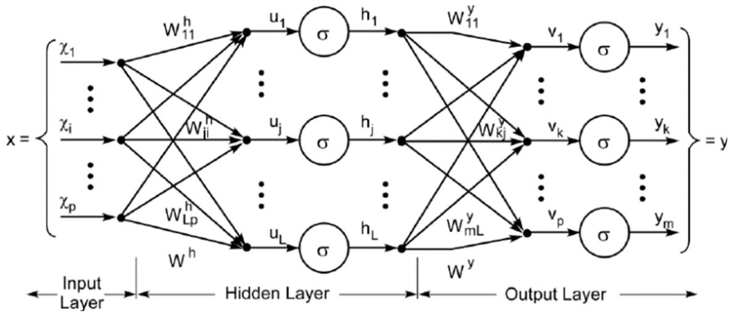
MLP is one of the Deep Artificial Neural Networks (DNNs). MLP has more than one perception. It is composed of an input layer, an arbitrary number of hidden layers, and an output layer, as shown in Figure 1. The input layer receives the signal, while the output layer makes a prediction about the input. The hidden layers provide the computational functions of the MLP.

MLP has been widely applied to supervised learning problems. The model is trained to learn the correlations between inputs and outputs. The model adjusts the parameters, weights, and bases from time to time to minimize errors in the training process.

Designing a good network topology for the studied problem is a tough task. The numbers of layers and neurons on each layer and the selection of activation functions all affect the performance of the model. In practice, we have to try various topologies to acquire a good one. Figure 2 presents the proposed topology after tuning in, for which we tried a few combinations (i.e., the network topologies, the number of layers and neurons, and the activation and loss functions) and picked a good one for this problem. Our MLP model is composed of five layers, i.e., an input layer, an output layer, and three hidden dense layers.

2.5. Long Short-Term Memory Neural Network

LSTM is a powerful architecture of the Recurrent Neural Network (RNN). Compared with the traditional RNN, LSTM overcomes the issue of gradient vanishing. On hidden layers, there are no connections between the neurons, but LSTM introduces memory cells to retain long-term and short-term memory. As price changes may affect price changes in the future, no matter whether they have occurred recently or a long time ago, LSTM is expected to be a suitable algorithm for financial prediction.

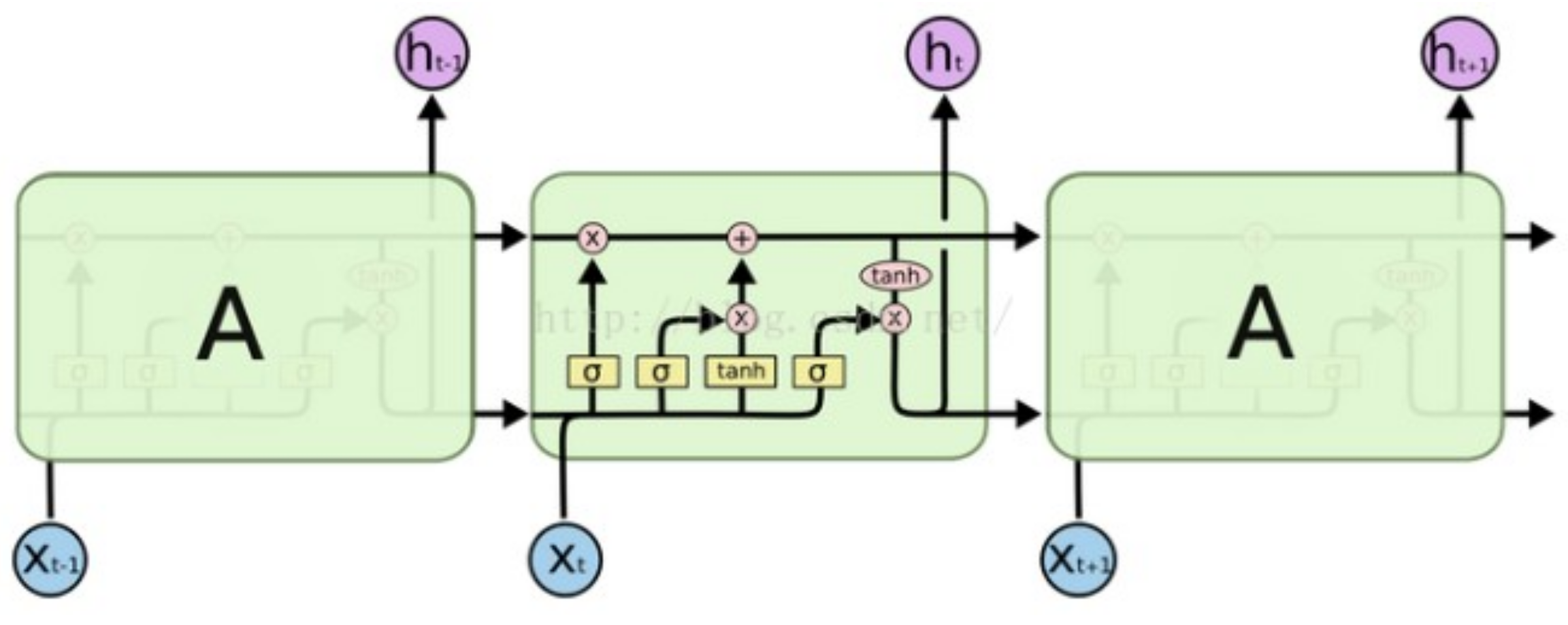
There are three gates in LSTM, input, output, and forget gates, as shown in Figure 3. The function of the forget gate is to forget some memory depending on the current input $x_t$, the last state $c_{t-1},$ and the last output $h_{t-1}$. The role of the input gate is to decide which values can enter the current state $c_t$ up to $x_t$, $c_{t-1}$, and $h_{t-1}$ [22].

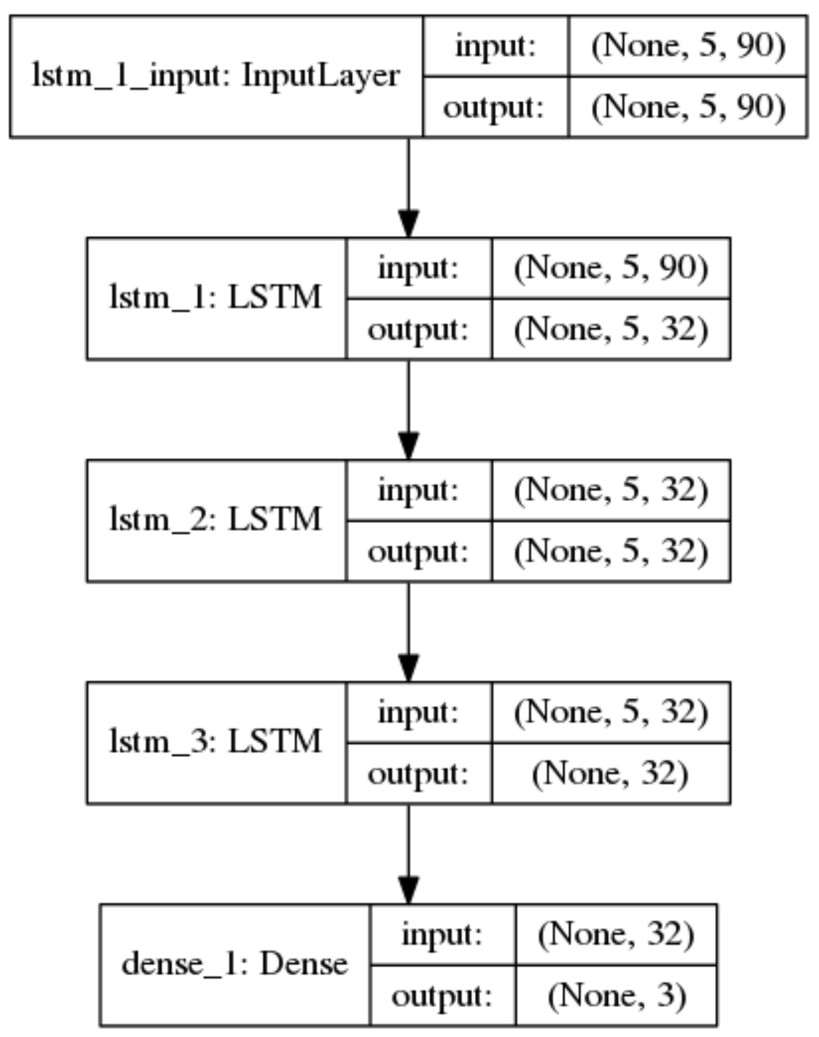
Similar to the ceaseless tuning conducted for the MLP model, our proposed LSTM model is composed of one single input layer, followed by three LSTM layers and a dense output layer. Figure 4 illustrates the proposed topology of our LSTM model. The first layer is the input layer with the input shape (5, 90), i.e., the lookback step is set to 5 after tuning. The second layer is an LSTM layer with the Relu activation function. The following third and fourth layers are LSTM layers with the Sigmoid activation functions. The number of neurons in the hidden LSTM layers is 32. The final layer is a dense layer that is used to output the classification result using the Softmax function.

3. Experiment Setup

3.1. Data Preparation

In this research, we investigated the CSI 300 constituents, which are 300 selected stocks listed on China Shanghai and Shenzhen Stock Exchanges. The CSI 300 constituents comprise the important CSI 300 index. Since the CSI 300 constituents include major value and growth stocks, the study is very significant and meaningful to real-world investment.

All data was acquired from SINA Finance via the opensource tool Tushare [31]. In addition, data cleaning was conducted carefully to remove missing and exotic values.

In order to examine the performance by the models at different market states (i.e., bullish, bearish, and fluctuating markets), the selected ranges of training and testing data covered at least one complete market cycle, respectively, as listed in

Table 1. Ranges of the training and testing data.

Training Data	Testing Data
2007-01-04 to 2011-12-31	2012-01-06 to 2016-02-05

.

3.2. Feature Extraction

Features play an important role in almost all machine learning problems. We extracted a total of 90 input features in this research, as listed in

Table 2. Feature extraction.

Feature Sets
amplitude	market_cap	mom_ps	rev_amplitude	rev_roc
amplitude_std	market_cap_std	mom_ps_std	rev_amplitude_std	rev_roc_std
cci	mom_amplitude	mom_roc	rev_cir_cap	rev_turnover
change	mom_amplitude_std	mom_roc_std	rev_cir_cap_std	rev_turnover_std
cir_cap	mom_cir_cap	mom_turnover	rev_current_rtn	rev_yield_dispersion
cir_cap_std	mom_cir_cap_std	mom_turnover_std	rev_current_rtn_std	rev_yield_dispersion_std
close	mom_current_rtn	mom_yield_dispersion	rev_lb	roc
current_rtn	mom_current_rtn_std	mom_yield_dispersion_std	rev_lb_std	roc_std
current_rtn_std	mom_lb	obv	rev_market_cap	rsi
ema	mom_lb_std	open	rev_market_cap_std	sar
high	mom_market_cap	pb	rev_pb	sma
hurst	mom_market_cap_std	pb_std	rev_pb_std	turnover
kdj_slow_d	mom_pb	pcf	rev_pcf	turnover_std
kdj_slow_k	mom_pb_std	pcf_std	rev_pcf_std	vol_change
lb	mom_pcf	pe	rev_pe	volume
lb_std	mom_pcf_std	pe_std	rev_pe_std	willr
low	mom_pe	ps	rev_ps	yield_dispersion
macd	mom_pe_std	ps_std	rev_ps_std	yield_dispersion_std

. The features included market quotes (e.g., prices (open, high, low, close), volume, turnover, etc.), calculated technical indicators (e.g., the Exponential Moving Average (EMA), the Relative Strength Index (RSI), the Rate-of-Change (ROC), the Moving Average Convergence/Divergence (MACD), etc. In addition, the financial and business states of the listed companies are important factors that react to market prices. Thus, the input features also included some fundamental indicators, such as Market Capitalization (Market Cap), the Price-Earnings Ratio (PE), the Price-to-Book Ratio (PB), the Price-To-Sales Ratio (PS), the Price Cash Flow Ratio (PCF), etc.

In addition to the CSI 300 index, we put the past winners and losers into the momentum (MOM) and reversal (REV) groups, respectively. Then, the above indicators together with some mathematical statistics, such as the mean and standard deviation values, were calculated to generate corresponding features.

3.3. Trading Decisions Process

The momentum and reversal effects might occur over any market duration. However, the difficulty is that these effects do not often occur alternately because the market has neither a momentum effect nor a reversal effect for some periods of time.

Thus, the predicted target by the machine learning models is the prediction of what happens in the next defined market period: momentum effect, reversal effect or no effect. After that, the corresponding trading strategies are picked to build the investment positions: buying winners for the predicted momentum effect, buying losers for the predicted reversal effect or just an empty position for no effect.

Given the training data, the models learned the patterns from history. The prediction process was conducted for the testing data.

3.4. Backtesting

In the experiment, we examined different observation and holding periods to investigate the momentum and reversal effects.

At first, prediction models were built based on the above-proposed machine learning approaches. Then, we conducted backtestings by different models for the testing data. We tried different combinations of observation and holding periods for each model. Finally, the paper trading returns, as indicated in (8), and the Sharpe ratios, as shown in (9), were calculated and compared carefully.

$$R_p= \frac{P_t}{P_0}-1,$$

(8)

$$SR=\frac{{{\displaystyle \sum }}_{i=1}^n\left(R_H^i\right)/n-R_f/365}{\sqrt{\frac{1}{n-1}{{\displaystyle \sum }}_{i=1}^n{\left(R_H^i-\overline{R}\right)}^2}}$$

(9)

where $p_0$. is the intial Net Asset Value (NAV) of the portfolio, whose value was set to 1.0 at the beginning of time, while $p_t$ is the NAV at the end of time $t$. $R_H^i$ is the daily return on the ith day, while $R_f$ is the risk-free rate.

Since transaction costs are very important factors that may affect the investing return dramatically in real-world trading, we had to take into account these costs in the backtesting for the better market trading simulation. The transaction costs and risk-free rate are listed in

Table 3. Transaction costs and risk-free rate.

Brokerage Commission	Tax	Risk-Free Rate
0.03% of the transaction per trade	0.1% of the transaction when selling stocks	3.00%

.

4. Results

4.1. Performance of the Buy-and-Hold Strategy

In financial investment, the related market index is normally a benchmark to measure the performance of proposed trading strategies. As our studied objects were CSI 300 constitutes, the CSI 300 index was our benchmark.

We built a buy-and-hold strategy that bought and held the CSI 300 index at the beginning of the backtest until the end of the backtesting. The return and Sharpe ratio of the buy-and-hold strategy were 30.27% and 0.37, respectively, as listed in

Table 4. Performance of the buy-and-hold strategy.

Buy-and-Hold Strategy Return	Buy-and-Hold Strategy Sharpe Ratio
30.27%	0.37

.

4.2. Performance of the Momentum and Reversal Trading Strategies

Two standalone trading strategies, the momentum strategy and the reversal strategy, were backtested as well. The momentum strategy suggests always buying the winners observed in the past period (J) and holding them until the end of future period (K). The reversal strategy is the opposite to the momentum strategy.

Finally, the paper trade returns and Sharpe ratios were calculated and are listed in

Table 5. Performance of the momentum and reversal trading strategies.

J	K	Momentum Strategy Return	Momentum Strategy Sharpe Ratio	Reversal Strategy Return	Reversal Strategy Sharpe Ratio
5	5	−2.89%	0.12	75.21%	0.62
	10	0.22%	0.16	21.09%	0.31
	15	−16.00%	0.00	124.32%	0.85
	20	86.15%	0.68	60.81%	0.56
10	5	−28.93%	−0.12	38.00%	0.42
	10	13.25%	0.26	12.78%	0.24
	15	1.26%	0.16	109.25%	0.79
	20	107.73%	0.76	36.83%	0.42
15	5	−8.25%	0.10	34.50%	0.40
	10	49.16%	0.49	16.86%	0.28
	15	−1.48%	0.14	63.16%	0.57
	20	116.55%	0.79	75.22%	0.64
20	5	−33.78%	−0.15	−0.87%	0.14
	10	18.96%	0.30	10.20%	0.23
	15	−28.35%	−0.12	88.61%	0.70
	20	74.01%	0.62	65.24%	0.58

.

4.3. Performance of the Decision Tree Model

Table 6. Performance of the Decision Tree (DT) model.

J	K	DT Model Return	DT Model Sharpe Ratio
5	5	22.62%	0.32
	10	9.42%	0.18
	15	42.93%	0.49
	20	47.92%	0.50
10	5	−9.00%	0.05
	10	68.40%	0.64
	15	24.47%	0.32
	20	52.81%	0.60
15	5	175.90%	1.52
	10	207.17%	1.34
	15	50.59%	0.60
	20	100.33%	0.92
20	5	13.65%	0.21
	10	36.24%	0.41
	15	27.14%	0.35
	20	21.07%	0.29

shows the backtesting performance of the DT model. With the help of this machine learning model, the momentum, reversal or empty strategy was selected in advance in accordance with the description in Section 3.3. Similarly, different combinations of J and K were investigated as well.

4.4. Performance of the SVM Model

Table 7. Performance of the Support Vector Machine (SVM) model.

J	K	SVM Model Return	SVM Model Sharpe Ratio
5	5	67.38%	0.62
	10	60.15%	0.62
	15	15.00%	0.22
	20	128.55%	1.12
10	5	96.70%	0.90
	10	58.06%	0.60
	15	0.74%	0.00
	20	60.29%	0.66
15	5	89.33%	0.90
	10	239.43%	1.68
	15	5.40%	0.09
	20	179.36%	1.39
20	5	42.44%	0.52
	10	120.19%	1.06
	15	−37.43%	−0.60
	20	114.08%	1.00

lists the backtesting results of the SVM model where the model achieved the best performance with a return of 239.43% and a Sharpe ratio of 1.68 when J was 15 and K was 10.

4.5. Performance of the MLP Model

Table 8. Performance of the Multilayer Perceptron Neural Network (MLP) model.

J	K	MLP Model Return	MLP Model Sharpe Ratio
5	5	23.75%	0.32
	10	47.53%	0.49
	15	49.57%	0.51
	20	74.50%	0.71
10	5	139.37%	0.97
	10	56.23%	0.57
	15	28.62%	0.36
	20	34.17%	0.40
15	5	105.95%	0.92
	10	215.26%	1.41
	15	−24.52%	−0.22
	20	70.21%	0.69
20	5	33.01%	0.39
	10	70.40%	0.66
	15	29.60%	0.36
	20	29.26%	0.36

lists the backtesting results of the MLP model where the model achieved the best performance with a return of 215.26% and a Sharpe ratio of 1.41 when J was 15 and K was 10.

4.6. Performance of the LSTM Model

Table 9. Performance of the LSTM model.

J	K	LSTM Model Return	LSTM Model Sharpe Ratio
5	5	10.75%	0.21
	10	129.96%	1.06
	15	−20.85%	−0.19
	20	201.30%	1.25
10	5	−17.63%	−0.14
	10	51.07%	0.54
	15	2.30%	0.10
	20	92.83%	0.74
15	5	−4.23%	0.03
	10	106.98%	0.98
	15	112.93%	0.85
	20	42.05%	0.53
20	5	12.46%	0.24
	10	8.16%	0.19
	15	−32.40%	−0.31
	20	38.60%	0.43

lists the backtesting results of the LSTM model where the model achieved the best performance with a return of 201.30% and a Sharpe ratio of 1.25 when J was 5 and K was 20.

4.7. Comparison of the Net Asset Values of the Portfolios

In order to investigate the dynamic performance during the whole backtesting duration, we plotted the NAV curves of the portfolios suggested by the best strategies.

Figure 5, Figure 6, Figure 7 and Figure 8 present the NAV curves generated by the best strategies in the DT, SVM, MLP, and LSTM models. In each figure, the NAV curves of the best standalone momentum and reversal strategies are compared with that of the machine learning model.

In addition to the NAV curve of the buy-and-hold strategy, Figure 9 puts all curves together so that we can make comparisons across the best strategies produced by the machine learning models and standalone momentum and reversal trading.

5. Discussion

5.1. Examination of Momentum and Reversal Effects

From Table 5, we can see that the results differed from each other in terms of different combinations of J and K. For the momentum strategy, the pair of (J = 15, K = 20) achieved the best performance with a return of 116.55% and a Sharpe ratio of 0.79, whilst the pair of (J = 5, K = 15) achieved a return of 124.32% and a Sharpe ratio of 0.85 for the reversal trading. These strategies bet the benchmark strategy, i.e., the buy-and-hold strategy that had a return of 30.27% and a Sharpe ratio of 0.37.

However, the returns and Sharpe ratios for some periods were even worse than the benchmark. This finding is similar to a lot of existing studies. For instance, the reversal trading acquired 124.32% of the return for (J = 5, K = 15); however, the return of the momentum trading was −16.00%. This observation is opposite to other cases, such as for (J = 15, K = 20). This suggests that the momentum and reversal effects are much more sensitive to the selection of the observation and holding periods.

5.2. Analysis of Machine Learning Models

In Table 6, Table 7, Table 8 and Table 9, we can see that most of the returns were positive, which indicates the machine learning approaches are helpful for forecasting the momentum and reversal effects.

We calculated the average returns and Sharpe ratios of different observation and holding periods for each model, and these are listed in

Table 10. Average measures for the models and strategies.

Model/Strategy	Momentum	Reversal	DT	SVM	MLP	LSTM
Average Return	21.73%	51.95%	55.73%	77.48%	61.43%	45.89%
Average Sharpe Ratio	0.26	0.48	0.55	0.67	0.56	0.41

. The results clearly imply that (1) the performance of the reversal strategy was better than that of momentum one (51.95% vs. 21.73% and 0.48 vs. 0.26). The average values of the momentum strategy were even worse than the benchmark. The CSI 300 market appears to be a reversal market. This finding is quite similar to other research, such as that presented in [32]. (2) The average results of the machine learning models exceeded both the momentum and reversal strategies, except for the LSTM. (3) Even so, the LSTM still bet the benchmark and was just a little below the standalone reversal strategy.

As for the best candidate in each model, it is obvious that the best results obtained with each machine learning model were much better than the benchmark as well as the standalone momentum and reversal strategies. For example, the highest return with DT occurred for the case of (J = 15, K = 10). Its return reached 207.17%. Among all models, the SVM was the best with an averaged return of 66.48% and the highest return of 239.43% and a Sharpe ratio of 1.68 for the case of (J = 15, K = 10).

In fact, the measurements of the average and best performances are meaningful for real-world trading. The investor can bet on the best strategy to acquire the highest potential return, and he or she can allocate the capital to the strategies with different observation and holding periods to decrease the risk.

5.3. Analysis of the Net Asset Values of the Portfolios

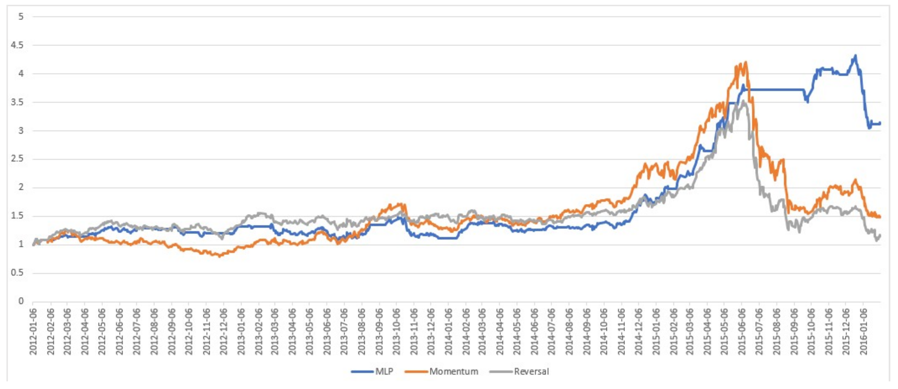
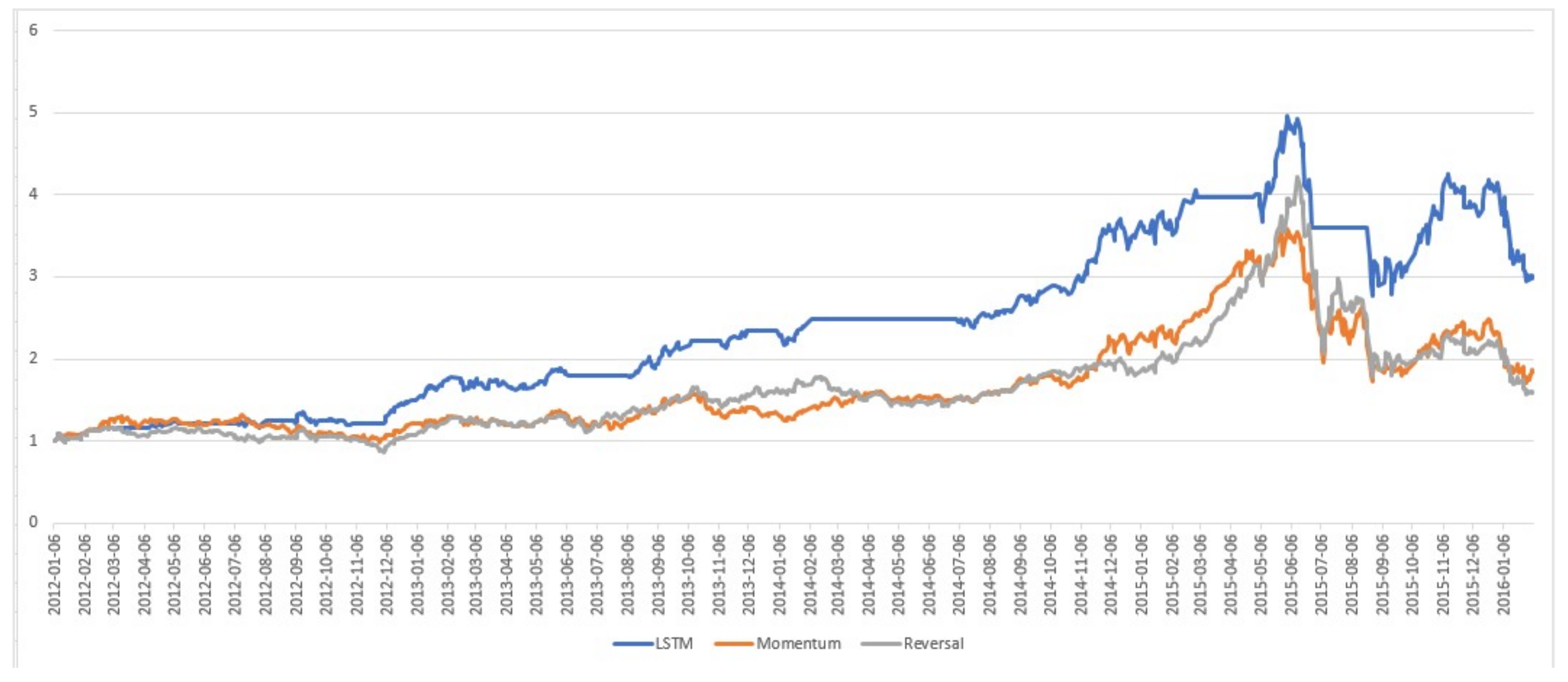
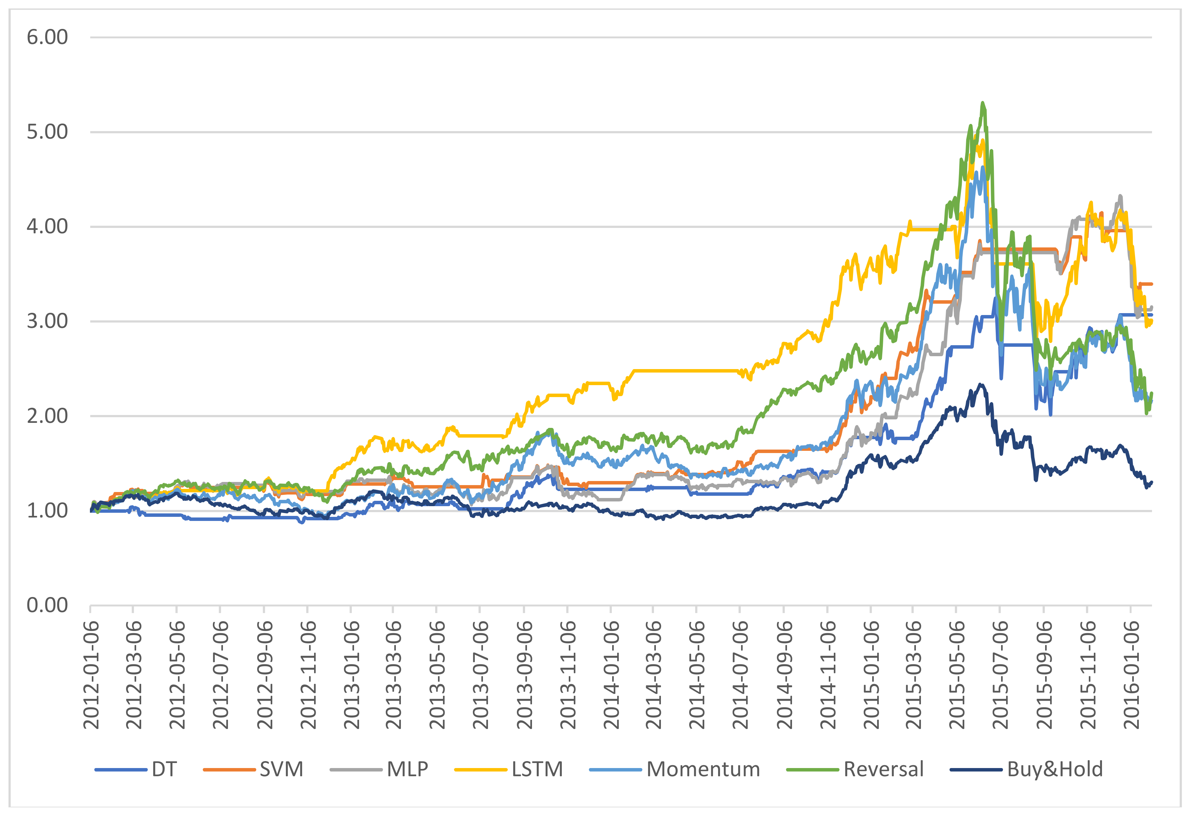
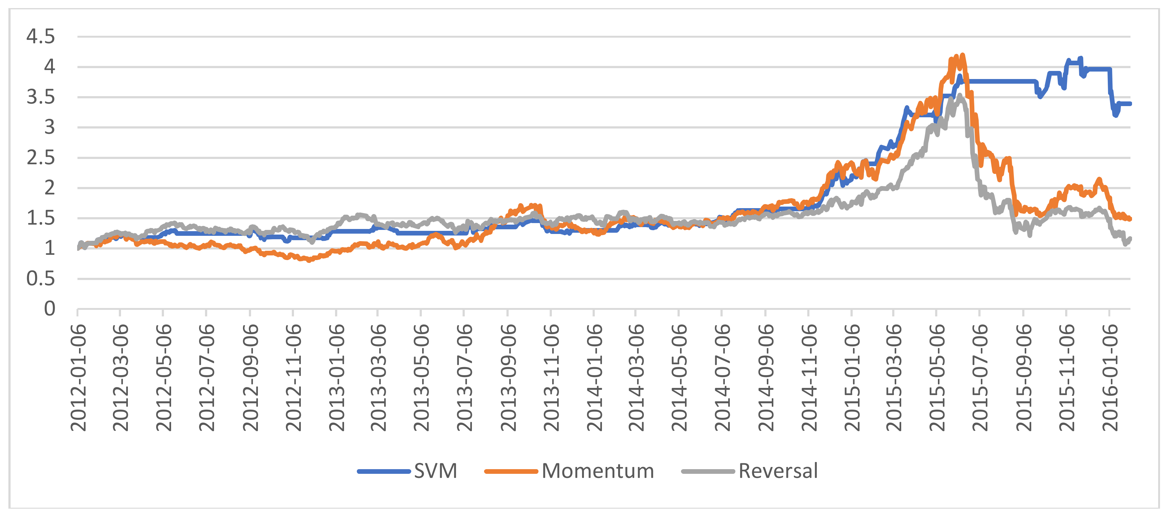
Figure 5, Figure 6, Figure 7 and Figure 8 show the daily Net Asset Value (NAV) curves of portfolios built with the proposed machine learning models, while Figure 9 shows the whole portfolio performance comparison for the best strategies and models.

We identified some interesting phenomena: (1) in the fluctuating market duration, both the best DT and MLP strategies performed poorly. Their NAVs were always below than that of either momentum or reversal strategy, or even both of them, for most of the time when the market trend was not clear. In contrast, the SVM was able to increase its NAV during this period. Furthermore, the LSTM achieved an excellent performance with an increasing NAV. (2) In the bullish market duration, the NAVs of all machine learning models went up dramatically. (3) In the bearish market duration, only the SVM and MLP models were stable and kept their returns. Unfortunately, the performances of LSTM and DT worsened quickly.

These findings suggest we may adopt the LSTM in the fluctuating market, select any machine learning model in the bull market, and change to the SVM to avoid a great loss when a market crash is coming.

6. Conclusions

In summary, this research represents the first attempt to disclose and understand the momentum and reversal effects in the stock market through machine learning techniques. We investigated various machine learning approaches, built corresponding trading strategies, and conducted relevant backtestings.

The experimental results verify that the reversal effect tends to occur in the CSI 300 stock market. By comparing the backtesting results, it has been shown that machine learning approaches were helpful for building more profitable trading strategies. The overall performance beat the benchmark as well as the standalone momentum and reversal trading. Furthermore, we proposed corresponding trading strategies in terms of market states, i.e., LSTM for the fluctuating market state and SVM for the crashing market state.

Up until now, few studies have conducted this type of research. Our research provides a new horizon for the study of momentum and reversal effects on the stock market. It could be beneficial for individual investors building strategies to obtain excess returns from the market. In addition, it is very applicable to algorithmic trading for institutional investors.

Clearly, there is much future work to be carried out. Firstly, the macro-economical indicators and sentiment data extracted from online social networks could be taken into account as features. Secondly, the volatility index (such as VIX for the US stock market, VHSI for Hong Kong stock market) is a powerful tool for measuring and even predicting the current and future volatilities of the market. It would be a pioneer work to combine the volatility indexes with the current work, and this could help the model to analyze and predict the market states more accurately, Thirdly, the selection of observation and holding periods could be investigated more carefully. It would be great if the machine learning model could build an adaptive framework. Furthermore, would definitely be interesting to investigate how the different variants of SVM, such as the fuzzy or twin SVM, or the convolutional neural networks could be adapted for financial forecasting in future studies. Last but not least, it would be worth creating more intelligent and comprehensive models or frameworks ensembling various machine learning models to accommodate complicated market scenarios.