Parameter Estimation of a Class of Neural Systems with Limit Cycles

Abstract

This work addresses parameter estimation of a class of neural systems with limit cycles. An identification model is formulated based on the discretized neural model. To estimate the parameter vector in the identification model, the recursive least-squares and stochastic gradient algorithms including their multi-innovation versions by introducing an innovation vector are proposed. The simulation results of the FitzHugh–Nagumo model indicate that the proposed algorithms perform according to the expected effectiveness.

1. Introduction

1.1. Background

The nervous system is a complex and huge system, composed of a large number of nerve cells. The performance of neurons is closely related to the function of the nervous system. Oscillatory activity is ubiquitous in the nervous system and its synchronous behavior has become an increasing topic in neuroinformatics [1,2]. Although great progress has been made in information coding and understanding nonlinear dynamics of neural oscillator systems in neuroscience and from the system control perspective, there is relatively little research on the modeling and control of neural oscillator systems. In a typical neural system, the measurable state is limited by using voltage clamp technique, while the internal parameters of the system can only be estimated by the measurable state output sequence such as membrane voltage. Sometimes, it is even impossible for biologists to get the modeling information due to various technical difficulties. For example, in the FitzHugh–Nagumo model, the membrane voltage of the neuron is measurable and the model control parameters are unknown, which relies on the parameter identification methods in control theory. In particular, parameter estimation for neural models are used to estimate the uncertain parameters from the available input and output data.

1.2. Parameter Estimation in Neural Model

System parameter estimation has received substantial attention in several decades [3,4,5,6,7]. One reason is its broad application to mechanical systems [8,9], neuron systems [10], communication systems [11], structural systems [12], power systems [13], etc. Existing black-box parameter identification methods for nonlinear systems are simple and universal, but the identification accuracy and convergence of the identification algorithm are not of universal significance. Therefore, accurately identifying the system parameters of the spiking neuron models under finite measurement presents a far more challenging modeling problem. Examples of parameter identification methods for neural models include the time/frequency-domain method [14], maximum likelihood method [15], self-organizing state-space-model approach [16], heuristic optimization method [10], and so on. In [14], a time-domain method and a frequency-domain method are applied to estimate parameters of a neuronal model consisting of a soma coupled to a uniform dendritic cylinder, where the time-domain method is more prone to estimation errors in the cable parameters. Vavoulis et al. [16] presented an adaptive sampling algorithm using the self-organizing state-space model to estimate parameters in a Hodgkin-Huxley-type model of single neurons and to achieve reduced variance of parameter estimates. Mullowney et al. [15] proposed a maximum likelihood methodology for parameter estimation in a leaky integrate-and-fire neuronal model with the only available data being the interspike intervals or the times between firings. In [10], a global heuristic search method using in-vitro and in-vivo electrophysiological data was explored for identification of an Izhikevich-type neuron model.

In spite of these advances, little attention on parameter estimation of the FitzHugh–Nagumo (FHN) model has been received, including Bayesian statistical approaches [17,18], and least-squares algorithms [19,20]. In [17], a Bayesian framework was proposed for drift parameter estimation of the stochastic FHN model. Arnold and Lloyd [18] employed nonlinear filtering for periodic, time-varying parameter estimation, which was illustrated in estimation of the external voltage parameter in the FHN model. In comparison, from the recursive estimation point of view, we perform parameter inference for the FHN model with data generated from the model in this paper. Concha and Garrido [19] presented two methodologies based on the least-squares algorithm to estimate the parameters of the FHN model. The two methods were only suitable for the case with noncontinuous input current stimulus, at the cost of a linear integral filter. Che et al. [20] employed the recursive least-squares algorithm for parameter estimation of the FHN model, which requires the first and second time derivatives of the membrane potential and the input current stimulus being continuously differentiable. It is well known that the stochastic gradient algorithm is a class of important stochastic approximation methods, which have received much attention and have been widely used in different systems, such as Hammerstein systems [21], Wiener systems [22] and sampled systems [23]. Though the stochastic gradient algorithm has a slower convergence rate than the least-squares algorithms, but it requires less computational effort. In this paper, to improve the convergence rate of the stochastic gradient algorithm, we extend the innovation concept in [24] and explore the multiinnovation stochastic gradient algorithm for parameter estimation of the FHN neuron system. The parameterized FHN model in [20] can also be performed by using the proposed multiinnovation recursive least-squares algorithm in this paper and a better accuracy of the parameter estimation will be obtained due to the use of past innovations and repeated available data. However, from the aspect of the computing style, identification algorithms with qualified identification accuracy and convergence are desired for parameter estimation of the neural models. In particular, it seems that little effort has been made toward performing parameter estimation of the FHN model using the stochastic gradient methods.

1.3. Contributions

Inspired by these works, we propose four parameter estimation algorithms for the FHN neuron system with limit cycle and external disturbance. The contributions of this paper include the following:

• We formulate the FHN neuron system as an identification model based on the explicit forward Euler method.
• We propose a recursive least-squares algorithm and a stochastic gradient algorithm to estimate the unknown parameters of the model.
• We extend the innovation concept in [24], and explore the multiinnovation recursive least-squares algorithm and multiinnovation stochastic gradient algorithm for parameter estimation of the FHN neuron system.
• We show that a faster convergence rate and better accuracy can be achieved using the innovation and repeated available data.

1.4. Organization

The organization of the paper is as follows. Section 2 describes the FHN neural model. Section 3 formulates the identification model and presents the parameter estimation problem. The proposed algorithms are given in Section 4, where we estimate the unknown parameters using four different algorithms and summarize corresponding algorithm procedures. Section 5 provides the computational simulations. Finally, we draw some conclusions in Section 6.

2. The Spiking Neuron Model

In this section, we introduce the general spiking neuron models. A conductance-based spiking neuron model is described by

$$\dot{x}\left(t\right)=F\left(x\left(t\right)\right)+Bu\left(t\right)+\xi \left(t\right),$$

(1)

where $x\left(t\right)\in {\mathbb{R}}^n$ is the state which usually consists of the membrane potential, gating variable, recovery variable and adaptation variable; $\xi \left(t\right)\in {\mathbb{R}}^n$ denotes the disturbance in the neuron system; $u\left(t\right)\in \mathbb{R}$ is the external input injected to the neuron; $B\in {\mathbb{R}}^n$ is a constant vector, which is typically taken as $B={[1,\underset{n-1}{\underbrace{0,\cdots ,0}}]}^{\top }$ when the external input acts on the membrane potential.

The system described by (1) is quite general as it includes many spiking neuron models such as the Hodgkin-Huxley model, the Hindmarsh–Rose (HR) model, the FHN model and so on. In this paper, we shall focus on parameter estimation of the FHN model using different identification algorithms, but the proposed approach is applicable to other neuron models in a similar manner. The FHN model in a dimensionless form [25,26] can be written in the form of (1)

$$\left[\begin{array}{c}\dot{v}\left(t\right)\\ \dot{w}\left(t\right)\end{array}\right]=\left[\begin{array}{c}\mu \left(v\right(v+a\left)\right(b-v)-w)+u\left(t\right)\\ c_{1}v-c_{2}w\end{array}\right]+\xi \left(t\right)$$

(2)

where v denotes the voltage potential of the neuron membrane and w denotes the inactivation of the sodium channels; $\xi \in {\mathbb{R}}^2$ denotes the disturbance in the neuron system and is the white noise with zero mean. The parameters $a,b,c_1,c_2,\mu$ are unknown to be estimated later in detail. In this paper, we consider a constant external input $u\left(t\right)\equiv J$ resulting in periodic spiking dynamics and the external input J will also be estimated. Note that when the parameters are specified as $a=0.1$, $b=1$, $c_1=1,c_2=0.5,\mu =100$ and the input current value is taken as $J=0.5$, the neural system from $\left(v\right(0),w(0\left)\right)=(-0.3,0.6)$ without disturbance exhibits periodic spiking dynamics and converge to a limit cycle (see Figure 1).

Figure 1. A limit cycle of the FHN model.

In the real nervous system, the parameters of the spiking neurons are difficult to be measured or determined, the identification of system parameters has always been an important topic in the field of neural computing and system control. Motivated by this, the present work is directed towards developing efficient algorithms to identify the parameters of spiking neuron models.

3. The Identification Model of Spiking Neurons

Usually, the neuron membrane and the inactivation of the sodium channels are discretely sampled in experiment. Hence, let us consider the discretized system of the FHN model using the explicit forward Euler method with step size T as follows

$$\frac{x(k+1)-x\left(k\right)}{T}=f\left(x\left(k\right)\right)+\xi \left(k\right),$$

(3)

where T is the sampling period which is sufficiently small, k represents the $kT$ time instant and

$$f\left(x\left(k\right)\right)=\left[\begin{array}{c}\mu \left(v\left(k\right)\left(v\right(k)+a)(b-v(k\left)\right)-w\left(k\right)\right)+J\\ c_{1}v\left(k\right)-c_{2}w\left(k\right)\end{array}\right].$$

Denote $v_{k,m}:=v(k-m)$, $w_{k,m}:=w(k-m)$ and ${\xi }_{k,m}:=\xi (k-m)$ for $m=1,2,\cdots .$ Then, we have

$$\left[\begin{array}{c}\frac{v\left(k\right)-v(k-1)}{T}\\ \frac{w\left(k\right)-w(k-1)}{T}\end{array}\right]=\left[\begin{array}{c}\mu \left(v_{k,1}(v_{k,1}+a)(b-v_{k,1}\right)-w_{k,1})+J\\ c_1{v}_{k,1}-c_2{w}_{k,1}\end{array}\right]+{\xi }_{k,1}$$

(4)

Define $y\left(k\right)={[y_1\left(k\right),y_2\left(k\right)]}^{\top }$, $y_1\left(k\right)=(v\left(k\right)-v(k-1))/T,$ $y_2\left(k\right)=(w\left(k\right)-w(k-1))/T,$ $\theta \left(k\right)={\left[\begin{array}{cccccc}\mu & (a+b)\mu & ab\mu & J& c_1& c_2\end{array}\right]}^{\top }$ and

$$\varphi \left(k\right)={\left[\begin{array}{cccccc}-v_{k,1}^3-w_{k,1}& v_{k,1}^2& -v_{k,1}& 1& 0& 0\\ 0& 0& 0& 0& v_{k,1}& -w_{k,1}\end{array}\right]}^{\top }.$$

Therefore, Equation (4) can be rewritten as

$$y\left(k\right)={\varphi }^{\top }\left(k\right)\theta \left(k\right)+{\xi }_{k,1}$$

(5)

which is called as the identification model. Apparently, to estimate the parameters $a,b,\mu ,J,c_1,c_2$, it is equivalent to estimate the parameter vector $\theta$.

4. Parameter Estimation of the Spiking Neurons

4.1. Least-Squares Estimation Algorithms

To estimate the parameters $\theta$, let us consider the cost function

$$\mathbb{J}\left(\theta \right)=\sum _{k=1}^{L_d}\sum _{i=1}^2{(y_i\left(k\right)-{\varphi }_i^{\top }\left(k\right)\theta )}^2,$$

where $L_d$ denotes the data length. Using the least-squares principle to solve the optimization problem, we explore the following recursive least-squares (RLS) parameter estimation formulas [3,27] to estimate the parameter vector $\theta \left(k\right)$.

$$\begin{array}{c}\hfill \left\{\begin{array}{ccc}\widehat{\theta }\left(k\right)& =\hfill & \widehat{\theta }(k-1)+L\left(k\right)\epsilon \left(k\right),\hfill \\ \epsilon \left(k\right)& =\hfill & \left[\begin{array}{c}{y}_1\left(k\right)-{\varphi }_1^{\top }\left(k\right)\widehat{\theta }(k-1)\\ y_2\left(k\right)-{\varphi }_2^{\top }\left(k\right)\widehat{\theta }(k-1)\end{array}\right],\hfill \\ L\left(k\right)& =\hfill & P(k-1)\varphi \left(k\right){\left[\lambda +{\varphi }^{\top }\left(k\right)P(k-1)\varphi \left(k\right)\right]}^{-1},\hfill \\ P\left(k\right)& =\hfill & (I-L\left(k\right){\varphi }^{\top }\left(k\right))P(k-1),\hfill \end{array}\right.\end{array}$$

(6)

where $\lambda \in (0,1]$ is the forgotten factor, $P\left(k\right)\in {\mathbb{R}}^{\tilde{n}\times \tilde{n}}$ is the vector of adjustment gains, $\tilde{n}=6$, $P\left(0\right)=p_{0}I$, and $p_0$ is a large positive number.

To initialize the RLS algorithm, the initial value $\widehat{\theta }\left(0\right)$ is generally taken to be a zero vector or a small real vector, e.g., $\widehat{\theta }\left(0\right)={10}^{-6}{\mathbf{1}}_{\tilde{n}}$ with ${\mathbf{1}}_{\tilde{n}}$ being an $\tilde{n}$-dimensional column vector whose elements are 1. Now, the RLS parameter estimation algorithm for the spiking neuron model is summarized in Algorithm 1.

Algorithm 1 RLS algorithm

(1) Discretize the FHN model based on the explicit forward Euler method with step size T. (2) Initialization: set the forgotten factor $\lambda \in (0,1]$ and let $k=1,$$\widehat{\theta }\left(0\right)={\mathbf{1}}_{\tilde{n}}/p_0$, $P\left(0\right)=p_{0}I$, $p_0={10}^6$. (3) Collect the measurement state data and determine a data length $L_d$. Then, form the output data $y\left(k\right)$ and the information vector $\varphi \left(k\right)$. (4) Compute $L\left(k\right)$ and $P\left(k\right)$ by $$L\left(k\right)=\frac{P(k-1)\varphi \left(k\right)}{\lambda +{\varphi }^{\top }\left(k\right)P(k-1)\varphi \left(k\right)},P\left(k\right)=(I-L\left(k\right){\varphi }^{\top }\left(k\right))P(k-1),$$ respectively. (5) Update the estimate $\widehat{\theta }\left(k\right)$ by $\widehat{\theta }\left(k\right)=\widehat{\theta }(k-1)+L\left(k\right)\epsilon \left(k\right),$ where $$\epsilon \left(k\right)=\left[\begin{array}{c}{y}_1\left(k\right)-{\varphi }_1^{\top }\left(k\right)\widehat{\theta }(k-1)\\ y_2\left(k\right)-{\varphi }_2^{\top }\left(k\right)\widehat{\theta }(k-1)\end{array}\right].$$ (6) If $k<L_d$, increase k by 1 and go to step (3); otherwise, stop the procedure and output the estimate $\widehat{\theta }\left(L_d\right)$ of the parameter vector $\theta$.

To obtain better estimation accuracy, we modify the algorithm (6) and apply a multiinnovation recursive least-squares (MIRLS) parameter estimation algorithm [7] for (5) by introducing an innovation length p. By defining the information matrix $\Phi (p,k)$ and stacked output vector $Y(p,k)$ as

$$Y(p,k)={[y^{\top }\left(k\right),y^{\top }(k-1),\cdots ,y^{\top }(k-p+1)]}^{\top }\in {\mathbb{R}}^{2p},$$

(7)

$$\Phi (p,k)={[{\varphi }^{\top }\left(k\right),{\varphi }^{\top }(k-1),\cdots ,{\varphi }^{\top }(k-p+1)]}^{\top }\in {\mathbb{R}}^{6\times 2p},$$

(8)

the innovation vector $\mathcal{E}(p,k)$ can be expressed as

$$\mathcal{E}\left(k\right)=Y(p,k)-{\Phi }^{\top }(p,k)\widehat{\theta }(k-1).$$

From here, we present the following MIRLS iterative formulas

$$\begin{array}{c}\hfill \left\{\begin{array}{ccc}\widehat{\theta }\left(k\right)& =\hfill & \widehat{\theta }(k-1)+L\left(k\right)\mathcal{E}\left(k\right),\hfill \\ \mathcal{E}\left(k\right)& =\hfill & Y(p,k)-{\Phi }^{\top }(p,k)\widehat{\theta }(k-1),\hfill \\ L\left(k\right)& =\hfill & P(k-1)\Phi (p,k){\left[\lambda +{\Phi }^{\top }(p,k)P(k-1)\Phi (p,k)\right]}^{-1},\hfill \\ P\left(k\right)& =\hfill & (I-L\left(k\right){\Phi }^{\top }(p,k))P(k-1).\hfill \end{array}\right.\end{array}$$

(9)

The MIRLS parameter estimation algorithm for the FHN model is summarized in Algorithm 2.

Algorithm 2 MIRLS algorithm

(1) Discretize the FHN model based on the explicit forward Euler method with step size T. (2) Initialization: set the forgotten factor $\lambda \in (0,1]$ and let $k=1,$$\widehat{\theta }\left(0\right)={\mathbf{1}}_{\tilde{n}}/p_0$, $P\left(0\right)=p_{0}I$, $p_0={10}^6$. (3) Collect the measurement state data and determine a data length $L_d$. Then, form the output data $y\left(k\right)$ and the information vector $\varphi \left(k\right)$. (4) Given an innovation length p, form $Y(p,k)$ by (7) and $\Phi (p,k)$ by (8). (5) Compute $L\left(k\right)$ and $P\left(k\right)$ by $$L\left(k\right)=\frac{P(k-1)\Phi (p,k)}{\lambda +{\Phi }^{\top }(p,k)P(k-1)\Phi (p,k)}$$ and $$P\left(k\right)=(I-L\left(k\right){\Phi }^{\top }(p,k))P(k-1),$$ respectively. (6) Update the estimate $\widehat{\theta }\left(k\right)$ by $\widehat{\theta }\left(k\right)=\widehat{\theta }(k-1)+L\left(k\right)\mathcal{E}\left(k\right),$ where $$\mathcal{E}\left(k\right)=Y(p,k)-{\Phi }^{\top }(p,k)\widehat{\theta }(k-1).$$ (7) If $k<L_d$, increase k by 1 and go to step (3); otherwise, stop the procedure and output the estimate $\widehat{\theta }\left(L_d\right)$ of the parameter vector $\theta$.

4.2. Stochastic Gradient Estimation Algorithms

Let ${\parallel X\parallel }^2:=\mathrm{tr}\left[X{X}^{\top }\right]$ denote the norm of the matrix $X.$ For the model (5), we present the following stochastic gradient (SG) parameter estimation formulas to estimate the parameter vector $\theta \left(k\right)$

$$\begin{array}{c}\hfill \left\{\begin{array}{ccc}\widehat{\theta }\left(k\right)& =\hfill & \widehat{\theta }(k-1)+\frac{1}{r\left(k\right)}\varphi \left(k\right)\epsilon \left(t\right),\hfill \\ \epsilon \left(t\right)& =\hfill & \left[\begin{array}{c}{y}_1\left(k\right)-{\varphi }_1^{\top }\left(k\right)\widehat{\theta }(k-1)\\ y_2\left(k\right)-{\varphi }_2^{\top }\left(k\right)\widehat{\theta }(k-1)\end{array}\right],\hfill \\ r\left(k\right)& =\hfill & \alpha r(k-1)+{\parallel \varphi \left(k\right)\parallel }^2,r\left(0\right)=1,\hfill \end{array}\right.\end{array}$$

(10)

where $\alpha$ is the forgotten factor. Note that a smaller $\alpha$ results in a faster convergence but the price we paid is a large parameter fluctuation. In this paper, since the SG algorithm converges slowly in parameter estimation of the FHN neuron, we choose a moderate $\alpha =0.8$.

The SG parameter estimation algorithm for the spiking neuron model is summarized in Algorithm 3.

Algorithm 3 SG algorithm

(1) Discretize the FHN model based on the explicit forward Euler method with step size T. (2) Initialization: set a small forgotten factor $\alpha \in (0,1]$ and let $k=1,$$\widehat{\theta }\left(0\right)={\mathbf{1}}_{\tilde{n}}/p_0$, $r\left(0\right)=1$, $p_0={10}^6$. (3) Collect the measurement state data and determine a data length $L_d$. Then, form the output data $y\left(k\right)$ and the information vector $\varphi \left(k\right)$. (4) Compute $r\left(k\right)$ by $r\left(k\right)=\alpha r(k-1)+{\parallel \varphi \left(k\right)\parallel }^2.$ (5) Update the estimate $\widehat{\theta }\left(k\right)$ by $\widehat{\theta }\left(k\right)=\widehat{\theta }(k-1)+\varphi \left(k\right)\epsilon \left(t\right)/r\left(k\right),$ where $\epsilon \left(t\right)=\left[\begin{array}{c}{y}_1\left(k\right)-{\varphi }_1^{\top }\left(k\right)\widehat{\theta }(k-1)\\ y_2\left(k\right)-{\varphi }_2^{\top }\left(k\right)\widehat{\theta }(k-1)\end{array}\right].$ (6) If $k=L_d/2$, reset a large forgotten factor $\alpha \in (0,1]$ and go to step (7); otherwise, go to step (7). (7) If $k<L_d$, increase k by 1 and go to step (3); otherwise, stop the procedure and output the estimate $\widehat{\theta }\left(L_d\right)$ of the parameter vector $\theta$.

Similarly, to obtain better estimation accuracy, we can derive multiinnovation stochastic gradient (MISG) parameter estimation formulas [28] using the $Y(p,k)$ and $\Phi (p,k)$ in Section 4.1 as follows

$$\begin{array}{c}\hfill \left\{\begin{array}{ccc}\widehat{\theta }\left(k\right)& =\hfill & \widehat{\theta }(k-1)+\Phi (p,k)\mathcal{E}\left(t\right)/r\left(k\right),\hfill \\ \mathcal{E}\left(k\right)& =\hfill & Y(p,k)-{\Phi }^{\top }(p,k)\widehat{\theta }(k-1),\hfill \\ r\left(k\right)& =\hfill & \alpha r(k-1)+{\parallel \Phi (p,k)\parallel }^2,r\left(0\right)=1.\hfill \end{array}\right.\end{array}$$

(11)

Comparing with the SG algorithm in (10) using only the current data, the innovation $\Phi$ in (11) uses not only the current innovation, but also the past innovations, which thus can improve the convergence rates compared with the SG algorithm. Moreover, the available data are repeatedly used in the MISG algorithm, and such a treatment can enhance accuracy of the parameter estimation [24]. The MISG parameter estimation algorithm for the FHN model is summarized in Algorithm 4.

Algorithm 4 MISG algorithm

(1) Discretize the FHN model based on the explicit forward Euler method with step size T. (2) Initialization: set a small forgotten factor $\alpha \in (0,1]$ and let $k=1,$$\widehat{\theta }\left(0\right)={\mathbf{1}}_{\tilde{n}}/p_0$, $r\left(0\right)=1$, $p_0={10}^6$. (3) Collect the measurement state data and determine a data length $L_d$. Then, form the output data $y\left(k\right)$ and the information vector $\varphi \left(k\right)$. (4) Given an innovation length p, form $Y(p,k)$ by (7) and $\Phi (p,k)$ by (8). (5) Compute $r\left(k\right)$ by $r\left(k\right)=\alpha r(k-1)+{\parallel \Phi (p,k)\parallel }^2.$ (6) Update the estimate $\widehat{\theta }\left(k\right)$ by $\widehat{\theta }\left(k\right)=\widehat{\theta }(k-1)+\Phi (p,k)\mathcal{E}\left(t\right)/r\left(k\right)$, $\mathcal{E}\left(k\right)=Y(p,k)-{\Phi }^{\top }(p,k)\widehat{\theta }(k-1).$ (7) If $k=L_d/2$, reset a large forgotten factor $\alpha \in (0,1]$ and go to step (8); otherwise, go to step (8). (8) If $k<L_d$, increase k by 1 and go to step (3); otherwise, stop the procedure and output the estimate $\widehat{\theta }\left(L_d\right)$ of the parameter vector $\theta$.

5. Simulations

For purpose of illustration, we consider the FHN model [25,26] described in the dimensionless form (2). In simulation, the parameters are taken as $a=0.1,b=1,c_1=1,c_2=0.5,\mu =100$ and $J=0.5.$ The FHN model is firstly discretized based on the explicit forward Euler method with step size $T=10\mathrm{ms}$. Then, consider the initial value $v\left(0\right)=-0.3,w\left(0\right)=0.6$, and perform the simulations based on the identification algorithms in Section 4. Taking the data length $L_d=20,000$, the forgotten factor $\lambda$ is chosen as $0.99$ for RLS and MIRLS algorithms. For both SG and MISG algorithms, we take the forgotten factor $\alpha =0.8$. To compare the estimation performance of the RLS, SG, MIRLS and MISG algorithms, apply these four algorithms to estimate the parameter vector $\theta$ of the neuron system, respectively. Note that, when $p=1,$ the MIRLS algorithm reduces to the RLS algorithm and the MISG algorithm reduces to the SG algorithm. For the MIRLS and MISG algorithms, two cases with different innovation lengths $p=3$ and $p=5$ are considered, respectively. To quantify the estimation accuracy and clearly compare the performance of the RLS, SG, MIRLS and MISG algorithms, we consider two different noise levels, i.e., ${\sigma }^2=0.2^2$ and ${\sigma }^2=0.5^2$. The parameter estimates and their errors are shown in Table 1, Table 2, Table 3 and Table 4 with different noise variances. The estimation errors $\delta$ versus k are shown in Figure 2 and Figure 3, where $\delta :=\parallel \widehat{\theta }-\theta \parallel /\parallel \theta \parallel$.

Table 1. The RLS estimates and errors.

${\mathit{\sigma }}^2$	k	$\mathit{\mu }$	$(\mathit{a}+\mathit{b})\mathit{\mu }$	$\mathit{ab}\mathit{\mu }$	J	${\mathit{c}}_1$	${\mathit{c}}_2$	$\mathit{\delta }(\%)$
	10	3.7906	−0.7233	0.6077	2.9444	2.6491	0.3230	98.2022
	20	1.6180	4.6890	−6.8895	2.7357	1.8070	0.5639	97.0998
$0.2^2$	50	94.7731	102.8236	8.3295	47.5574	0.9996	0.6066	5.9548
	100	99.1037	108.8017	9.7432	49.5408	1.0207	0.5576	1.0100
	150	99.2001	108.8906	9.7232	49.5928	1.0401	0.5390	0.9256
	200	99.5227	109.3771	9.8946	49.7620	1.0404	0.5346	0.5272
	10	19.0174	−2.3066	7.1256	10.3718	4.2456	0.4154	91.6760
	20	11.4943	28.0891	−11.5647	8.2026	2.0516	0.9504	82.3618
$0.5^2$	50	93.5511	100.3815	7.4373	47.0843	1.2176	0.9968	7.7788
	100	98.8246	108.3058	9.5814	49.3799	1.0948	0.6696	1.4012
	150	98.9660	108.4155	9.5199	49.4549	1.1355	0.6290	1.2950
	200	99.7218	109.5163	9.8858	49.8592	1.1210	0.5971	0.3861
True values		100.0000	110.0000	10.0000	50.0000	1.0000	0.5000

Table 2. The MIRLS estimates and errors ($p=3$).

${\mathit{\sigma }}^2$	k	$\mathit{\mu }$	$(\mathit{a}+\mathit{b})\mathit{\mu }$	$\mathit{ab}\mathit{\mu }$	J	${\mathit{c}}_1$	${\mathit{c}}_2$	$\mathit{\delta }(\%)$
	10	7.9850	−1.6092	2.5997	4.8664	2.4115	0.3541	96.5310
	20	3.4710	8.9666	−7.0001	3.6340	1.7240	0.5638	94.2987
$0.2^2$	50	98.1459	107.4963	9.4579	49.1372	0.9894	0.6051	2.0867
	100	99.6327	109.4124	9.8139	49.8019	1.0195	0.5559	0.4751
	150	99.5767	109.3555	9.7988	49.7747	1.0364	0.5407	0.5280
	200	99.7563	109.6468	9.9260	49.8776	1.0393	0.5327	0.2896
	10	33.4907	−4.5706	13.6947	17.0438	3.7755	0.4402	86.9092
	20	24.8108	41.9383	−8.4833	14.4792	1.9920	0.9177	69.3805
$0.5^2$	50	96.1344	104.1168	8.4045	48.2817	1.1906	0.9819	4.7325
	100	99.3021	108.8667	9.6535	49.6153	1.0919	0.6652	0.9166
	150	99.3244	108.8691	9.6029	49.6278	1.1276	0.6338	0.9145
	200	99.9346	109.7613	9.9147	49.9651	1.1189	0.5926	0.1935
True values		100.0000	110.0000	10.0000	50.0000	1.0000	0.5000

Table 3. The SG estimates and errors.

${\mathit{\sigma }}^2$	k	$\mathit{\mu }$	$(\mathit{a}+\mathit{b})\mathit{\mu }$	$\mathit{ab}\mathit{\mu }$	J	${\mathit{c}}_1$	${\mathit{c}}_2$	$\mathit{\delta }(\%)$
	500	13.3084	−7.8497	13.6492	11.1506	1.0467	0.4382	96.3408
	1000	21.9925	−4.8275	9.1816	21.6546	1.0218	0.5516	90.1498
$0.2^2$	5000	61.4462	38.2353	2.5148	31.3570	1.0511	0.5234	53.3865
	10,000	79.7290	72.4560	5.9073	40.7280	1.0606	0.5298	27.9030
	15,000	88.3858	90.8851	7.0928	46.6020	1.0202	0.5696	14.5130
	20,000	94.5236	99.8808	8.9198	47.4423	0.9398	0.3133	7.5321
	500	15.7472	−7.8692	14.3078	8.5323	1.0953	0.3400	95.9265
	1000	22.1267	−4.0507	8.4011	23.2820	1.0782	0.6592	89.5044
$0.5^2$	5000	61.7189	39.9100	1.8494	34.0418	1.1217	0.5866	52.0776
	10,000	81.1552	73.8568	5.7945	40.9238	0.8981	0.5475	26.7046
	15,000	90.2873	91.2729	7.7195	45.1400	1.0227	0.6214	13.8507
	20,000	95.0617	100.5981	8.9675	47.9177	0.8727	0.0131	6.9244
True values		100.0000	110.0000	10.0000	50.0000	1.0000	0.5000

Table 4. The MISG estimates and errors ($p=3$).

${\mathit{\sigma }}^2$	k	$\mathit{\mu }$	$(\mathit{a}+\mathit{b})\mathit{\mu }$	$\mathit{ab}\mathit{\mu }$	J	${\mathit{c}}_1$	${\mathit{c}}_2$	$\mathit{\delta }(\%)$
	500	19.1634	−11.8220	23.2437	16.5106	1.1374	0.4206	95.8047
	1000	35.0060	−8.8759	18.5691	37.0688	1.0426	0.5921	86.7670
$0.2^2$	5000	85.1399	57.0311	−0.6404	42.6241	1.0992	0.5409	35.9599
	10,000	94.1694	90.4475	6.3213	47.8311	1.0994	0.5577	13.2635
	15,000	97.3389	103.1461	8.3135	49.9311	1.0338	0.6045	4.8003
	20,000	99.1619	107.5047	9.5947	49.7100	0.9374	0.2108	1.7150
	500	23.1916	−11.9815	24.6474	12.4417	1.2785	0.2591	95.2371
	1000	35.3666	−7.5615	17.1582	39.9121	1.1419	0.7780	85.7224
$0.5^2$	5000	85.5678	59.2415	−0.6955	44.1461	1.2350	0.6827	34.4612
	10,000	95.2375	91.8121	6.4314	47.7921	0.9014	0.6650	12.2575
	15,000	98.4425	103.4602	8.5951	49.2526	1.0869	0.7208	4.3983
	20,000	99.6694	108.1012	9.7009	50.1496	0.9396	−0.2527	1.3341
True values		100.0000	110.0000	10.0000	50.0000	1.0000	0.5000

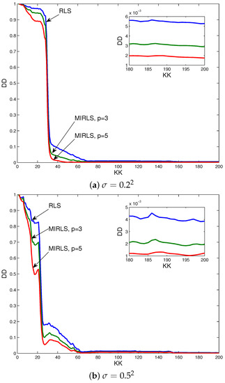
Figure 2. Parameter estimation errors $\delta$ versus k using RLS and MIRLS.

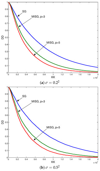
Figure 3. Parameter estimation errors $\delta$ versus k using SG and MISG.

From Table 1 and Table 2, it is seen that both the RLS and MIRLS algorithms have a fast convergence rate and a high estimation accuracy, which can also be observed from Figure 2 and Figure 3. On the other hand, by using the SG and MISG algorithms, it is shown in Table 3 and Table 4 that it requires a data length around $L_d=20,000$ to achieve an acceptable estimation accuracy. Though not shown in table, the MIRLS algorithm with $p=5$ enjoys the most accurate parameter estimate and the fastest convergence rate. From Figure 2 and Figure 3, we can see that for the same batch of data, compared with the RLS algorithm, the SG algorithm extracts less information from the measured data and uses information inefficiently, which results in a much slower convergence. Hence, to show the effect clearly, the results by the RLS and SG algorithms are shown in two figures, respectively. Meanwhile, from Figure 2, it can be found that due to the high efficiency of the RLS algorithm, the MIRLS algorithm has limited improvement potential for the accuracy of parameter estimation. However, the computation efficiency of the MIRLS algorithm will be revealed in the case of data missing, which remains our future work. From Figure 3, it is clear that the MISG algorithm has a faster convergence rate than the SG algorithm or the MISG algorithm with $p=1$ and the MISG estimates with $p=3$ and $p=5$ have higher accuracy than the SG estimates. In fact, the parameter estimation errors by the MISG algorithm become smaller and smaller as the innovation length p increases.

6. Conclusions

In this paper, we have addressed the parameter estimation problem of the FHN neuron model with limit cycles by utilizing the RLS, MIRLS, SG and MISG algorithms. The MIRLS and MISG identification algorithms, which take into the account history innovations, have been applied to improve the accuracy of identification. The framework using the algorithms here could serve as a template for performing parameter inference on more complex neuronal models. Finally, simulation results have been provided to corroborate the effectiveness of the proposed algorithms.

References

- Buzsaki, G.; Draguhn, A. Neuronal oscillations in cortical networks. Science 2004, 304, 1926–1929. [Google Scholar] [CrossRef] [PubMed]
- Singer, W. Neuronal synchrony: A versitile code for the definition of relations. Neuron 1999, 24, 49–65. [Google Scholar] [CrossRef]
- Ljung, L. System Identification: Theory for the User; Prentice-Hall: Englewood Cliffs, NJ, USA, 1987. [Google Scholar]
- Ljung, L. Perspectives on system identification. Annu. Rev. Control 2010, 34, 1–12. [Google Scholar] [CrossRef]
- Juang, J.N.; Phan, M.Q. Identification and Control of Mechanical Systems; Cambridge University Press: Cambridge, UK, 2001. [Google Scholar]
- Moonen, M.; Ramos, J. A subspace algorithm for balanced state space system identification. IEEE Trans. Autom. Control 1993, 38, 1727–1729. [Google Scholar] [CrossRef]
- Ding, F. System Identification-New Theory and Methods; Science Press: Beijing, China, 2013. [Google Scholar]
- Pappalardo, C.M.; Guida, D. A time-domain system identification numerical procedure for obtaining linear dynamical models of multibody mechanical systems. Archiv. Appl. Mech. 2018, 88, 1325–1347. [Google Scholar] [CrossRef]
- Pappalardo, C.M.; Guida, D. System identification algorithm for computing the modal parameters of linear mechanical systems. Machines 2018, 6, 1–20. [Google Scholar]
- Lynch, E.P.; Houghton, C.J. Parameter estimation of neuron models using in-vitro and in-vivo electrophysiological data. Front. Neuroinf. 2015, 9, 10. [Google Scholar] [CrossRef] [PubMed]
- Duan, C.; Zhan, Y. The response of a linear monostable system and its application in parameters estimation for PSK signals. Phys. Lett. A 2016, 380, 1358–1362. [Google Scholar] [CrossRef]
- Pappalardo, C.M.; Guida, D. System identification and experimental modal analysis of a frame structure. Eng. Lett. 2018, 26, 56–68. [Google Scholar]
- Kenné, G.; Ahmed-Ali, T.; Lamnabhi-Lagarrigue, F.; Arzandé, A. Nonlinear systems time-varying parameter estimation: application to induction motors. Electr. Power Syst. Res. 2008, 78, 1881–1888. [Google Scholar] [CrossRef]
- Tabak, J.; Murphey, R.; Moore, L.E. Parameter estimation methods for single neuron models. J. Comput. Neurosci. 2000, 9, 215–236. [Google Scholar] [CrossRef] [PubMed]
- Mullowney, P.; Iyengar, S. Parameter estimation for a leaky integrate-and-fire neuronal model from ISI data. J. Comput. Neurosci. 2008, 24, 179–194. [Google Scholar] [CrossRef] [PubMed]
- Vavoulis, D.V.; Straub, V.A.; Aston, J.A.D.; Feng, F. A self-organizing state-space-model approach for parameter estimation in Hodgkin-Huxley-type models of single neurons. PLoS Comput. Biol. 2012, 8, e1002401. [Google Scholar] [CrossRef] [PubMed]
- Jensen, A.; Ditlevsen, S.; Kessler, M.; Papaspiliopoulos, O. Markov chain Monte Carlo approach to parameter estimation in the FitzHugh–Nagumo model. Phys. Rev. E 2012, 86, 041114. [Google Scholar] [CrossRef] [PubMed]
- Arnold, A.; Lloyd, A.L. An approach to periodic, time-varying parameter estimation using nonlinear filtering. Inverse Probl. 2018, 34, 105005. [Google Scholar] [CrossRef]
- Concha, A.; Carrido, R. Parameter estimation of the FitHugh–Nagumo neuron model using integrals over finite time periods. J. Comput. Nonlinear Dyn. 2015, 10, 021023. [Google Scholar] [CrossRef]
- Che, Y.; Geng, L.; Han, C.; Cui, S.; Wang, J. Parameter estimation of the FitzHugh–Nagumo model using noisy measurements for membrane potential. Chaos 2012, 22, 023139. [Google Scholar] [CrossRef] [PubMed]
- Ding, F. Hierarchical multi-innovation stochastic gradient algorithm for Hammerstein nonlinear system modeling. Appl. Math. Model. 2013, 37, 1694–1704. [Google Scholar] [CrossRef]
- Li, J.; Hua, C.; Tang, Y.; Guan, X. Stochastic gradient with changing forgetting factor-based parameter identification for Wiener systems. Appl. Math. Lett. 2014, 33, 40–45. [Google Scholar] [CrossRef]
- Chen, J.; Lv, L.; Ding, R. Multi-innovation stochastic gradient algorithms for dual-rate sampled systems with preload nonlinearity. Appl. Math. Lett. 2013, 26, 124–129. [Google Scholar] [CrossRef]
- Ding, F.; Chen, T. Performance analysis of multi-innovation gradient type identification methods. Automatica 2007, 43, 1–14. [Google Scholar] [CrossRef]
- Keener, J.; Sneyd, J. Mathematical Physiology; Springer: New York, NY, USA, 2009; pp. 1–47. [Google Scholar]
- Danzl, P.; Hespanha, J.; Moehlis, J. Event-based minimum-time control of oscillatory neuron models: phase randomization, maximal spike rate increase, and desynchronization. Biol. Cybern. 2009, 101, 387–399. [Google Scholar] [CrossRef] [PubMed]
- Ding, F.; Wang, Y.J.; Dai, J.Y.; Li, Q.S.; Chen, Q.J. A recursive least squares parameter estimation algorithm for output nonlinear autoregressive systems using the input-output data filtering. J. Franklin Inst. 2017, 354, 6938–6955. [Google Scholar] [CrossRef]
- Xu, L.; Ding, F.; Gu, Y.; Alsaedi, A.; Hayat, T. A multi-innovation state and parameter estimation algorithm for a state space system with d-step state-delay. Signal Process. 2017, 140, 97–103. [Google Scholar] [CrossRef]
© 2018 by the authors. Licensee MDPI, Basel, Switzerland. This article is an open access article distributed under the terms and conditions of the Creative Commons Attribution (CC BY) license (http://creativecommons.org/licenses/by/4.0/).