Intelligent Dynamic Backlash Agent: A Trading Strategy Based on the Directional Change Framework

Abstract
1. Introduction
2. Directional Changes: An Introduction
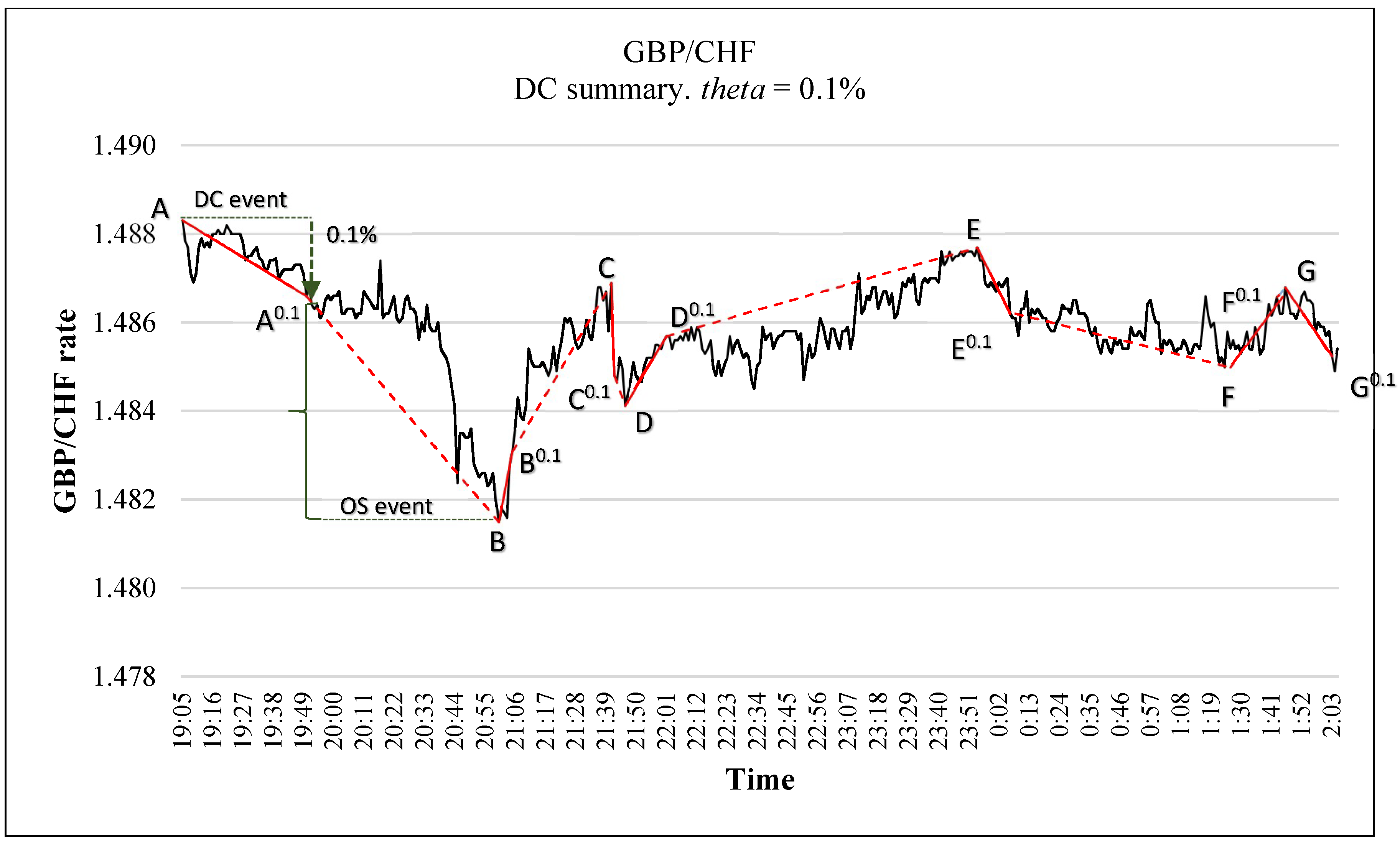
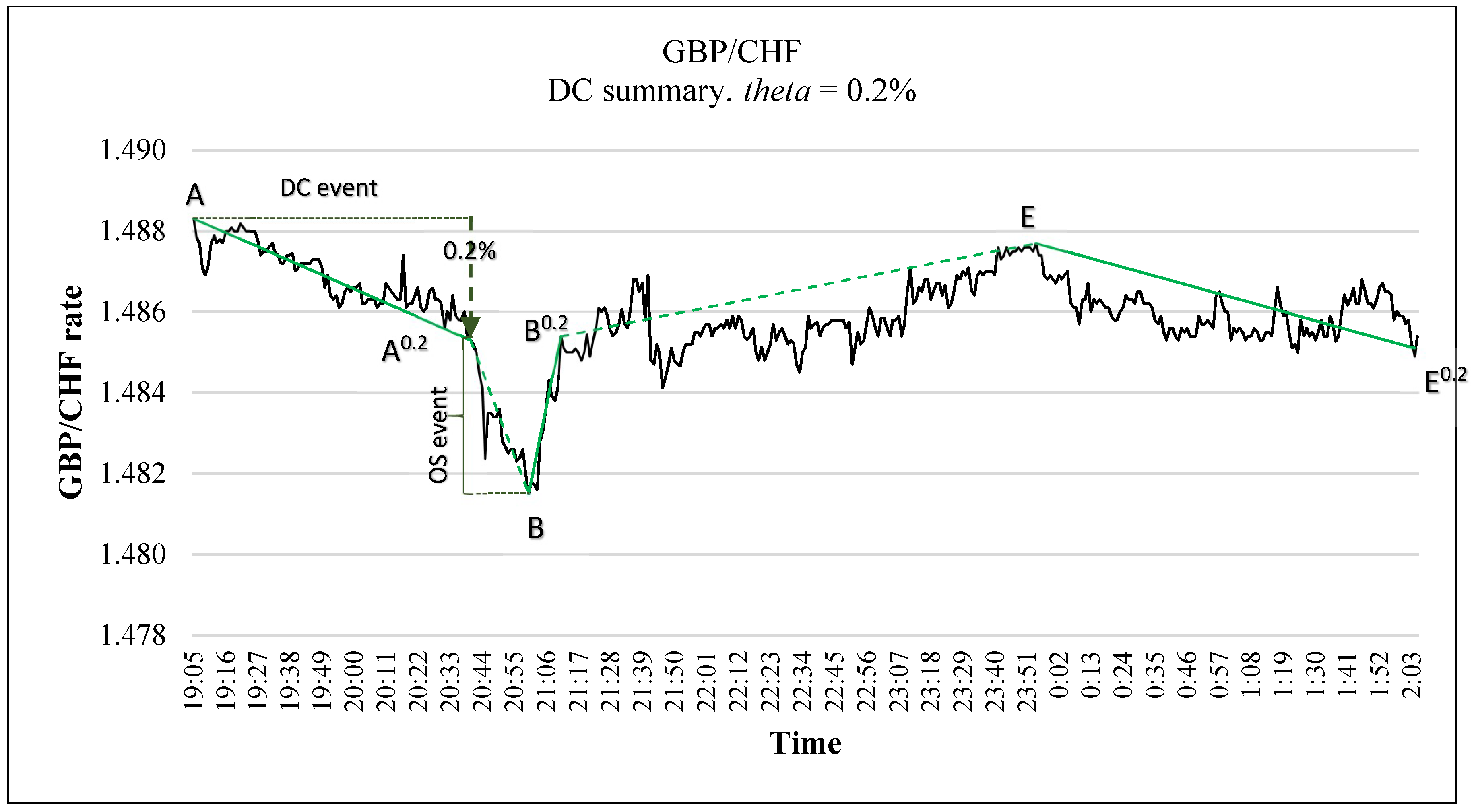
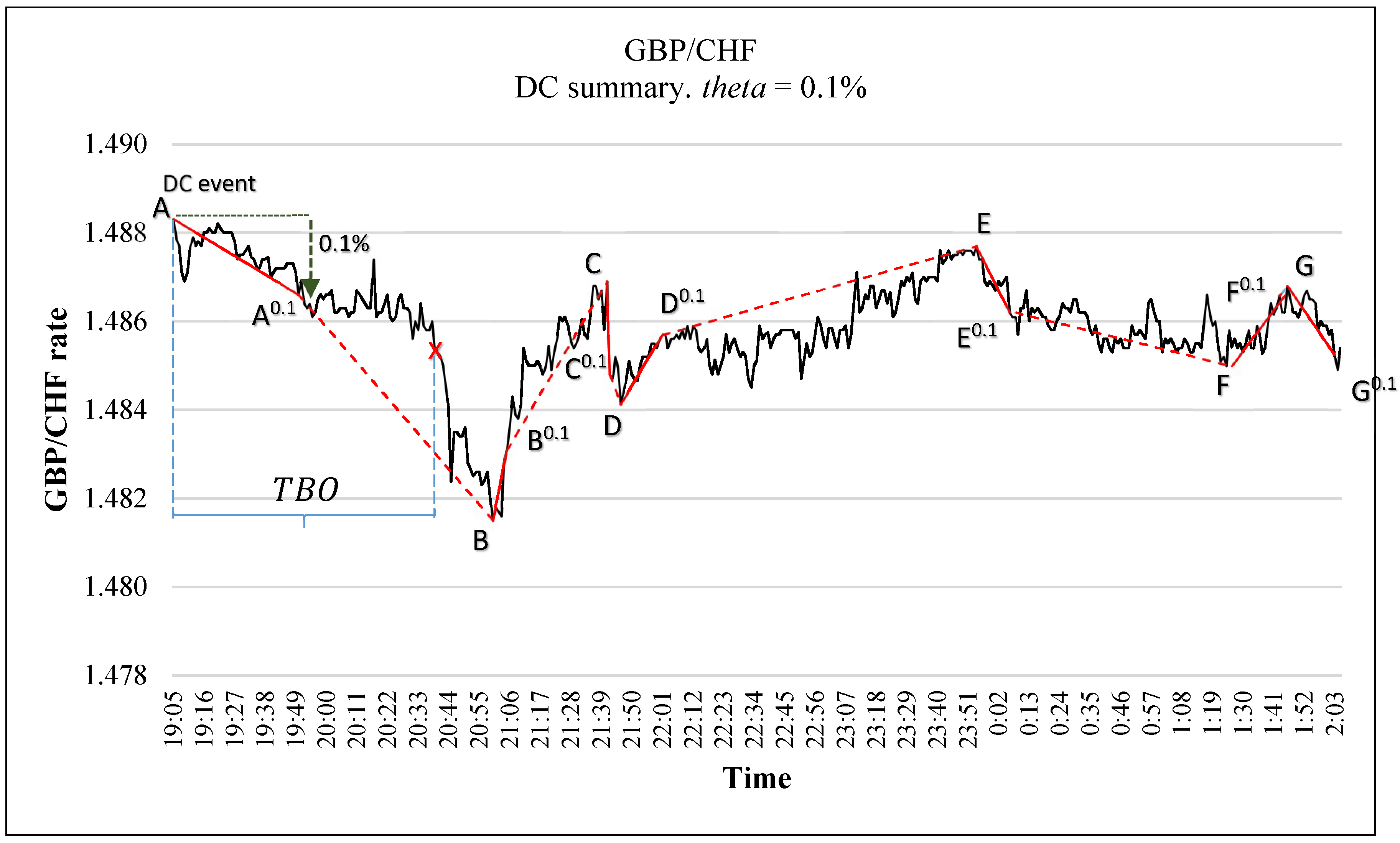
- Step 1: If the market is currently in a downtrend, let denotes the lowest price in this downtrend. The value of may change as the price movement continues. We use Table 1 to exemplify this note. For example, at time 20:55:00, in Table 1, the mid-price is 1.48260. The lowest price observed between time 20:55:00 and 20:58:00 is 1.48230 which was observed at time 20:56:00. Therefore, the value of , at time 20:58:00 is 1.48230. However, as the price’s movement continues, at time 21:01:00, the mid-price becomes 1.48180. In this case, the lowest price observed between point time 20:55:00 and time 21:01:00 becomes 1.48150 (which was observed at time 21:00:00). Similarly, if the market is currently in uptrend, then would refer to the highest price in this uptrend.
- Step 2: Let be the current price. We say that the market switches its direction from a downtrend to an uptrend if becomes greater than by at least (where is the threshold predetermined by the observer). Similarly, we say that the market switches its direction from an uptrend to a downtrend if becomes less than by at least . The detection of a new DC uptrend or a new DC downtrend is a formalized inequality, as shown in Equation (1). For example, in Table 1, at time 21:05:00, the current price, , is 1.48310. At time 21:05:00, the is 1.48150 (which was observed at time 21:00:00). In this case, the magnitude of price’s change between and is 0.1%. Thus, the inequality in Equation (1) holds and we can confirm the observation of a new DC uptrend. In other words, at time 21:05:00, we can confirm the observation of a new DC uptrend which has started at time 21:00:00. If the inequality in Equation (1) holds, then the time at which the market traded at is called an “extreme point” (e.g., point B in Table 1) and the time at which the market trades at is called a DC confirmation point, or DCC point for short (e.g., point B0.1 in Table 1). By definition, the extreme point of an uptrend has the lowest price amongst all points of current uptrend and the immediately preceding downtrend. Similarly, the extreme point of a downtrend has the highest price amongst all points of current downtrend and the immediately preceding uptrend.
2.1. The DC Summary
2.2. DC Notations
- -
- : This denotes the current price.
- -
- Extreme point: This is the point at which the current DC event starts.
- -
- It is the price at the extreme point of the current DC event. In the case of a downward DC event, refers to the highest price in this trend. In the case of an upward DC event, refers to the lowest price in this trend.
- -
- : If the market is in a downtrend (uptrend), then would refer to the lowest (highest) price in this downtrend (uptrend).
- -
- and The interpretations of these two variables depend on whether the market is in uptrend or downtrend:
- ○
- If the market is in uptrend, then would denote the minimum price required to confirm the current uptrend (see Equation (3)). If the market is in downtrend, then would denote the minimum price required to confirm the next downtrend.
- ○
- If the market is in downtrend, then would denote the highest price required to confirm the current downtrend (see Equation (2)). If the market is in downtrend, then would denote the highest price required to confirm the next uptrend.
- -
- : If the market is currently in downtrend, then we have = ; otherwise, = . In the case of downtrend, we compute as:otherwise:
- -
- : The objective of Overshoot Value (OSV) is to measure the magnitude of an overshoot event. Instead of using the absolute value of the price change, we would like this measure to be relative to the threshold, . OSV was initially formalized by Tsang et al. [8] as:
3. Related Works
3.1. Evaluation Metrics
- Rate of return: The rate of return (RR) symbolizes the bottom line for a trading system over a definite period. Total Profit (TP) represents the profitability of total trades. TP is computed by removing the sum of all losing trades from the sum of all winning trades (Equation (5)). TP can be negative when the loss is greater than the gain. We denote by RR (Equation (6)) the gain or loss on an investment over a given evaluation period expressed as a percentage of the amount invested. In Equation (6), INV denotes the initial capital employed in investment.
- Profit factor [17]: The profit factor is defined as the sum of profits of all profitable trades divided by the sum of losses of all losing trades for the entire trading period. This metric measures the amount of profit per unit of risk, with values greater than one signifying a profitable system.
- Max drawdown (%) [20]: The drawdown (Equation (8)) is defined as the difference, in percentage, between the highest profit (or capital), previous to the current time point, and the current profit (or capital) value. The Maximum Drawdown (MDD) is the largest drawdown observed during a specific trading period. MDD measures the risk as the “worst case scenario” for a trading period. This metric can help measure the amount of risk incurred by a system and determine if a system is practical. In Equations (8) and (9), denotes the time-index (i.e., time-stamp). capital() denotes the value of capital at time . The maximum capital() refers to the peak capital’s value that has been reached since the beginning of trading up to time . Thus, (Equation (8)) is interpreted as the peak-to-trough decline from the start of the trading period up to time . The MDD (Equation (9)) is the maximum value among all computed . Many studies (e.g., [11,21,22]) have used MDD to measure the risk of a trading strategy. If the largest amount of money that a trader is willing to risk is greater than the maximum drawdown, the trading system is not suitable for the trader.
- Win ratio [17]: The win ratio is calculated by dividing the number of winning trades by the total number of trades for a specified trading period. It expresses the probability that a trade will have a positive return.
- Sharpe ratio [22]: The Sharpe ratio (Equation (11)) is a measure for calculating risk-adjusted return. The basic purpose of the Sharpe ratio is to allow an investor to analyze how much greater a return he or she is obtaining in relation to the level of additional risk taken to generate that return. The Sharpe ratio can be seen as the average return earned in excess of the risk-free rate per unit of volatility or total risk. To date, it remains one of the most popular risk-adjusted performance measures due to its practical use. Some studies (e.g., [23,24]) have reported that, despite its shortcomings, the Sharpe ratio indicates similar performance rankings to the more sophisticated performance risk-adjusted ratios (e.g., Treynor ratio [25]).where denotes the expected portfolio returns over the entire trading period and is the risk-free rate. In the context of this paper, , in Equation (11), denotes the standard deviation of the monthly returns. One intuition of the Sharpe ratio calculation (Equation (11)) is that a portfolio engaging in “zero risk” investment, such as the purchase of U.S. Treasury bills (for which the expected return is the risk-free rate), has a Sharpe ratio of exactly zero.
3.2. DCT1
- (a)
- It initiates a trade at the DC confirmation point of a DC event. The type of trade can be either: counter trend (CT) or trend follow (TF). A CT (contrarian) trader makes a buy order while market exhibits a downtrend with the expectation that this downward trend will reverse. A TF (trend follower) trader opens their position with the expectation that the current trend will continue. In the case of CT, ZI-DCT0 opens a position against the market’s trend. TF does the opposite. The user must specify the type of trade: either CT or TF.
- (b)
- ZI-DCT0 closes the position at the DC confirmation point of the succeeding DC event.
- The type of trade: CT or TF.
- The threshold ∆xDC to be used for conducting the DC summary.
3.3. Alpha Engine
- (a)
- The inventory size which will be used to control the value of in Equation (12) and consequently the time of when to trigger a trade.
- (b)
- The market behavior which is modeled as a transition network adopted from the study of Golub et al. [27] to find whether the market exhibits normal or abnormal (e.g., observation of an unlikely strong trend) behavior. They use the status of the market behavior to control the size of an order.
3.4. DC + GA
3.5. TSFDC
3.6. Summary
4. Dynamic Backlash Agent
4.1. DBA: Basic Trading Rules
- (a)
- Suppose that the trader has chosen down_ind = −0.45.
- (b)
- At time 21:43:00 (shown in column “Time”), the value of is −0.48006847 (shown in column “”), which is less than down_ind (−0.45). In this example, is computed as follows:
- ○
- C is the extreme point of the downward DC event [CC0.1]. As 0.001, based on Equation (2) (Section 2.2), we get:
- (c)
- Based on (a) and (b), both conditions of Rule DBA.1 are fulfilled. Therefore DBA generates a buy signal at time 21:43:00.
- (d)
- [DD0.1] is the upward DC event, which immediately follows the downward DC event [CC0.1]. At time 22:01:00, we confirm the DCC point of [DD0.1], which is D0.1. Based on Rule DBA.2, DBA will generate a sell signal at time 22:01:00.
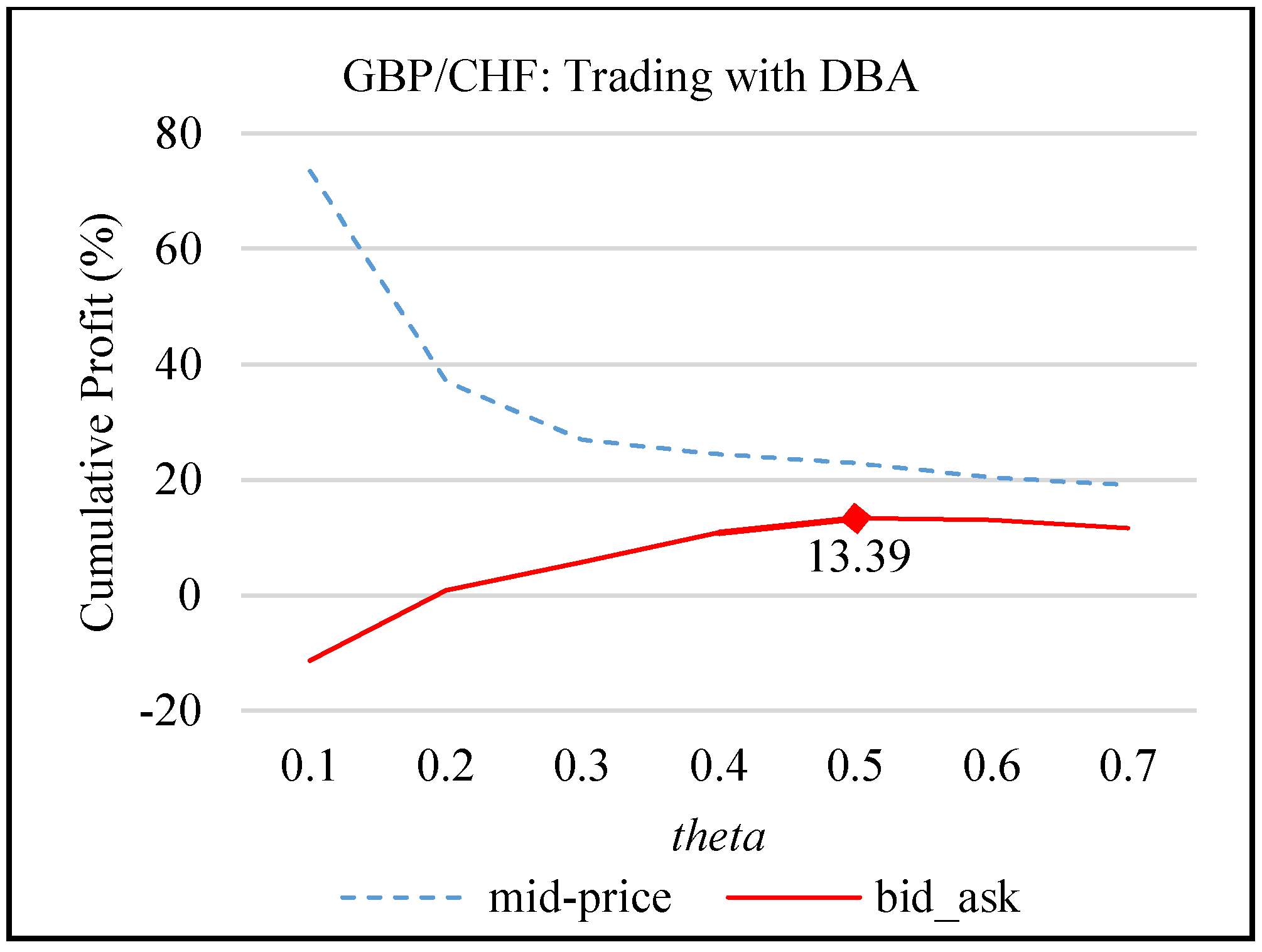
4.2. Finding the Value of down_ind
5. Intelligent Dynamic Backlash Agent: IDBA
5.1. The Learning Module
5.2. Calculating Order Size
5.2.1. The Independent Variables
5.2.2. C4.5
- All samples in the list belong to the same class. When this happens, it simply creates a leaf node for the decision tree saying to choose that class.
- None of the features provide any information gain. In this case, C4.5 creates a decision node higher up the tree using the expected value of the class.
- Instance of previously-unseen class encountered. Again, C4.5 creates a decision node higher up the tree using the expected value.
5.2.3. Computing the Order Size
- -
- denote the number of correctly classified instances of .
- -
- denotes the number of instances of falsely predicted to be .
- -
- denote the number of instance of falsely predicted to be .
- -
- denote the number of correctly classified instances of .
- if , then
- otherwise,
5.3. Risk Management
5.4. IDBA
- 1.
- During the training period:
- (a)
- It uses the trading parameters’ learning module described in Section 5.1 to determine the value of the trading parameters and down_ind. The learning module returns the best couple of trading parameters, namely and best_down_ind, corresponding to the highest returns.
- (b)
- IDBA employs the values and best_down_ind from point (a) to trade over the training period to compute the independent variables and and the dependent variable to train the forecasting model. It then employs the values of , , and to train the C4.5 algorithm. It computes the order size parameters and based on the performance of C4.5 as described in Section 5.2.
- (c)
- IDBA computes the risk management threshold corresponding to the best couple of the trading parameters and best_down_ind from point (a) above.
- 2.
- During the trading period:
- (a)
- IDBA uses the values of and best_down_ind to decide when to trigger a buy order as per Rule DBA.1 (Section 4.1).
- (b)
- IDBA uses the forecasting module and order size parameters and to decide the size of an order (Section 5.2.3).
- (c)
- IDBA uses the risk threshold to decide when it should stop trading and re-start the training process all over while trading over the trading period (Section 5.3).
6. Datasets and Methodology
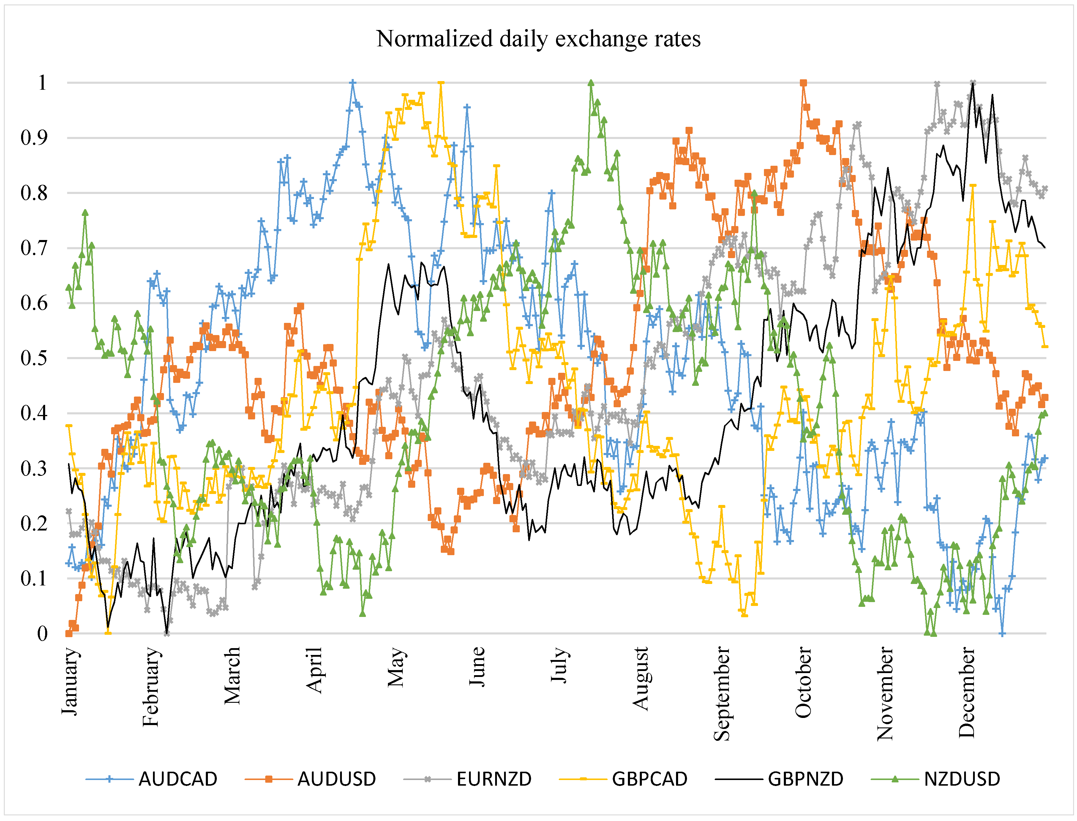
6.1. Data Selection
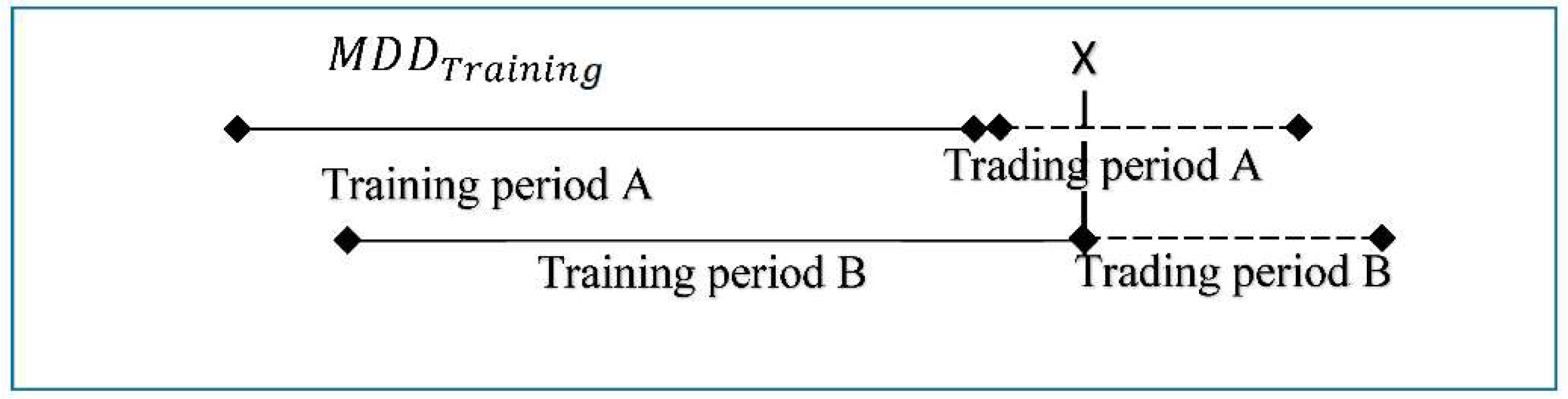
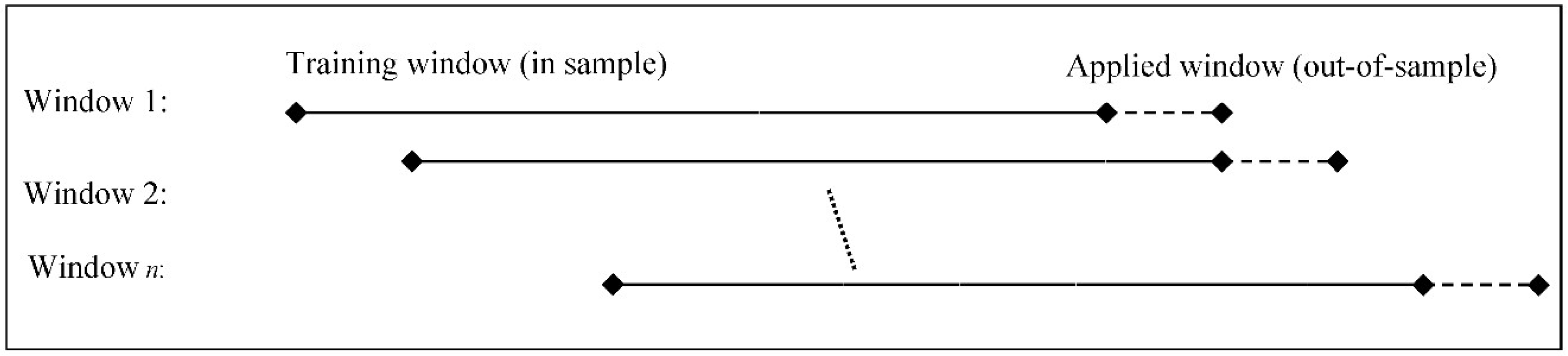
6.2. Preparing the Rolling Windows
7. Evaluation of IDBA: The Experiments
7.1. Experiment 1: Evaluating the Performance of IDBA
7.2. Experiment 2: Comparing IDBA with DBA
7.3. Experiment 3: Comparing IDBA with Another DC-Based Trading Strategy
8. Experiments: Results and Discussion
8.1. Experiment 1: Evaluating the Performance of IDBA
Experiment 1: Results’ Discussion
8.2. Experiment 2: Comparing IDBA with DBA
8.3. Experiment 3: Comparing IDBA with TSFDC
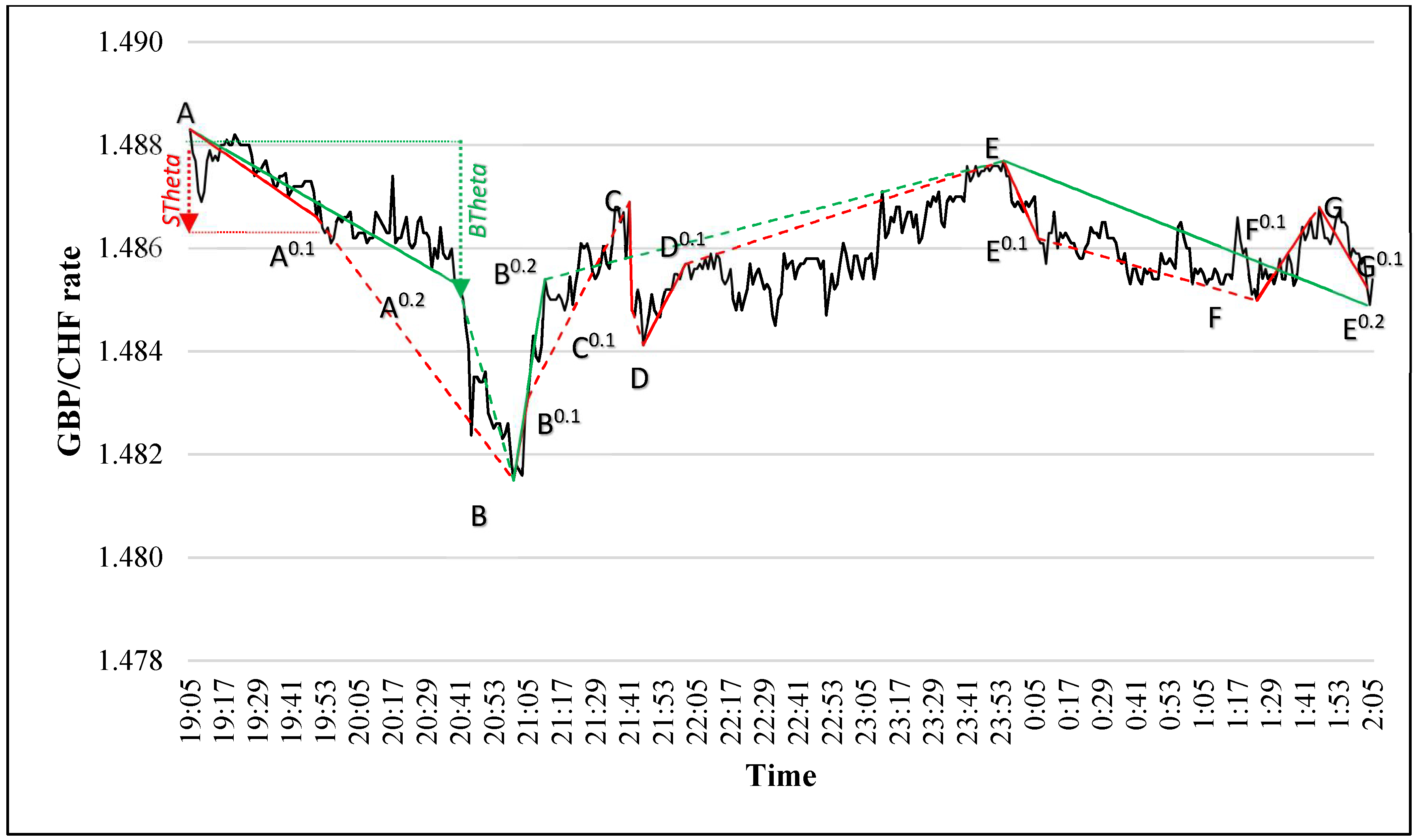
- TSFDC relies on the forecasting model developed by Bakhach et al. [6] to decide when to initiate a trade, whereas, IDBA uses a different forecasting model to control order’s size.
- TSFDC consists of tracking price changes using two DC thresholds, STheta and BTheta, whereas IDBA uses only one DC threshold.
- The traders must decide the values of the parameters STheta and BTheta, whereas IDBA has an embedded learning module to find the values of the trading partners and best_down_ind (Section 5.1).
- Both trading strategies open contrarian position.
- They both close these positions at the next DC confirmation point for the succeeding DC trend.
9. Conclusions
Author Contributions
Funding
Conflicts of Interest
References
- Guillaume, D.; Dacorogna, M.; Davé, R.; Müller, U.; Olsen, R.; Pictet, O. From the bird’s eye to the microscope: A survey of new stylized facts of the intra-daily foreign exchange markets. Financ. Stoch. 1997, 1, 95–129. [Google Scholar] [CrossRef]
- Ao, H.; Tsang, E. Capturing Market Movements with Directional; Working Paper WP069-13; Centre for Computational Finance & Economic Agents (CCFEA), University of Essex: Colchester, UK, 2013. [Google Scholar]
- Glattfelder, J.; Dupuis, A.; Olsen, R. Patterns in high-frequency FX data: Discovery of 12 empirical scaling laws. Quant. Financ. 2011, 11, 599–614. [Google Scholar] [CrossRef]
- Bisig, T.; Dupuis, A.; Impagliazzo, V.; Olsen, R. The scale of market quake. Quant. Financ. 2012, 12, 501–508. [Google Scholar] [CrossRef]
- Masry, S. Event-Based Microscopic Analysis of the FX Market. Ph.D. Thesis, Centre for Computational Finance & Economic Agents (CCFEA), University of Essex, Colchester, UK, 2013. [Google Scholar]
- Bakhach, A.; Tsang, E.P.; Jalalian, H. Forecasting Directional Changes in the FX Markets. In Proceedings of the IEEE Symposium on Computational Intelligence for Financial Engineer & Economic (CIFEr’ 2016), Athens, Greece, 6–9 December 2016. [Google Scholar]
- Alkhamees, N.; Fasli, M. Event detection from time-series streams using directional change and dynamic threshold. In Proceedings of the IEEE International Conference on Big Data (Big Data), Boston, MA, USA, 11–14 December 2017. [Google Scholar]
- Tsang, E.P.K.; Tao, R.; Serguieva, A.; Ma, S. Profiling Financial Market Dynamics under Directional Changes. Quant. Financ. 2017, 17, 217–225. [Google Scholar] [CrossRef]
- Tsang, E.; Chen, J. Regime change detection using directional change indicators in the foreign exchange market to chart Brexit. IEEE Trans. Emerg. Technol. Comput. Intell. 2018, 2, 185–193. [Google Scholar] [CrossRef]
- Aloud, M.E. Directional-Change Event Trading Strategy: Profit-Maximizing Learning Strategy. In Proceedings of the Seventh International Conference on Advanced Cognitive Technologies and Applications, Nice, France, 22 March 2015. [Google Scholar]
- Kampouridis, M.; Otero, F.E. Evolving trading strategies using directional changes. Expert Syst. Appl. 2017, 73, 145–160. [Google Scholar] [CrossRef]
- Golub, A.; Glattfelder, J.B.; Olsen, R.B. The Alpha Engine: Designing an Automated Trading Algorithm. In High-Performance Computing in Finance: Problems, Methods, and Solutions; Vynckier, E., Kanniainen, J., Keane, J., Dempster, M.A.H., Eds.; CRC Press: Boca Raton, FL, USA, 2017. [Google Scholar]
- Bakhach, A.; Tsang, E.P.; Chinthalapati, V.R. TSFDC: A trading strategy based on forecasting directional change. Intell. Syst. Account. Financ. Manag. 2018, 25, 105–123. [Google Scholar] [CrossRef]
- Bakhach, A.; Tsang, E.P.K.; Ng, W.L.; Chinthalapati, V.L.R. Backlash Agent: A trading strategy based on Directional Change. In Proceedings of the IEEE Symposium on Computational Intelligence for Financial Engineer & Economic (CIFEr’ 2016), Athens, Greece, 6–9 December 2016. [Google Scholar]
- De Faria, E.; Albuquerque, M.P.; Gonzalez, J.; Cavalcante, J.; Albuquerque, M.P. Predicting the Brazilian stock market through neural networks and adaptive exponential smoothing methods. Expert Syst. Appl. 2009, 36, 12506–12509. [Google Scholar] [CrossRef]
- Krollner, B.; Vanstone, B.; Finnie, G. Financial time series forecasting with machine learning techniques: A survey. In Proceedings of the European Symposium on Artificial Neural Networks: Computational and Machine Learning, Bruges, Belgium, 28–30 April 2010. [Google Scholar]
- Aldridge, I. High-Frequency Trading; Wiley Trading Series; John Wiley & Sons: Hoboken, NJ, USA, 2013. [Google Scholar]
- Vella, V.; Ng, W.L. A Dynamic Fuzzy Money Management Approach for Controlling the Intraday Risk-Adjusted Performance of AI Trading Algorithms. Intell. Syst. Acc. Financ. Manag. 2015, 22, 153–178. [Google Scholar] [CrossRef]
- Pardo, R. The Evalution and Optimization of Trading Strategy; John Wiley & Sons: Hoboken, NJ, USA, 2011. [Google Scholar]
- Sortino, F.; van der Meer, R. Downside risk. J. Portf. Manag. 1991, 17, 27–31. [Google Scholar] [CrossRef]
- Vanstone, B.J.; Hahn, T.; Finnie, G. Developing High-Frequency Foreign Exchange Trading Systems. In Proceedings of the 25th Australasian Finance and Banking Conference, Sydney, Australia, 16–18 December 2012. [Google Scholar]
- Sharpe, W.F. Asset allocation: Management Style and Performance Measurement. J. Portf. Manag. 1992, 18, 7–19. [Google Scholar] [CrossRef]
- Prokop, J. Further evidence on the role of ratio choice in hedge fund performance evaluation. J. Financ. Investig. Anal. 2012, 1, 181–195. [Google Scholar]
- Auer, B.R.; Schuhmacher, F. Robust evidence on the similarity of sharpe ratio and drawdown-based hedge fund performance rankings. J. Int. Financ. Mark. Inst. Money 2013, 24, 153–165. [Google Scholar] [CrossRef]
- Treynor, J.L. How to rate management of investment funds. Harv. Bus. Rev. 1965, 43, 63–75. [Google Scholar]
- Aloud, M.; Tsang, E.K.; Olsen, R. Modelling the FX market traders’ behaviour: An agent-based approach. In Simulation in Computational Finance and Economics: Tools and Emerging Applications; Alexandrova-Kabadjova, B., Martinez-Jaramillo, S., Garcia-Almanza, A., Tsang, E., Eds.; IGI Global: Hershey, PA, USA, 2012. [Google Scholar]
- Golub, A.; Chliamovitch, G.; Dupuis, A.; Chopard, B. Multiscale representation of high frequency market liquidity. Algorithm. Financ. 2016, 5, 3–19. [Google Scholar] [CrossRef]
- Quinlan, J. C4.5: Programs for Machine Learning; Morgan Kaufmann Publishers Inc.: San Francisco, CA, USA, 1993. [Google Scholar]
- Kearns, M.; Kulesza, A.; Nevmyvaka, Y. Empirical limitations on High-Frequency Trading Profitability. J. Trading 2010, 5, 50–62. [Google Scholar] [CrossRef]
- Evans, C.; Pappasa, K.; Xhafab, F. Utilizing artificial neural networks and genetic algorithms to build an algotrading model for intra-day foreign exchange speculation. Math. Comput. Model. 2013, 58, 1249–1266. [Google Scholar] [CrossRef]
- Bohn, S. The Slippage Paradox. 14 March 2011. Available online: http://arxiv.org/pdf/1103.2214 (accessed on 22 June 2017).
- Wilcoxon, F. Individual comparisons by ranking methods. Biom. Bull. 1945, 1, 80–83. [Google Scholar] [CrossRef]
- Vortelinos, D.; Koulakiotis, A.; Tsagkanos, A. Intraday analysis of macroeconomic news surprises and asymmetries in mini-futures markets. Res. Int. Bus. Financ. 2017, 39, 150–168. [Google Scholar] [CrossRef]
- Dupuis, A.; Olsen, R. High Frequency Finance: Using Scaling Laws to Build Trading Models. In Handbook of Exchange Rates; James, J., Marsh, I.W., Sarno, L., Eds.; John Wiley & Sons: Hoboken, NJ, USA, 2012; pp. 563–582. [Google Scholar]


| Time | Mid-Price | Point | |
|---|---|---|---|
| 20:55:00 | 1.48260 | 1.48260 | |
| 20:56:00 | 1.48230 | 1.48230 | |
| 20:57:00 | 1.48240 | 1.48230 | |
| 20:58:00 | 1.48260 | 1.48230 | |
| 20:59:00 | 1.48200 | 1.48200 | |
| 21:00:00 | 1.48150 | 1.48150 | B (Extreme point) |
| 21:01:00 | 1.48180 | 1.48150 | |
| 21:02:00 | 1.48170 | 1.48150 | |
| 21:03:00 | 1.48159 | 1.48150 | |
| 21:04:00 | 1.48280 | 1.48150 | |
| 21:05:00 | 1.48310 | 1.48150 | B0.1 (DCC point) |
| Time | Mid-Price | DC Event | Point | ||
|---|---|---|---|---|---|
| 21:41:00 | 1.48690 | start DC event (DOWNTREND) | C | ||
| 21:42:00 | 1.48480 | start OS event (DOWNTREND) | 1.48541310 | C0.1 | −0.41274713 |
| 21:43:00 | 1.48470 | −0.48006847 | |||
| 21:44:00 | 1.48520 | −0.14346177 | |||
| 21:45:00 | 1.48495 | −0.31176512 | |||
| 21:46:00 | 1.48412 | start DC event (UPTREND) | D | −0.87053224 | |
| ……………………… | |||||
| 22:01:00 | 1.48570 | start OS event (UPTREND) | 1.48560412 | D0.1 | 0.0645394 |
| Time | Mid-Price | DC Event | Point | ||
|---|---|---|---|---|---|
| 21:41:00 | 1.48690 | start DC event (DOWNTREND) | C | 2.64231213 | |
| 21:42:00 | 1.48480 | start OS event (DOWNTREND) | 1.48541310 | C0.1 | −0.41274713 |
| 21:43:00 | 1.48470 | −0.48006847 | |||
| 21:44:00 | 1.48520 | −0.14346177 |
| Actual | |||
|---|---|---|---|
| Predicted | |||
| Rolling Window | Training Period (12 Months) | Trading Period (1 Month) | ||
|---|---|---|---|---|
| From | To | From | To | |
| 1 | 1 January 2016 | 31 December 2016 | 1 January 2017 | 31 January 2017 |
| 2 | 1 February 2016 | 31 January 2017 | 1 February 2017 | 28 February 2017 |
| 3 | 1 March 2016 | 28 February 2017 | 1 March 2017 | 31 March 2017 |
| 4 | 1 April 2016 | 31 March 2017 | 1 April 2017 | 30 April 2017 |
| 5 | 1 May 2016 | 30 April 2017 | 1 May 2017 | 31 May 2017 |
| 6 | 1 June 2016 | 31 May 2017 | 1 June 2017 | 30 June 2017 |
| 7 | 1 July 2016 | 30 June 2017 | 1 July 2017 | 31 July 2017 |
| 8 | 1 August 2016 | 31 July 2017 | 1 August 2017 | 31 August 2017 |
| 9 | 1 September 2016 | 31 August 2017 | 1 September 2017 | 30 September 2017 |
| 10 | 1 October 2016 | 30 September 2017 | 1 October 2017 | 31 October 2017 |
| 11 | 1 November 2016 | 31 October 2017 | 1 November 2017 | 30 November 2017 |
| 12 | 1 December 2016 | 30 November 2017 | 1 December 2017 | 31 December 2017 |
| Mean | Standard Deviation | Quantile 25 | Quantile 75 | |
|---|---|---|---|---|
| AUD/USD | 0.000061 | 0.000051 | 0.000050 | 0.000060 |
| AUD/CAD | 0.000010 | 0.000090 | 0.000120 | 0.000150 |
| GBP/CAD | 0.000266 | 0.000237 | 0.000190 | 0.000240 |
| GBP/NZD | 0.000508 | 0.000325 | 0.000390 | 0.000480 |
| NZD/USD | 0.000093 | 0.000071 | 0.000010 | 0.000090 |
| EUR/NZD | 0.000347 | 0.000245 | 0.000260 | 0.000320 |
| Currency Pair | RR | Profit Factor | Total Number of Trades | Max Drawdown (%) | Win Ratio | Sharpe Ratio |
|---|---|---|---|---|---|---|
| AUD/USD | 23.5 | 1.86 | 1143 | 1.5 | 0.77 | 2.89 |
| AUD/CAD | 26.2 | 1.92 | 1182 | 1.7 | 0.76 | 4.55 |
| GBP/CAD | 4.3 | 1.09 | 986 | 2.6 | 0.64 | 0.83 |
| GBP/NZD | 29.8 | 2.35 | 1892 | 1.7 | 0.78 | 4.62 |
| NZD/USD | 18.8 | 1.42 | 1068 | 3.4 | 0.75 | 1.59 |
| EUR/NZD | 16.1 | 1.87 | 1079 | 2.2 | 0.73 | 1.29 |
| Trading Period | AUD/USD | AUD/CAD | GBP/CAD | GBP/NZD | NZD/USD | EUR/NZD |
|---|---|---|---|---|---|---|
| January | 1.4 | 2.0 | 0.7 | 2.0 | 1.9 | 1.2 |
| February | 2.5 | 2.4 | 0.6 | 2.1 | 2.2 | 1.5 |
| March | 0.5 | 2.7 | −0.3 | 2.3 | 1.1 | 2.2 |
| April | 2.4 | 2.5 | −0.2 | 2.4 | 0.1 | 3.2 |
| May | 2.1 | 1.9 | 0.9 | 1.7 | 1.9 | 1.5 |
| June | 1.9 | 2.3 | 0.5 | 2.5 | 2.2 | 2.4 |
| July | 3.0 | 2.4 | 0.6 | 3.6 | 2.5 | 0.4 |
| August | 1.1 | 3.0 | −0.1 | 2.2 | 1.9 | 1.1 |
| September | 2.7 | 2.3 | −0.3 | 2.5 | 1.6 | 1.2 |
| October | 1.8 | 1.1 | 0.7 | 3.4 | 0.8 | 2.0 |
| November | 1.8 | 1.9 | 0.5 | 2.9 | 1.9 | 0.6 |
| December | 2.3 | 1.7 | 0.7 | 2.2 | 2.5 | 0.8 |
| Sum | 23.5 | 26.2 | 4.3 | 29.8 | 18.8 | 16.1 |
| AUD/USD | AUD/CAD | GBP/CAD | GBP/NZD | NZD/USD | EUR/NZD |
|---|---|---|---|---|---|
| 6 | 5 | 7 | 6 | 5 | 5 |
| Currency Pairs | RR | MDD | ||
|---|---|---|---|---|
| IDBA | DBA | IDBA | DBA | |
| AUD/USD | 23.5 | 11.2 | 1.5 | 6.7 |
| AUD/CAD | 26.2 | 10.7 | 1.7 | 4.9 |
| GBP/CAD | 4.3 | 3.4 | 2.6 | 5.8 |
| GBP/NZD | 29.8 | 15.5 | 1.7 | 6.5 |
| NZD/USD | 18.8 | −0.7 | 3.4 | 6.2 |
| EUR/NZD | 16.1 | 6.9 | 2.2 | 7.5 |
| RR | MDD | |
|---|---|---|
| p-value | 0.026 | 0.005 |
| Currency Pairs | RR | MDD | ||
|---|---|---|---|---|
| IDBA | TSFDC | IDBA | TSFDC | |
| AUD/USD | 23.5 | 24.2 | 1.5 | 7.8 |
| AUD/CAD | 26.2 | 24.1 | 1.7 | 8.6 |
| GBP/CAD | 4.3 | 5.6 | 2.6 | 12.2 |
| GBP/NZD | 29.8 | 30.5 | 1.7 | 4.6 |
| NZD/USD | 18.8 | 19.7 | 3.4 | 7.4 |
| EUR/NZD | 16.1 | 17.2 | 2.2 | 10.5 |
| RR | MDD | |
|---|---|---|
| p-value | 0.937 | 0.002 |
© 2018 by the authors. Licensee MDPI, Basel, Switzerland. This article is an open access article distributed under the terms and conditions of the Creative Commons Attribution (CC BY) license (http://creativecommons.org/licenses/by/4.0/).
Share and Cite
Bakhach, A.; Chinthalapati, V.L.R.; Tsang, E.P.K.; El Sayed, A.R. Intelligent Dynamic Backlash Agent: A Trading Strategy Based on the Directional Change Framework. Algorithms 2018, 11, 171. https://doi.org/10.3390/a11110171
Bakhach A, Chinthalapati VLR, Tsang EPK, El Sayed AR. Intelligent Dynamic Backlash Agent: A Trading Strategy Based on the Directional Change Framework. Algorithms. 2018; 11(11):171. https://doi.org/10.3390/a11110171
Chicago/Turabian StyleBakhach, Amer, Venkata L. Raju Chinthalapati, Edward P. K. Tsang, and Abdul Rahman El Sayed. 2018. "Intelligent Dynamic Backlash Agent: A Trading Strategy Based on the Directional Change Framework" Algorithms 11, no. 11: 171. https://doi.org/10.3390/a11110171
APA StyleBakhach, A., Chinthalapati, V. L. R., Tsang, E. P. K., & El Sayed, A. R. (2018). Intelligent Dynamic Backlash Agent: A Trading Strategy Based on the Directional Change Framework. Algorithms, 11(11), 171. https://doi.org/10.3390/a11110171