Article

2-Phase NSGA II: An Optimized Reward and Risk Measurements Algorithm in Portfolio Optimization

by
Seyedeh Elham Eftekharian
1,*,
Mohammad Shojafar
2 and
Shahaboddin Shamshirband
3,4,*
1
Department of Financial Engineering, Raja University of Qazvin, Qazvin 341451177, Iran
2
Department of Information Engineering, Electronics and Telecommunications, University of Rome Sapienza, Via Eudossiana 18, 00184 Rome, Italy
3
Department for Management of Science and Technology Development, Ton Duc Thang University, Ho Chi Minh City, Vietnam
4
Faculty of Information Technology, Ton Duc Thang University, Ho Chi Minh City, Vietnam
*
Authors to whom correspondence should be addressed.
Algorithms 2017, 10(4), 130; https://doi.org/10.3390/a10040130
Submission received: 17 October 2017 / Revised: 17 November 2017 / Accepted: 23 November 2017 / Published: 28 November 2017
(This article belongs to the Special Issue Evolutionary Computation for Multiobjective Optimization)

Abstract

:
Portfolio optimization is a serious challenge for financial engineering and has pulled down special attention among investors. It has two objectives: to maximize the reward that is calculated by expected return and to minimize the risk. Variance has been considered as a risk measure. There are many constraints in the world that ultimately lead to a non–convex search space such as cardinality constraint. In conclusion, parametric quadratic programming could not be applied and it seems essential to apply multi-objective evolutionary algorithm (MOEA). In this paper, a new efficient multi-objective portfolio optimization algorithm called 2-phase NSGA II algorithm is developed and the results of this algorithm are compared with the NSGA II algorithm. It was found that 2-phase NSGA II significantly outperformed NSGA II algorithm.

Graphical Abstract

1. Introduction

Portfolio optimization is a bi-objective optimization problem aimed at maximizing the reward and at the same time, minimizing the risk. The reward and the risk of portfolio are estimated by the mean of return and the variance of return, respectively [1,2].
It is unlikely to come across an optimal solution in a multi-objective optimization problem since the employed objective functions often conflict with each other and it is impossible to optimize all objective functions at the same time. Instead, a set of best solutions which came to be known as efficient frontier is obtained and authorized many alternatives to decision maker who choose the solution that is most suited to a particular application. Apart from the constraint of ensuring that all money has been invested (budget constraint), there are some other constraints in the real-world [3]. One of these constraints is cardinality constraint that limits the number of assets in portfolio [4]. This constraint leads to introducing integer variables. Therefore, the results of a mixed integer optimization problem are multiple local exterma and discontinuities [5,6,7]. Indeed, authors in [7] present GAMCC as a genetic-aware credit crunch constraint applied in an intelligent model in bank lending decisions. It maximizes the bank profit and minimizes the probability of bank default in a search for a dynamic lending decision. The big limitation of the method compared our model is time and global optimization which is covered in the proposed method and has been confirmed in the simulation. Because of a complex problem as a result of additional constraints, classical optimization methods do not work and so, heuristic optimization techniques need to be applied in order to find optimal or near optimal solutions. Authors in [8] exemplifies one of the first uses of heuristics to portfolio selection. They applied semi-variance as a risk measure and utilized threshold accepting in a portfolio selection problem. The big gap they did not address the risk constrained raised in portfolio selection problem. So their threshold needs to be tuned to be applied in scale case which is covered in our solution. Also, the reference [3] introduced cardinality constraint and quantity constraint for portfolio selection problem and solved the new model by three heuristic algorithms, i.e., genetic algorithms, tabu search and simulated annealing. Authors in [9,10] studied the capability of heuristic techniques, namely NSGA II, PESA and SPEA, for overcoming complex portfolio optimization problem. They replaced variance as an index of risk with value at risk and expected shortfall. The aforementioned solution did not address the mutual portfolio risk effect in the portfolio selection problem that is accounted in the proposed method. A new objective function related to the number of securities in the portfolio was added to two former objectives of risk and return of the portfolio by [11]. Moreover, quantity and class limitations are imposed to the model and they solved it by three evolutionary multi-objective algorithms, namely NSGA II, PESA and SPEA2. On the other hand, authors in [12] suggested an order–based representation for the integration of realistic constraints with the portfolio optimization problem model [13] and included preference criterion in the optimization search process and addressed evolutionary multi-objective portfolio optimization for both of them. In [14] authors presented two intelligent trading systems in which exploits fuzzy logic techniques to enhance the power of genetic procedures and attempts to improve the performances of fuzzy system through Neural Networks. Although the method is interesting, compared with the proposed solution, it suffers from some realistic constraints. Later on, the same authors in [15] design a joint fuzzy-GSA system to tune suitable parameters of GSA, by impacting on the exploration, the exploitation capabilities and get ride of local optima using the fuzzy-manner choice of adjusting, that use fuzzy input and output altogether. The method is very neat and novel but it again did not cover some global effect limitations which are addressed in the proposed joint method. Besides, [16] proposed a new particle swarm optimization (PSO) to solve the Cardinality Constrained Markowitz Portfolio Optimization problem (CCMPO problem). This study proposes a new evolutionary algorithm, called 2-phase NSGA II, which is used for portfolio optimization problem. This algorithm is contrasted with non-dominated sorting genetic algorithm II (NSGA II). Our purpose is to survey if 2-phase NSGA II developed algorithm could outperform NSGA II efficiently.
The rest of the paper is classified as shown below. Section 2 reviews the literature. Section 3 describes the problem. Thereafter, in Section 4 we introduce 2-phase NSGA II and NSGA II algorithms. Section 5 is allocated to numerical results and compares the results of both algorithms. Finally, in Section 6 we outline the conclusions of this paper.

2. Related Work

Portfolio optimization has been used in several works with multiple objectives, and many heuristic algorithms have been applied for solving this problem. For example, authors in [17] proposed a decision making model for portfolio selection aimed at minimizing transaction lots. They solved the model with genetic algorithm (GA). Their method found the solution in a short reasonable time, but the current case that is the market is the only uncertainty in reality and some other risk cases must be added. Moreover, authors in [4] used simulated annealing (SA) for solving portfolio selection problem. The objective function of their model was to reduce portfolio risk, and expected return of investor was assigned and set as a constraint. The method is an efficient solution in the scope, however, it is still a complicated solution to manage due to the space of feasible portfolios that is simplified in our algorithm. A heuristic model based on neural network was developed by [18] and was handled for tracing efficiency curve. They compared their results with tabu search (TS), simulated annealing (SA), and genetic algorithm (GA). The presented model is indeed a combination of quadratic programming model and integer programming which none of exact algorithms could not solve this problem efficiently and consequently, the necessity of utilization of evolutionary algorithms (EAs) seems worthwhile for solving the problem. Moreover, authors in [19] solved portfolio optimization problem in terms of various risk criteria containing semi-variance, variance with skewness, and genetic algorithm. On the other hand, authors in [20] utilized a new neural network algorithm for selecting optimized portfolio based on investor preferences. The given model was based on mean, return, and skewness. They showed that the presented model led to the result in shorter time as compared to other models. The big drawback of the method is its inefficacy when face with the dynamic and uncertain environment and the risk can be tuned fairly. The paper [21] investigated particle swarm optimization (PSO) for solving portfolio selection problem. This method instead of finding the global optimal solution converges to a close optimal solution and won’t be a useful option for the uncertain dynamic risk-aware systems. Even though, [22] suggested an improved particle swarm optimization algorithm for the problem of selecting optimized portfolio with the assumption that there was some admissible error for both risk and return. Although this method resolves several raised limitations for the previous solutions it still faces problem in scalable uncertain markets. Authors in [23] considered a new factor called market capitalization in addition to transaction cost and the number of stocks in the portfolio constraints. They used genetic algorithm for solving the proposed model. This method seems could be salient and an efficient method applied in portfolio problem but we would that it has had some limitations for the various markets with hard boundaries and still has a problem in scalable uncertain markets. Besides, authors in [5] exploit threshold policy to control portfolio optimization and applied VaR, ES, mean absolute semi deviation and semi variance for risk measurements. In addition, [24] used quadratic programming for portfolio selection. Besides, the paper [25] applied greedy search, simulated annealing and ant colony optimization for portfolio problem. On the other hand, [26] used NSGA II, PESA and SPEA 2 for solving mean-variance portfolio optimization problem and [27] integrated evolutionary computations and linear programming to suggest a hybrid multi-objective optimization approach. Moreover, authors in [12] used multi-objective evolutionary algorithm presentation on an ordered basis. Reference [28] suggested a hybrid algorithm that integrated critical line algorithm and NSGA II. Furthermore, NSGA II, PESA and SPEA 2 in portfolio optimization problem was compared by [27]. Reference [11] considered third objective function of the number of securities in the portfolio except two other common objectives of risk and return. They obtained the optimized portfolio with using three evolutionary algorithms—namely NSGA II, PESA, and SPEA 2—and compared the results of these methods with each other. Standard portfolio selection problem has allocated excess volume of the researches and insignificant number of researches are related to portfolio selection in multi-objective case that has recently received great attention. Markowitz’s mean-variance portfolio optimization model proposed a learning-guided solution generation strategy considering four real-world constraints (cardinality, quantity, pre-assignment and round lot) and the results of the proposed algorithm were compared with four existing multi-objective Evolutionary Algorithms including NSGA-II, SPEA-2, PESA-II, and PAES by [29]. Moreover, [30] is the most popular research related to affrication of multi-criteria decision making (MCDM) in financial decision makings. Although this method belongs to the prevalent method in portfolio analysis research, it neither covers portfolio ranking nor decision support systems. Authors in [31] proposed an approach for portfolio production and selection related to return, variance skewness factors. Indeed, it was a development of Markowitz classic model and normal distribution assumption for returns was not necessary to be considered. Objective function of their model was to maximize the expected return and skewness of portfolio return and to minimize the risk simultaneously. However, given the fact that electricity market prices are not normally distributed but skewed, asset allocation based on the raised framework is more suitable than the Markowitz mean-variance ones so it is not a suitable solution in the risky environments. Another objective function except risk and return called “Entropy” was added to the multi-objective model [32]. They used fuzzy programming technique in order to solve the model which cause some inconsistency and local solution, especially with the complex case problems. Reference [33] mentioned that investors followed antithetic objectives in portfolio selection concurrently and proposed adaptive programming model with random constraint to combine adaptive programming model and programming model with random constraint. Moreover, authors in [34] introduced liquidity of assets as the most important factor of considering criteria of investors in the frame of standard portfolio optimization. Reference [9] investigated a multi-period portfolio optimization model in the market having both risky and risk-free securities. Although they used dynamic programming for their problem, compared with the proposed method, it fails to be validated with various generations and has more converging time. Recently, [35] utilized goal programming and multi-purpose genetic algorithm methods in Markowitz mean-variance model. The main limitation of such method is that it did not bound the constrained we addressed the same problem.

3. Statement of Problem and Notation

Because some real life situations are not considered in Markowitz model except the main assumption that returns are normally distributed, novel research directions are needed for portfolio models. One method is considering some constraints that have to be taken into account; e.g., restriction of the number of assets in the portfolio, limitation of investing in assets with common characteristics (investing in vehicle manufacturing industry, petrochemical industry, bank assets, etc.) and avoidance of very small holdings which are cardinality, class and quantity constraints, respectively. Admittedly, these constraints need discrete variables to be used to transfer the search space into a non-convex set. The present paper considers the following model:
min F 1 = i = 1 n j = 1 n x i x j σ i j max F 2 = i = 1 n x i μ i ,
subject to:
i = 1 n x i = 1 ,
l i δ i x i u i δ i ,
L m i C m n U m , m = 1 M ,
L m j C m n μ i U m , m = 1 M ,
σ { 0 , 1 } , i = 1 n ,
where, n is the number of available assets, k is the number of assets in the portfolio, σ i j shows the covariance between assets i and j, μ i determines the mean return of the portfolio, and x = ( x 1 , , x n ) represents the proportion weights of initial budget that is allocated to each asset. Equation (2) is budget constraint that insures all available capital is invested. Equations (3) and (4) are cardinality and quantity constraints, respectively, both of which have binary variable of δ i . If asset i holds in the portfolio δ i = 1 else δ i = 0 . The former shows that k assets exist in the portfolio and the latter considers lower and upper bounds for each existent asset in the portfolio. Equation (5) shows class constraint and for all ij, C i C j = that means there are unique sets of assets. Two points should be considered in this constraint:
(i)
L m > 0 for m = 1 , , M , This limitation ensures that at least one asset from each class should be chosen;
(ii)
k M , which means the portfolio should have more assets that classes (this note is concluded from the first point).
Also, F 1 and F 2 are the risk and return of the optimal portfolios, respectively. Since there are two contradictory objectives, it is not possible to obtain single optimal solution; rather, a set of solutions called Pareto-optimal solutions is found and contains all feasible solutions not dominated by any other solution in the feasible set. It is said that solution x 1 dominates solution x 2 if:
F 2 ( x 1 ) > F 2 ( x 2 ) a n d F 1 ( x 1 ) F 1 ( x 2 )
or
F 2 ( x 1 ) F 2 ( x 2 ) a n d F 1 ( x 1 ) < F 1 ( x 2 )

4. Methodologies

4.1. NSGA II Algorithm

It is a kind of genetic algorithm which operates according to dominance and non-dominance relation to determine Pareto solutions. A population of size N is considered and the solutions are sorted according to non-dominated sorting, by which it could be distinguished at which frontier a solution is situated. The non-dominated solutions are located in the first front and are given rank 1. Then, the solutions are eliminated and the second frontier of non-dominated solutions is recognized given rank 2. The process goes on until all solutions in the population are categorized. The solutions with the same rank were selected by crowding distance mechanism that works as follows. After sorting the individuals in the last cited front according to each objective function in an increasing order, the amount of infinite distance value is assigned to both solutions with the largest and smallest objective function values (boundary solutions) so that they are always selected. The overall crowding distance value is computed as total distance of each objective function. The crowding distance of remaining solutions is the mean side length of the cuboids formed by using the two adjacent solutions as the vertices. If the crowding distance of a solution is smaller, it implies that it is crowded by other solutions [36].

4.2. The Proposed 2-Phase NSGA II Algorithm

This algorithm has been proposed for two reasons. First, it avoids the gaps in the Pareto-optimal front and second, it helps the improvement of Pareto-optimal solutions. The former makes a better diversification and discovers a well-distributed set of non-dominated solutions along with Pareto-optimal front. The latter lets us to investigate if it is feasible to improve the Pareto-optimal solutions; thereby, the final solutions could be approximated to optimal front.
This algorithm has been divided into two phases. In the first phase, the groundwork is like the procedure of NSGA II. The Pareto-optimal solution derived from NSGA II is the input to the second phase.
In the new phase and with integrating all the obtained solutions from the first phase in a global archive and with using elitism strategy, we improve the quality of initial Pareto solutions that elicit from the first phase. Also, with running the second phase, it is expected not only solutions diversification is preserved but also the quality of them is improved. After deriving all Pareto solutions from the previous phase, we have to do two runs for finishing the algorithm. In the first run, we sort the solutions in a descending order. Then, the following model is followed for each consecutive solution in objective functions space:
Pr1:
min F 1 s t : F 1 f 1 1 F 2 f 2 2 F 2 f 2 1
where, f 1 1 and f 1 2 denote first objective function values for solutions 1 and 2, respectively and f 2 1 and f 2 2 determine second objective function values for the solutions 1 and 2, respectively. Each solution that is applicable to problem Pr1 could be placed in box S 1 or S 2 . If it is placed in box S 1 , node k locates on optimal front too; otherwise, there is a new solution improving last position and optimal front layer (Figure 1). This procedure is continued till all peer nodes are examined. It needs to be noted that we may not find a practical solution for pair nodes in stopping condition. In this situation, the algorithm is kept fixed for the first solution of pair nodes and is switched to the node which is next to pair. Finally, Pareto-optimal front is updated and the out coming real Pareto optimal set is archived.
In the second run as a supplementary step, after testing all nodes in the first run, F 2 and F 1 are placed in both objective and constraints and the procedure of improving and covering solutions in problem Pr1 is so that the improvement is possible in direction of first objective function. All above procedure for problem Pr1 is repeated for this model. Thus, problem Pr2 can be written as follows:
Pr2:
min F 2 s t : F 2 f 2 1 F 1 f 1 1 F 1 f 1 2
The possibility of improving and covering in direction of second objective function (Return) is possible by running this part. Figure 2 shows the improvement of Pareto-front by these two runs.
This method is very interesting since the gaps between the incoherent pieces of Pareto-front are filled by Pareto-optimal solutions.

4.3. The Algorithms Procedure

A random population P 0 should be created. Fitness function is calculated for each solution in P 0 according to Equation (8):
N R e t ( i ) = μ i i = 1 n μ i , i = 1 , , n ,
N R i s k ( i ) = 1 / p i i = 1 n 1 / p i , i = 1 , , n ,
F i t n e s s ( i ) = α × N R e t ( i ) + ( 1 α ) × N R i s k ( i ) , i = 1 , , n ,
where α is a random variable between 0 and 1 and maximization of fitness is desirable.
Three operators of selection, crossover and mutation are utilized to generate an offspring solution Q 0 (size N). Next, for all 2 N solutions of P 0 and Q 0 , non-dominated sorting is used and they were classified to some fronts. For creating the next generation, F 1 is transferred to the next generation thereafter, F 2 , and this process continues till the number of solutions exceeds N. At this stage, crowding distance value is used for the latest front and the solutions with larger distance are moved to P 1 till the size of P 1 becomes N. At last, this procedure is resumed for the next generations [36]. It should be noted that the study applies uniform selection for selecting parents. The details of the procedure are explained below:
(1)
Set t = 0 and produce the random population P 0 of size N.
(2)
Assess the objective functions and sort the solutions based on dominance and non-dominance relation operator.
(3)
Select the solutions as parents based on uniform selection.
(4)
Affect the selected solutions by crossover and mutation operators to produce offspring population Q 0 of size N.
(5)
Evaluate the new offspring based on objective functions.
(6)
R t = P 0 Φ 0 and sort the R t solution based on dominance and non-dominance relation (swift non-dominated kind) and make fronts ( F 1 , F 2 , ).
(7)
P t + 1 = and i = 1 .
(8)
Until | P t + 1 | + | F i | N , P t + 1 = P t + 1 F i , i = i + 1 .
(9)
If | P t + 1 | + | F i | N , calculate crowding distance for all solutions in F i .
(10)
Sort ( F i , < n )
(11)
P t + 1 = P t + 1 F i [ 1 : ( N | P t + 1 | ) ]
(12)
Stopping criteria: End the algorithm if the stopping criterion is met; otherwise, go to step 2.
We utilized representation scheme suggested by [37]. Three arrays of A, B and τ are used for representing the solutions. Array A consists of M cells filled randomly in [0, 1] and shows the weight of each class. These weights are obtained by Equation (11). Array B presents the existence of assets in the portfolio. The size of this array is equal to K and it is filled by integer numbers randomly. In order to satisfy the provision that at least one asset is selected from each class, we fill out the first M cells of array B by selecting one asset from each one of M classes. If K > M , the remaining K M are selected from the other assets which had not been chosen in the previous step. With respect to this array, cardinality constraint is satisfied since it has exactly a defined size in the model. Array τ prescribes the weight of each asset which attends in array B and has the size of N. The cells of assets that are not present in array B get zero weight. For example, if the fifth asset is not chosen, the fifth cell of array τ takes zero weight. The weights of assets which exist in the array B are calculated by Equation (14) and this weight is assigned to the opposing cells of array τ . The weight assigned to each class is calculated by:
C m = L m + r ( U m L m ) , m = 1 , , M ,
where, r is a random value between 0 and 1; C m is the amount of investing in class m; and L m and U m are the lower and the upper bound for class m, respectively. By this equation we ensure that all the weights are within their bounds. To be sure that the sum of the weights equals 1, we use the following equation (standard normalize):
C ^ m = C m m = 1 M C m , m = 1 , , M ,
where C ^ m is the normalized C m .
Moreover, the weight invested in each asset is calculated by the following formula:
w i = l i δ i + r ( u i δ i l i δ i ) , i = 1 , , N ,
where, w i is the random weight of asset i and it is within its lower and upper bound. Therefore, this equation satisfies considering the lower and upper limits for assets, which is called quantity constraint. For satisfaction of the sum to one constraint Equation (14) is used:
x i = w i δ i i c l a s s ( i ) N w i δ i × C c l a s s ( i ) , i = 1 , , N ,
where, x i is the actual amount that will be invested in each asset and c l a s s ( i ) shows the class of each selected asset that is an array with K cells and we call it ”class array”. The first M cells take values 1 to M because the first M cells of array B are filled by selecting one asset from each class and the remaining K M cells take the values associated to K M cells of the array B. For instance, if cell M + 1 of array B contains an asset which belongs to class 6, the value 6 is placed in the cell M + 1 of class array, and, so on.
By this encoding method, feasible solutions will be often found. However, in some cases it is possible to find an infeasible solution and thus the solution should be repaired. Three repairing mechanisms are explained here:
(1)
After normalizing array A, the weight of one or more classes may not be within the lower and upper limits. For overbearing this problem, the weight of that class or those classes should be calculated again using Equation (11). This process is continued until the weight of all classes lies within their lower and upper limits.
(2)
The weight of each class should equal the sum of the weights of the assets existed in that class. When there is only one asset in a given class, it is clear that the weight of this asset is unlikely to be equal to the weight of the class that it belongs to. Therefore, we consider the weight of the class for the asset and investigate whether this new weight satisfies quantity constraint. If this provision is not confirmed, the weight is calculated for the second time. If the weight violates the upper limit, the new weight is replaced with upper limit and the other weights are normalized again. This process continues until all weights are located in the lower and upper bounds span.
(3)
Given the fact that selecting at least one asset from each class is essential in the model ( L m > 0 ), we are assured of choosing one asset from each class at the same time as filling the cells of B chromosome.

4.4. Genetic Operators

In order to generate the offspring population, the uniform crossover and the following mutation operators are utilized.
C i m u t = p ( c i L i ) L i , i = 1 , , M ,
w j m u t = p ( w j l j ) l j , j = 1 , , K ,
where, p is the step value and is selected randomly between 0 and 1. The crossover operator is used for arrays B and τ simultaneously. It means if assets of the same cells of two parents’ chromosome are transferred, their weights in array τ should be dislocated. For doing mutation in array B, a value from M + 1 to K is selected randomly and the asset existing in this cell is substituted with another asset from the whole set so that there is at least a ”representative” from each class in the portfolio. The weight of this new selected asset should be inevitably attained by Equation (13) and the entire repair mechanisms have to be done till all the solutions satisfy the considered constraints.

5. Performance Evaluation

A vast computational study is carried out for the evaluation of the effectiveness of the new algorithm and its comparison with NSGA II algorithm. The comparison between NSGA II and 2-phase NSGA II algorithms is done according to the sets of non-dominated solutions obtained by both algorithms.

5.1. Scenario Description

In this subsection we aim to present the scenario we test our solutions on it.

5.1.1. Data Sets

Five test problems based on the stocks involved in five various capital market indices derived from around the world were applied for the testing of algorithms. They included the hang seng (Hong Kong), Dax 100 (Germany), FTSE 100 (UK), S&P 100 (US) and Nikkei 225 (Japan). These data were supplied by Beasley (http://people.brunel.ac.uk/umastjjb/jeb/orlib/portinfo.html). The returns and covariances were calculated by 291 values and the size of these five test problems varied in the range of N = 31 (Hang Seng) to N = 225 (Nikkei). The details of these groups of assets are summarized in Table 1.

5.1.2. Comparison Metrics

In most multi-objective optimization methodologies, the Pareto-optimal front is approximated by a set of non-dominated solutions. We should note that the quality of these solutions depends on how they are evaluated, since there are some contractions and inconsistencies in the nature of some of the criteria complicating this process. Admittedly, it is not straight to compare the solutions of two distinct Pareto-sets obtained from solving two algorithms. In the 1990s, the visual inspection was applied to evaluate the quality of solutions to the Pareto-optimal front in the objective space. Nevertheless, the quality of the obtained Pareto-sets must be estimated by a quantitative metric. Therefore, we introduced five indices as following in the present work:
(1)
MID (mean ideal distance): the sum of distances between Pareto solutions and ideal point [38];
(2)
NPS: number of solutions in the Pareto-front;
(3)
MS: the maximum spread that is the Euclidean distance between boundary solutions;
(4)
S: the spacing which is proceeded to calculate the space between two adjacent solutions;
(5)
CS: the coverage set which is used to survey the preference of the algorithms.
The formulas used to calculate these metrics are given in Table 2.

5.1.3. Parameter Settings

The competency of the algorithms depends on selecting the best parameters. The parameters that influence the performance of the algorithms applied in this study are the number of generation ( N o G ), crossover and mutation rates ( C R , M R ), k, M and population size ( p o p s i z e ). Before executing the algorithm, it was adjusted to detect fine parameter values that allow them run well, according to which crossover and mutation probability were set at 0.8 and 0.2, respectively. Additionally, the distinguished parameters applied for each problem are presented in Table 3. Stopping criteria for NSGA II algorithm is the number of generation but this criterion for 2-phase NSGA II is different. Regarding the exponential accession of the number of Pareto solutions, considering many iteration of generations is illogical and expenditure. In order to eliminate this problem, we performed each problem for twenty times and concluded that the number of Pareto solutions is considered to be stopping criteria. Based on the results, each test problem (port 1 to port 5) is stopped after finding 4500, 8000, 8000, 10,000 and 15,000 solutions in Pareto archive, respectively.

5.2. Experimental Results

This sub-section compares the proposed 2-phase NSGA II with the known NSGA II algorithm. Both algorithms were implemented in MATLAB on a laptop Core 2 Duo at 2 GHz with 4 GB RAM under Windows Vista operating system.
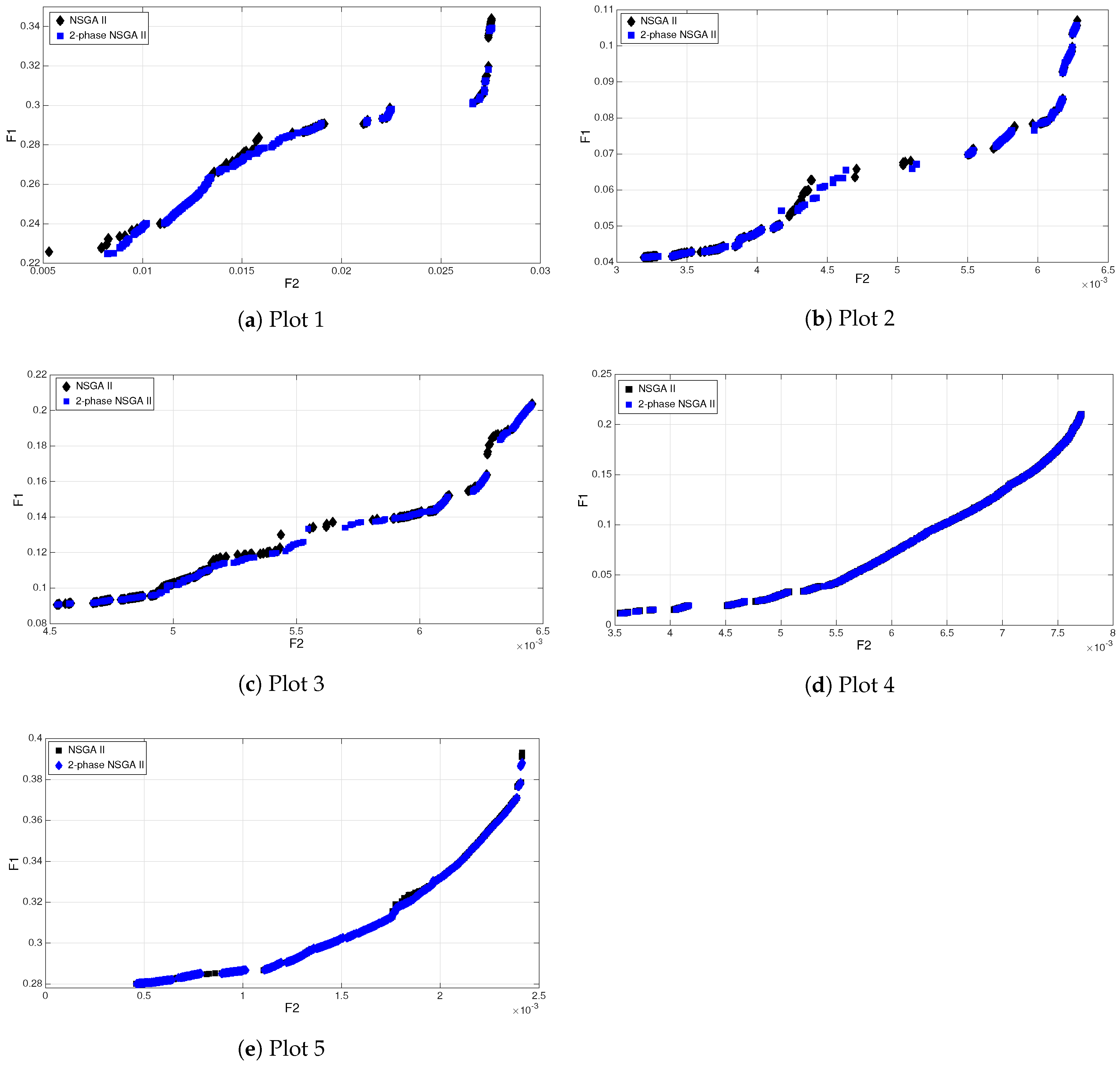
Each algorithm was performed ten times and all results of these ten runs were overlapped. Then, the non-dominated solutions were chosen. Figure 3 presents the non-dominated solutions of accumulated runs by NSGA II and 2-phase NSGA II for five test problems. As it can be seen, the introduced algorithm worked impressively in all problem sizes. The values obtained for all metrics for all test problems are shown in Table 4.
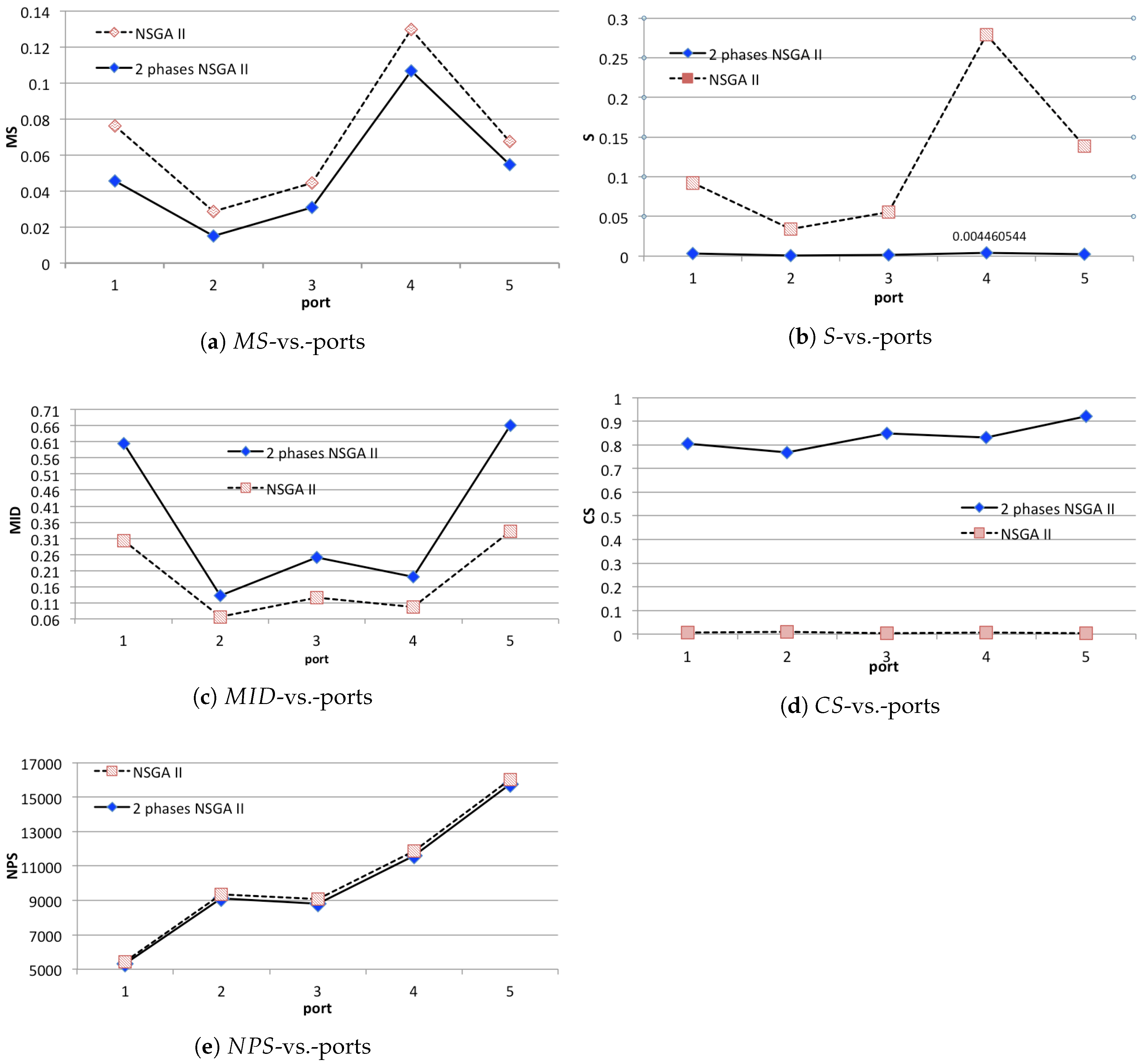
Obviously, according to S, C S and N P S criteria the 2-phase NSGA II acquired better results than NSGA II, meanwhile based on M I D and M S factors there are not any clear differences between the two algorithms.

Analysis of the Results

We used non-parametric statistical test of Mann-Whitney to analyze the outputs of the algorithms. P v a l u e of each metric for all five test problems is represented in Table 5, according to which no significant differences were observed between the two algorithms based on MID and MS metrics while the significant differences between the two algorithms was clear according to N P S , S and C S .
Also, Figure 4 shows means plot for the interaction among the metrics of algorithm and test problems. As can be seen, the proposed algorithm has generally better performance based on S, C S and N P S metrics. According to M I D and M S metrics, the graphs of both algorithms are very close to each other.

6. Conclusions and Future Developments

In the present work, the problem of portfolio optimization with bi-objectives of risk and reward is solved by Multi-objective Evolutionary Algorithms. These algorithms were necessary to be applied because of binary variable of δ i . 2-phase NSGA II algorithm was proposed and the results of this algorithm were compared with NSGA II algorithm. For statistical analysis Mann-Whitney test was used and the efficiency of the algorithms were validated by different comparison metrics (such as number of Pareto solutions, maximum spread of the solution set, spacing of the Pareto set, mean ideal distance, and coverage set). The proposed algorithm outperforms the NSGA II based on N P S , S and C S metrics while the difference between them is not significant according to M I D and M S factors.
We believe that there is an extensive area of improvement in the multi-phase heuristic algorithm and the proposed algorithm presented here is a good starting point for creating more efficient and robust algorithm. In the future, it is suggested to consider the proposed algorithm of 2-phase NSGA II on other optimization problems. Also it would be worthwhile to consider other objectives and constraints in the real world for the model and then investigate the performance of 2-phase NSGA II. Furthermore, the results could be compared with other heuristics algorithms.

Acknowledgments

Authors want to thank the editor and the reviewers for their valuable comments and suggestions that helped us to improve the quality of our paper. Also, they would like to thank Dr. Zahra Pooranian Research Associate at the University of Padova, Italy for her kind comments and advice.

Author Contributions

All authors together proposed, discussed and finalized the main idea of this work. Seyedeh Elham Eftekharian and Mohammad Shojafar proposed the idea and implemented the algorithm and their comparisons. Mohammad Shojafar and Shahaboddin Shamshirband calculated and plotted the feasible regions and helped in the paper preparations.

Conflicts of Interest

The authors declare no conflict of interest.

References

  1. Markowitz, H. Portfolio selection. J. Financ. 1952, 7, 77–91. [Google Scholar]
  2. Markowitz, H.M. Portfolio Selection: Efficient Diversification of Investments; Yale University Press: New Haven, CT, USA, 1968; Volume 16. [Google Scholar]
  3. Chang, T.J.; Meade, N.; Beasley, J.E.; Sharaiha, Y.M. Heuristics for cardinality constrained portfolio optimisation. Comput. Oper. Res. 2000, 27, 1271–1302. [Google Scholar] [CrossRef]
  4. Crama, Y.; Schyns, M. Simulated annealing for complex portfolio selection problems. Eur. J. Oper. Res. 2003, 150, 546–571. [Google Scholar] [CrossRef]
  5. Gilli, M.; Këllezi, E. A global optimization heuristic for portfolio choice with VaR and expected shortfall. In Computational Methods in Decision-Making, Economics and Finance; Springer: Berlin, Germany, 2002; pp. 167–183. [Google Scholar]
  6. Shojafar, M.; Cordeschi, N.; Baccarelli, E. Energy-efficient adaptive resource management for real-time vehicular cloud services. IEEE Trans. Cloud Comput. 2016, 99, 1–14. [Google Scholar] [CrossRef]
  7. Metawa, N.; Hassan, M.K.; Elhoseny, M. Genetic algorithm based model for optimizing bank lending decisions. Expert Syst. Appl. 2017, 80, 75–82. [Google Scholar] [CrossRef]
  8. Dueck, G.; Winker, P. New concepts and algorithms for portfolio choice. Appl. Stoch. Models Data Anal. 1992, 8, 159–178. [Google Scholar] [CrossRef]
  9. Celikyurt, U.; Özekici, S. Multiperiod portfolio optimization models in stochastic markets using the mean–variance approach. Eur. J. Oper. Res. 2007, 179, 186–202. [Google Scholar] [CrossRef]
  10. Allen, L.; Saunders, A. Incorporating systemic influences into risk measurements: A survey of the literature. J. Financ. Serv. Res. 2004, 26, 161–191. [Google Scholar] [CrossRef]
  11. Anagnostopoulos, K.; Mamanis, G. A portfolio optimization model with three objectives and discrete variables. Comput. Oper. Res. 2010, 37, 1285–1297. [Google Scholar] [CrossRef]
  12. Chiam, S.; Tan, K.; Al Mamum, A. Evolutionary multi-objective portfolio optimization in practical context. Int. J. Autom. Comput. 2008, 5, 67–80. [Google Scholar] [CrossRef]
  13. Duellmann, K.; Masschelein, N. A tractable model to measure sector concentration risk in credit portfolios. J. Financ. Serv. Res. 2007, 32, 55–79. [Google Scholar] [CrossRef]
  14. Pelusi, D.; Tivegna, M.; Ippoliti, P. Improving the profitability of technical analysis through intelligent algorithms. J. Interdiscip. Math. 2013, 16, 203–215. [Google Scholar] [CrossRef]
  15. Pelusi, D.; Mascella, R.; Tallini, L. Revised gravitational search algorithms based on evolutionary-fuzzy systems. Algorithms 2017, 10, 44. [Google Scholar] [CrossRef]
  16. Deng, G.F.; Lin, W.T.; Lo, C.C. Markowitz-based portfolio selection with cardinality constraints using improved particle swarm optimization. Expert Syst. Appl. 2012, 39, 4558–4566. [Google Scholar] [CrossRef]
  17. Lin, C.C.; Liu, Y.T. Genetic algorithms for portfolio selection problems with minimum transaction lots. Eur. J. Oper. Res. 2008, 185, 393–404. [Google Scholar] [CrossRef]
  18. Fernández, A.; Gómez, S. Portfolio selection using neural networks. Comput. Oper. Res. 2007, 34, 1177–1191. [Google Scholar] [CrossRef]
  19. Chang, T.J.; Yang, S.C.; Chang, K.J. Portfolio optimization problems in different risk measures using genetic algorithm. Expert Syst. Appl. 2009, 36, 10529–10537. [Google Scholar] [CrossRef]
  20. Yu, L.; Wang, S.; Lai, K.K. Neural network-based mean–variance–skewness model for portfolio selection. Comput. Oper. Res. 2008, 35, 34–46. [Google Scholar] [CrossRef]
  21. Cura, T. Particle swarm optimization approach to portfolio optimization. Nonlinear Anal. Real World Appl. 2009, 10, 2396–2406. [Google Scholar] [CrossRef]
  22. Chen, W.; Zhang, W.G. The admissible portfolio selection problem with transaction costs and an improved PSO algorithm. Phys. A Stat. Mech. Appl. 2010, 389, 2070–2076. [Google Scholar] [CrossRef]
  23. Soleimani, H.; Golmakani, H.R.; Salimi, M.H. Markowitz-based portfolio selection with minimum transaction lots, cardinality constraints and regarding sector capitalization using genetic algorithm. Expert Syst. Appl. 2009, 36, 5058–5063. [Google Scholar] [CrossRef]
  24. Ong, C.S.; Huang, J.J.; Tzeng, G.H. A novel hybrid model for portfolio selection. Appl. Math. Comput. 2005, 169, 1195–1210. [Google Scholar] [CrossRef]
  25. Armananzas, R.; Lozano, J.A. A Multiobjective Approach to the Portfolio Optimization Problem. In Proceedings of the IEEE 2005 IEEE Congress on Evolutionary Computation, Edinburgh, Scotland, 2–5 September 2005; pp. 1388–1395. [Google Scholar]
  26. Diosan, L. A Multi-Objective Evolutionary Approach to the Portfolio Optimization Problem. In Proceedings of the IEEE International Conference on Computational Intelligence for Modelling, Control and Automation and International Conference on Intelligent Agents, Web Technologies and Internet Commerce (CIMCA-IAWTIC’06), Vienna, Austria, 28–30 November 2005; Volume 2, pp. 183–187. [Google Scholar]
  27. Subbu, R.; Bonissone, P.P.; Eklund, N.; Bollapragada, S.; Chalermkraivuth, K. Multiobjective Financial Portfolio Design: A Hybrid Evolutionary Approach. In Proceedings of the 2005 IEEE Congress on Evolutionary Computation, Edinburgh, UK, 2–5 September 2005; Volume 2, pp. 1722–1729. [Google Scholar]
  28. Branke, J.; Scheckenbach, B.; Stein, M.; Deb, K.; Schmeck, H. Portfolio optimization with an envelope-based multi-objective evolutionary algorithm. Eur. J. Oper. Res. 2009, 199, 684–693. [Google Scholar] [CrossRef]
  29. Lwin, K.; Qu, R.; Kendall, G. A learning-guided multi-objective evolutionary algorithm for constrained portfolio optimization. Appl. Soft Comput. 2014, 24, 757–772. [Google Scholar] [CrossRef]
  30. Hallerbach, W.G.; Spronk, J. The relevance of MCDM for financial decisions. J. Multi-Criteria Decis. Anal. 2002, 11, 187–195. [Google Scholar] [CrossRef]
  31. Pindoriya, N.; Singh, S.; Singh, S. Multi-objective mean–variance–skewness model for generation portfolio allocation in electricity markets. Electr. Power Syst. Res. 2010, 80, 1314–1321. [Google Scholar] [CrossRef]
  32. Jana, P.; Roy, T.; Mazumder, S. Multi-objective mean-variance-skewness model for portfolio optimization. Adv. Model. Optim. 2007, 9, 181–193. [Google Scholar]
  33. Abdelaziz, F.B.; Aouni, B.; El Fayedh, R. Multi-objective stochastic programming for portfolio selection. Eur. J. Oper. Res. 2007, 177, 1811–1823. [Google Scholar] [CrossRef]
  34. Lo, A.W.; Petrov, C.; Wierzbicki, M. It’s 11 p.m.—Do you know where your liquidity is? The mean-variance-liquidity frontier. World Risk Manag. 2003, 1, 47. [Google Scholar]
  35. Yakut, E.; Çankal, A. Portfolio Optimzation Using of Metods Multi Objective Genetic Algorithm and Goal Programming: An Application in BIST-30. Bus. Econ. Res. J. 2016, 7, 43–62. [Google Scholar] [CrossRef]
  36. Deb, K.; Pratap, A.; Agarwal, S.; Meyarivan, T. A fast and elitist multiobjective genetic algorithm: NSGA-II. IEEE Trans. Evol. Comput. 2002, 6, 182–197. [Google Scholar] [CrossRef]
  37. Anagnostopoulos, K.P.; Mamanis, G. Multiobjective evolutionary algorithms for complex portfolio optimization problems. Comput. Manag. Sci. 2011, 8, 259–279. [Google Scholar] [CrossRef]
  38. Behnamian, J.; Ghomi, S.F.; Zandieh, M. A multi-phase covering Pareto-optimal front method to multi-objective scheduling in a realistic hybrid flowshop using a hybrid metaheuristic. Expert Syst. Appl. 2009, 36, 11057–11069. [Google Scholar] [CrossRef]
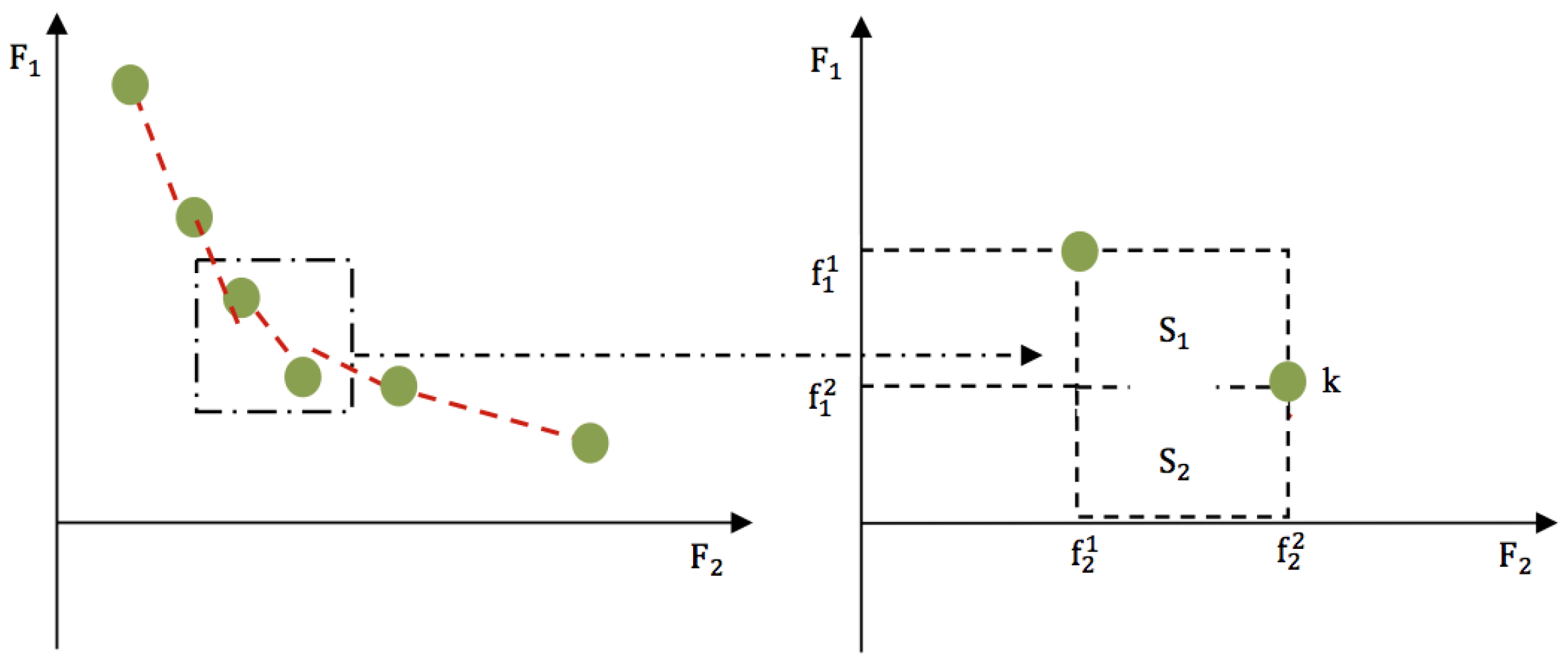
Figure 1. Selecting two adjacent solutions in the second phase of 2-phase NSGA II algorithm.
Algorithms 10 00130 g001
Figure 2. The covering and improvement of the Pareto-front in two runs.
Algorithms 10 00130 g002
Figure 3. Pareto-front of non-dominated solutions yielded by both algorithms for five test problems.
Algorithms 10 00130 g003
Figure 4. Pareto-front of non-dominated solutions yielded by both algorithms for five test problems.
Algorithms 10 00130 g004
Table 1. Data set characteristics.
Problem IndexData SourceNumber of Assets
Port 1Hong Kong, hang seng31
Port 2German, Dax 10085
Port 3British, FTSE 10089
Port 4US, S&P 10098
Port 5Japanese, Nikkei 225225
Table 2. Metrics formula.
MetricFormula
MID i = 1 N C i N , C i = ( f i 1 f 0 1 ) 2 ( f i 2 f 0 2 ) 2
MS m = 1 M i = 1 | Q | max f m i min f m i 2
S 1 | Q | i = 1 | Q | d i d ¯ 2
CS C ( A , B ) = | { b B | a A : a b } | | B |
Table 3. Distinguished parameters for each problem size.
Problems NoG popsize kM
Port 1400100108
Port 25002002017
Port 33002002018
Port 45002002014
Port 53002003023
Table 4. Evaluation of non-dominated solution.
Problem Size Algorithm and Index
MIDNPS
PortNNSGA II2-p NSGA IINSGA II2-p NSGA II
Port 1310.283430.274332736481
Port 2850.074280.07281145151,032
Port 3890.135280.1381135843,487
Port 4980.102340.101167836,348
Port 52250.316020.3136574249,061
MSS
PortNNSGA II2-p NSGA IINSGA II2-p NSGA II
Port 1310.120250.116230.200620.01591
Port 2850.065740.064530.068870.00284
Port 3890.11320.112760.159460.0056
Port 4980.198750.198480.343570.00777
Port 52250.316020.313650.222090.00558
C
PortNNSGA II2-p NSGA II
Port 1310.006940.80952
Port 2850.018130.77739
Port 3890.035070.8947
Port 4980.016180.82006
Port 52250.018610.90701
Table 5. Mann-Whitney analysis for each metric.
Metricp-Value
MID0.852
NPS0.000
MS0.027
S0.000
CS0.000