Article

Local Community Detection in Dynamic Graphs Using Personalized Centrality †

School of Computational Science and Engineering, Georgia Tech, Atlanta, GA 30332, USA
*
Author to whom correspondence should be addressed.
This paper is an extended version of our paper published in ICCS 2017, ASONAM 2017, and GABB 2016.
Algorithms 2017, 10(3), 102; https://doi.org/10.3390/a10030102
Submission received: 31 May 2017 / Revised: 22 August 2017 / Accepted: 23 August 2017 / Published: 29 August 2017
(This article belongs to the Special Issue Algorithms for Community Detection in Complex Networks)

Abstract

:
Analyzing massive graphs poses challenges due to the vast amount of data available. Extracting smaller relevant subgraphs allows for further visualization and analysis that would otherwise be too computationally intensive. Furthermore, many real data sets are constantly changing, and require algorithms to update as the graph evolves. This work addresses the topic of local community detection, or seed set expansion, using personalized centrality measures, specifically PageRank and Katz centrality. We present a method to efficiently update local communities in dynamic graphs. By updating the personalized ranking vectors, we can incrementally update the corresponding local community. Applying our methods to real-world graphs, we are able to obtain speedups of up to 60× compared to static recomputation while maintaining an average recall of 0.94 of the highly ranked vertices returned. Next, we investigate how approximations of a centrality vector affect the resulting local community. Specifically, our method guarantees that the vertices returned in the community are the highly ranked vertices from a personalized centrality metric.

1. Introduction

A variety of applications from many different fields of research, such as society, network security, finance, and biology, represent their data in graphs. Broadly speaking, a graph is a collection of vertices and edges, where an edge between vertices represents a relationship between the two vertices. For example, in a social network, the vertices represent people and an edge between two people signifies a friendship or interaction between them. In a financial network, the vertices may also be people but an edge between two people may indicate that these two people participated in a mutual transaction. Much of real data today changes constantly, so we turn to dynamic graphs. Dynamic graph data represents the changing relationships between different entities over time.
Two fundamental topics in the analysis of large, dynamic graphs are (1) identifying closely related subgraphs or communities, and (2) measuring vertex “importance” or centrality. Community detection identifies groups of vertices more closely related to each other than to the rest of the graph. In a social network, a community may represent a group of friends or people who share a similar interest. In a financial network, a community may be a group of people who regularly participate in transactions with each other. Global community detection methods partition the entire graph into different communities. Typically, most methods partition the graph into disjoint communities, but overlapping community detection is also a growing field of research. In contrast to global community detection methods that seek to optimize a global partition on the graph, local community detection methods aim to identify a single community in the graph relevant to a few seed vertices of interest. This problem is alternatively called seed set expansion. Since many real graphs have millions or billions of vertices or edges, visualization is extremely difficult. Furthermore, many computationally intensive algorithms cannot be run on such large graphs. Seed set expansion can be used to extract a smaller, relevant subgraph for further analysis.
In addition to community detection, identifying the most important vertices in a graph is another well-studied problem in network analysis. In a social network, these might be the people who are the most influential on a social networking site. In a network modeling disease spread, these might be the sites of disease origin. To identify vertex importance, we use centrality measures, which assign a numerical score to each vertex in the graph. These numerical scores can then in turn be translated into rankings on the vertices of the graph, where highly ranked vertices are the most “important” vertices in the graph. We can again think of centrality in terms of global values or local values. Intuitively, global centrality values indicate how important each vertex is with respect to all other vertices. In contrast, local centrality values (or personalized centrality) indicate how important vertices are with respect to specific seed vertices of interest. In this work, we bridge the two research questions of community detection and centrality by using personalized centrality metrics to identify local communities in dynamic graphs.

1.1. Contributions

This paper’s contributions along with main results and the sections in which they appear are presented in Table 1.
We extend our previous work in [1,2,3] by applying it to the problem of local community detection, defined further in Section 3.1. Our work on updating PageRank and Katz Centrality are necessary steps towards tracking “relevant” subgraphs around seed vertices using personalized centrality metrics. Specifically, the main contribution of this paper is to tie together the two fields of community detection and centrality by studying how personalized centrality metrics can be used for local community detection in not only static but also dynamic graphs.
The remainder of the article is organized as follows. Section 2 provides background and definitions. We review relevant literature regarding community detection and centrality metrics in Section 3. Section 4’s preliminary results include initial validation of our method on static graphs. The algorithms for application to dynamic graphs as well as a thorough discussion of experiments and results appear in Section 5. Section 6 presents the theoretical guarantees relating an approximation to the exact centrality metric with experimental validation. Finally, we conclude and discuss future research directions in Section 7.

2. Background

2.1. Definitions

Let G = ( V , E ) be a graph, where V is the set of n vertices and E the set of m edges. Denote the n × n adjacency matrix A of G as
A ( i , j ) = 1 , if ( i , j ) E , 0 , otherwise .
We use undirected, unweighted graphs so i , j , A ( i , j ) = A ( j , i ) and all edge weights are 1. Algorithms can apply the linear operator in A by traversing the graph G without constructing a matrix. Much real data today is constantly changing, requiring support for dynamic graphs. We can think of a dynamic graph representation as a series of snapshots of the graph G taken at different points in time t. We denote the current snapshot of the dynamic graph G and corresponding adjacency matrix A at time t by G t = ( V t , E t ) and A t , respectively. In this work, the vertex set is constant over time so t , V t = V . Our algorithms handle both edge insertions and deletions. Given edge updates to the graph, we can write the new adjacency matrix at time t + 1 as A t + 1 = A t + Δ A , where Δ A represents the new edges being added to (or removed from) the graph.
To reduce subscripts slightly, each change prefixed by Δ is associated with time t.
We represent a community C in the graph as a group of vertices { v 1 , v 2 , , v | C | } .

2.2. Measures of Community Quality

Since there is no universal definition of a community, there are several metrics that exist to evaluate the quality of a community. Several of these metrics focus on calculating how tightly knit a community is in terms of comparing the number of inter-community edges to the number of intra-community edges. Let k i n C denote the number of intra-community edges for community C; that is, the number of edges ( i , j ) with both endpoints vertex i and j inside the community. Similarly, let k o u t C denote the number of inter-community edges, or the number of edges ( i , j ) where vertex i is in the community and vertex j is outside the community. Conductance ( ϕ ) is a popular measure for measuring the “fitness” of a community by measuring the community cut, or the inter-community edges. Conductance is calculated as
ϕ ( C ) = k o u t C m i n ( 2 k i n C + k o u t C , 2 k i n V C + k o u t V C )
in [4]. When optimizing a community with respect to conductance, we seek to minimize conductance scores. A lower conductance score indicates a more tightly knit community. Another popular metric for evaluating the quality of communities is to calculate a modified ratio of intra- to inter-community edges, or a normalized edge cut (f) [5] as
f ( C ) = 2 k i n C + 1 2 k i n C + k o u t C .
Here, a larger value of the normalized edge cut indicates a more tightly knit community, so methods that optimize for the value of the normalized edge cut of a community seek to maximize f ( C ) . Modularity (Q) compares the number of intra-community edges to the expected number under a random null model and is calculated as
Q ( C ) = k i n C ( 2 k i n C + k o u t C ) 2 4 | E |
in [6]. Again, larger values of modularity indicate higher quality communities so algorithms optimizing for modularity seek to maximize values of modularity. Several other metrics were used in recent DIMACS (Center for Discrete Mathematics and Theoretical Computer Science) challenges: the intra-cluster density is defined as k i n / ( | C | 2 ) and converage of a community is calculated as k i n / | E | . For a more detailed list of metrics to measure community quality, see [7].

2.3. Centrality Measures

As mentioned earlier, identification of the most “important” vertices in graphs is a fundamental problem in network analysis, which is done using centrality measures. In this work, we focus on two popular linear algebra based metrics, Katz centrality and PageRank, that can be written as functions of the adjacency matrix A.
Katz centrality scores ( c K a t z ) count the number of weighted walks in a graph starting at vertex i, penalizing longer walks with a user-chosen parameter α , where α ( 0 , 1 / A 2 ) [8]. A walk in a graph traverses edges between a series of vertices v 1 , v 2 , , v k , where vertices and edges are allowed to repeat. To count weighted walks of different lengths in the graph, we sum powers of the adjacency matrix [9] using the infinite series
k = 1 α k 1 A k = A + α A 2 + α 2 A 3 + α 3 A 4 + + α k 1 A k + ,
where A k ( i , j ) is the number of walks of length k from vertex i to vertex j. Provided α is chosen to be within the appropriate range, this infinite series converges to the matrix resolvent A ( I α A ) 1 , where I is the n × n identity matrix. When Katz centrality was first introduced, Katz used the column sums to calculate vertex importance to obtain centrality scores as A ( I α A ) 1 1 , where 1 is the n × 1 vector of all 1s. These are referred to as global Katz scores and count the total sum of the number of weighted walks of different length starting at each vertex. We can extrapolate from this definition personalized Katz scores, where the ith column of the matrix A ( I α A ) 1 represents the personalized scores with respect to vertex i, or the weighted counts of the number of walks from vertex i to all other vertices in the graph. Mathematically, we can write the personalized Katz scores with respect to vertex i as A ( I α A ) 1 e i , where e i is the ith canonical basis vector, the vector of all 0s except a 1 in the ith position. If we desire personalized scores with respect to a seed set of vertices S = { v 1 , v 2 , v | S | } , we define the vector e S = e v 1 + e v 2 + + e v | S | and calculate the scores as A ( I α A ) 1 e S . In this work, we deal only with personalized centrality scores. To summarize, we denote the centrality scores obtained through Katz centrality as the n × 1 vector c K a t z = A ( I α A ) 1 e i . If we let M K a t z = I α A , then we can first solve the linear system M K a t z x K a t z = b K a t z for x K a t z and then obtain the personalized centrality scores as c K a t z = A x K a t z .
PageRank is another walk-based centrality metric that assigns high scores to vertices that are visited by a large number of random walks in the network [10]. We can also write PageRank scores ( c P R ) as a function of the adjacency matrix A, as c P R = ( I α A T D 1 ) 1 b P R , where here α is known as the “teleportation” constant and v is a personalization vector with v 1 = 1. Similar to Katz centrality, we can define global and personalized scores. If v has entries 1 / | V | denoting a uniformly random start, we obtain global scores, otherwise for personalized scores w.r.t. vertex i we can set v = e i . Again if we desire personalized scores with respect to a seed set of vertices S = { v 1 , v 2 , v | S | } , we define the normalized vector e S = ( e v 1 + e v 2 + + e v | S | ) / | S | and calculate the scores as A ( I α A ) 1 e S . If we let M P R = I α A T D 1 , then we can solve the linear system M P R c P R = b P R for c P R .
Since solving for many linear algebra based centrality measures directly is generally intractable, in practice, we use iterative solvers to solve them [11]. Iterative methods approximate the solution x in a linear system M x = b , given M and b . The iterative method we use in this work is the Jacobi method [12] given in Algorithm 1, although the work applies to other iterative techniques. At each iteration k of the iterative solver, we obtain new approximations x ( k ) and c ( k ) to the unknown exact solutions x * and c * , respectively. The error at each iteration is denoted as the difference between the exact and approximation, x * x ( k ) 2 and the residual norm as r k = b M x ( k ) 2 , where · 2 denotes the 2-norm. In practice, as the exact solution is not known, typical stopping criteria for the iterative solver is that the solution has not changed much. With Jacobi iteration, this is equivalent to terminating once the residual norm is below the input convergence threshold.
Algorithm 1 Solve M x = b to tolerance t o l using Jacobi algorithm.
  1:procedure Jacobi( M , b , t o l )
  2:k = 0
  3: x ( 0 ) = 0
  4: r ( 0 ) = b M x ( 0 )
  5: D = d i a g ( M )
  6: R = M D
  7:while r ( k ) 2 > t o l do
  8:   x ( k + 1 ) = D 1 ( R x ( k ) + b )
  9:   r ( k + 1 ) = b M x ( k + 1 ) ▹ Next residual
10:   k + = 1
11:end while
12:return x ( k + 1 )
13:end procedure
Given a graph and its adjacency matrix A, we can solve the corresponding linear system for c P R (for PageRank) or c K a t z (for Katz centrality) for the centrality scores on vertices of the graph.

3. Related Work

3.1. Community Detection

Most of the literature in the field of community detection focuses on finding global communities in a static, unchanging graph. Popular methods include greedy agglomerative algorithms such as the Clauset-Newman-Moore (CNM) algorithm [13] and the Louvain method [14]. These two methods find a global partition of the graph in which each vertex belongs to exactly one community. Another widely used method of finding global, non-overlapping communities is spectral partitioning, which uses the eigenvectors of the Laplacian of the graph adjacency matrix to partition the graph in two [4,15]. This process may be repeated recursively to find smaller communities.
While much of previous work has focused on partitioning methods that find non-overlapping communities, there are many methods that identify overlapping clusters. These include clique percolation [16], label propagation [17,18], edge partitioning [19], Order Statistics Local Optimization Method (OSLOM) [20], multiple local expansions [5,21,22], and ensemble combinations [23].
Community detection has also been studied in the context of dynamic graph data and this work can be broadly divided into two categories. Algorithms in the first category focus only on quality, while those in the second aim to both detect high quality communities and minimize computation. Typically, methods in the former category seek to find the best sequence of communities given the dynamic data by maximizing both the quality of communities found at each point in time and the smoothness of community change over time. This can be done by collecting all temporal data before inferring communities, as in [24,25,26]. Using all temporal data may produce better choices of communities over time, but may be computationally expensive and can only be performed after all data is collected. Therefore, this approach is not suitable for applications in which updated communities must be found quickly. Alternatively, each community may be found using only past data, as in evolutionary clustering [27] and FaceNet [28].
In the other category of dynamic community detection work, the goal is to both maintain good communities on a changing graph while minimizing computation. Typically, this is done as follows. A graph is formed from an initial set of data and communities are identified. When the graph changes due to new data, new communities are found by starting with the previous community solution and incrementally updating it. Many algorithms of this type update the results of greedy, agglomerative algorithms. For example, Aynaud et al. [29] presents an incremental version of the Louvain algorithm. Whenever the graph changes, the previous clusters are used as a starting point. Changes are made by checking if the modularity would increase by moving any vertex to a different community. The work in [30] is another incremental version of Louvain clustering that starts with the previous cluster assignment modified based on the graph changes that occurred. The Modules Identification in Evolving Networks algorithm (MIEN) [31] is an incremental version of greedy agglomerative methods such as CNM. In the work by Riedy and Bader, whenever edges are inserted or deleted, the endpoint vertices of such edges are moved from their communities into singleton communities before restarting their agglomerative algorithm [32]. In the work in [33] by Görke et al., the authors present algorithms to maintain a clustering of a dynamic graph where edges appear as a stream by optimizing modularity while guaranteeing smoother clustering dynamics. Our work falls into this second category of dynamic community detection, except that we deal with local communities, which are described next.
Local community detection is the task of finding the best community for a set of vertices of interest, often called seed vertices. This is also called seed set expansion. When dealing with massive graphs, running computationally intensive analytics, visualization, and manual inspection by human analysts is likely to be infeasible, and this difficulty only increases for dynamic data. In such cases, local community detection can be used to extract a smaller, relevant subgraph in order to perform such tasks. Clauset presented a greedy algorithm that starts with all seed vertices in the community and repeatedly checks all neighboring vertices for inclusion [34]. At each iteration, the neighboring vertex that most increases the chosen fitness score is added to the community. This method is shown in Algorithm 2, where C represents the community and N b ( C ) is the set of vertices neighboring C, or those with an edge to a vertex in C. In order to grow a community of k vertices, not including any seeds, it is necessary to perform k iterations and in each iteration check each neighboring vertex. Therefore, the complexity depends on the number of vertices bordering the community. This number may be approximated by k d , where d is the average degree of the graph and k the community size. In this case, the time complexity is given by O ( k 2 d ) . However, this is an overestimate when community members share many common neighbors, such as in graphs with a high clustering coefficient. In Section 4, we use synthetic, static graphs to compare the results of our method to this greedy seed set expansion algorithm. We show that our centrality based approach produces high quality communities compared to a common greedy approach and we explain when our approach is faster and preferable.
Finally, there has been some work in relating centrality measures and community detection, though much of the previous work has focused on the global or static case. Betweenness centrality as a measure of vertex importance was originally introduced by Freeman in [35] to measure influence of a vertex over the flow of information between other nodes by counting shortest paths in a network. The works by Girvan and Newman [6,36] extend the definition of vertex betweenness centrality to define edge betweenness as the number of shortest paths between pairs of vertices that run along it. Assuming communities in graphs are connected by only a few inter-community edges, these edges will have high edge betweenness. Therefore, by iteratively removing edges with the highest edge betweenness, community structure can be uncovered. A greedy local community algorithm using centrality metrics is the L-shell method [37], in which vertices are added to the community from successive shells, or sets of vertices at a fixed distance from the seed vertex. PageRank-Nibble is a spectral method of finding local communities in which personalized PageRank scores are computed and the community is formed by adding vertices with the highest values [38]. Our work differs from these previous works because we incrementally update scores to perform dynamic local community detection.
Section 5.3 compares our results with static expansion using Katz centrality in the place of PageRank.
Algorithm 2 Static, Greedy Seed Set Expansion
  1:procedure GreedySeedset(graph G, seed set s e e d )
  2: C = s e e d
  3: p r o g e s s = T r u e
  4:while p r o g r e s s do
  5:   m a x s c o r e = 1
  6:   m a x v t x = n u l l
  7:  for v N b ( C ) do
  8:    s ( v ) = f i t ( C v ) f i t ( C )
  9:   if s ( v ) > m a x s c o r e then
10:     m a x s c o r e = s ( v )
11:     m a x v t x = v
12:   end if
13:  end for
14:  if maxscore > 0 then
15:    C = C m a x v t x
16:  else
17:    p r o g e s s = f a l s e
18:  end if
19:end while
20:return C
21:end procedure

3.2. Dynamic Algorithms for Centrality Measures

While much of the literature tends to focus on optimizing algorithms for centrality measures on static graphs, a growing body of work addresses dynamic algorithms for updating centrality measures given updates to the underlying graph. As PageRank is one of the most commonly studied problems in the literature, we outline several dynamic algorithms for updating the centrality metric given edge updates to the graph. There are two general areas of techniques used to approximate dynamic updates to the PageRank vector: (1) linear algebraic methods that mainly use techniques from linear and matrix algebra and perhaps using some structural properties of the network [39,40], and (2) Monte Carlo methods that use a small number of simulated random walks per vertex to approximate PageRank [41,42]. Many linear algebraic techniques use “aggregation” methods, which operate under the assumption that changes to the underlying network affect only a localized portion of the PageRank vector [43,44]. Aggregation methods partition the set of vertices into two disjoint sets S and V \ S , where S is the set of all vertices close to the incremental change and V \ S is the set of all other vertices. All the vertices in V \ S are aggregated into a single hyper-vertex and a smaller graph is created. The PageRank values of all the vertices are updated using this smaller graph and the result is pushed back to the original graph. However, most aggregation techniques do not translate well for real-time applications due to both performance and quality reasons. Since the performance of these methods depends on the partitioning of the network, a poor partitioning can cause these methods to be extremely slow [45]. In terms of quality, since the aggregation is ultimately an approximation of the updated PageRank vector given incremental changes to the graph, the approximation error could potentially accumulate over time leading to a very poor quality PageRank vector. Monte Carlo methods for the incremental computation of approximate PageRank, personalized PageRank and similar random walk methods is examined in detail in [46]. These methods are typically very efficient and can achieve good quality personalized scores, but most literature on these approaches has thus far only been applied to static networks. These methods maintain a small number of short random walk segments starting at each vertex in the graph. For the case of identifying the top k vertices, these methods are able to provide highly accurate estimates of the centrality values for the top vertices, but smaller values in the personalized case are nearly identical and therefore impossible to tell apart. In [3], we present an algorithm for updating PageRank values in dynamic graphs by only using sparse updates to the residual is presented. A similar algorithm for updating Katz centrality scores is given in [2].
These two methods are the base for this work. We believe a similar method will apply to non-backtracking variants of Katz centrality [47] as well, but that remains as future work.
Personalized PageRank vectors and conductance scores have also been used to identify communities in graphs [48]. This method is based off of the fact that the personalized PageRank vector is the stationary distribution of a random walk that follows an edge of the graph with probability α and “teleports” back to the seed vertex with probability 1 α . The PageRank scores are calculated by an algorithm that pushes scores to neighboring vertices at each stage using the algorithm described in [38]. Once the PageRank vector is calculated, the algorithm performs a sweep cut to identify the optimal community. This procedure sweeps over all cuts induced by the ordering of the personalized PageRank vector and chooses the best cut determined by conductance scores of the induced cuts.
The entire personalized PageRank matrix, formed with each column starting from the corresponding vertex, has been shown asymptotically to recover the stochastic block model used here as a test case [49].

4. Communities from Personalized Centrality

4.1. Local Communities from Personalized Centrality

Given a seed set of vertices of interest, we can calculate the personalized Katz or PageRank scores as c K a t z = A ( I α A ) 1 b K a t z or c P R = M P R 1 b P R , respectively, where M K a t z = I α A and M P R = I α A T D 1 with b K a t z and b K a t z are the corresponding right-hand sides as discussed in Section 2.3. If we want the personalized scores w.r.t. vertex i, then b K a t z = b P R = e i . Intuitively, the resultant scores from a personalized centrality metric with respect to vertex i answers the question of how likely we are to reach vertex i from the rest of the graph. For the question of local community detection, this can be translated into how likely vertices in the graph are to belong to the community of vertex i. For a community of size R, we therefore take the top R vertices as ranked by the personalized centrality vector c P R or c K a t z as the local community.
Once personalized Katz or PageRank centrality scores are computed, the local community is then formed from those vertices with highest centrality values. Sorting the entire length n vector to obtain these top entries is too computationally expensive, especially in the dynamic setting where updated results are needed quickly after changes occur. Therefore, we extract the vertices with top k values using a heap. For the first k vertices, the centrality values are added to a heap. Thereafter, each centrality score is compared to the minimum value in the heap in O ( 1 ) time and if larger, the minimum value is removed from and the new value inserted into the heap in O ( log k ) time. In the worst case, the centrality values are in ascending order and all such checks result in a removal and insertion, leading to a running time of O ( n log k ) . However, experiments on real graphs show far fewer replacements.

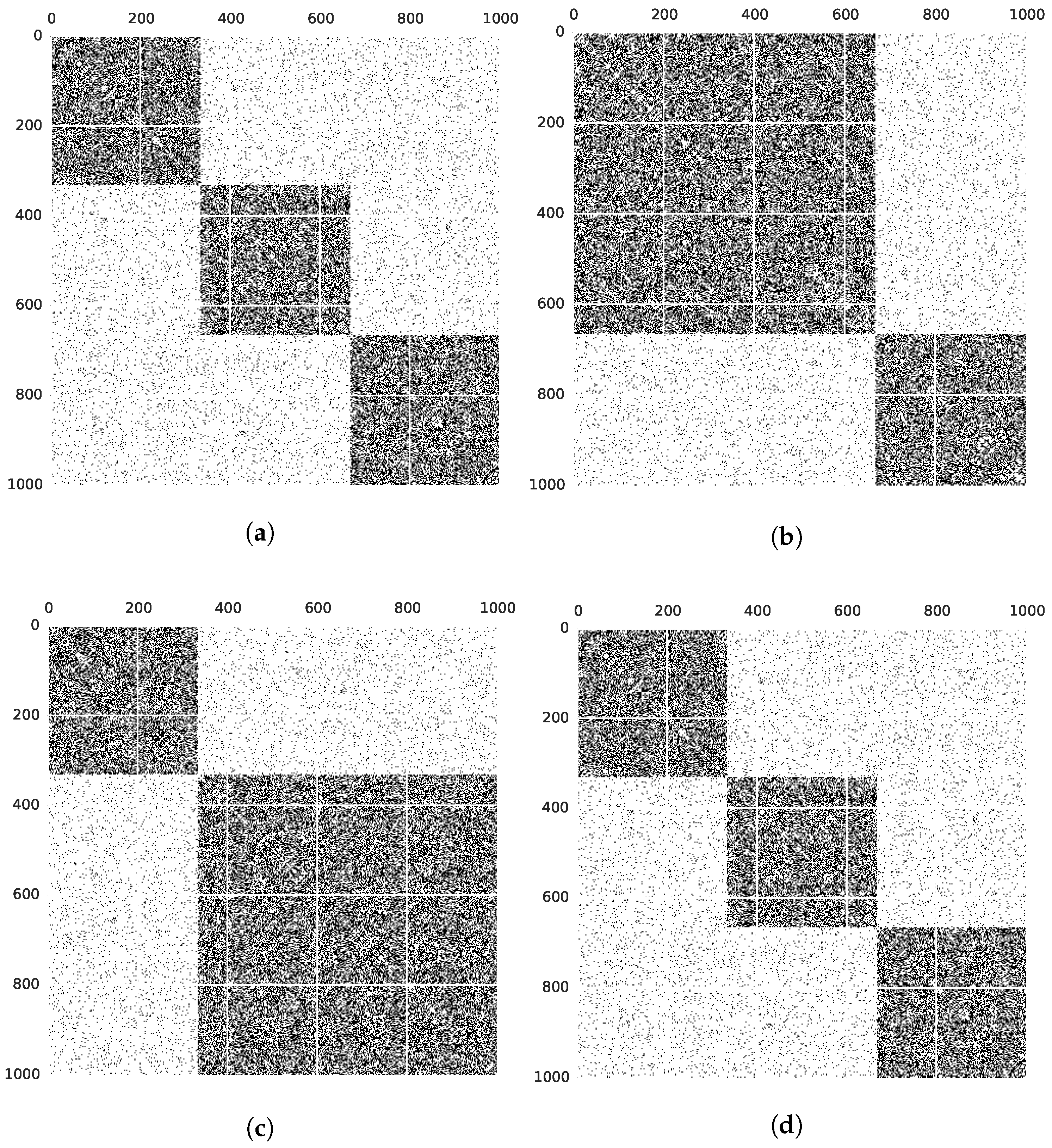
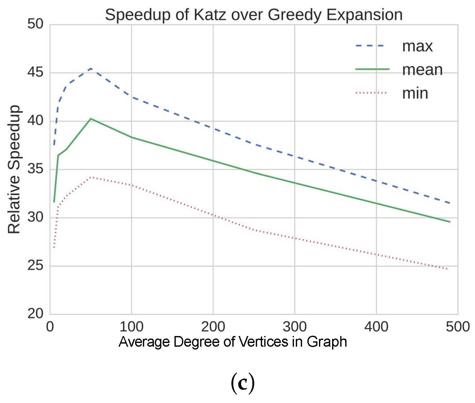
4.2. Results on Static, Synthetic Graphs

This section validates using personalized centrality for local community detection. Static, synthetic graphs with known community structure provide test cases for the Katz centrality approach. We also compare our approach to the popular method of greedy expansion [34], which is described in Section 3.1. To test, we generate multiple stochastic block model (SBM) graphs with varying parameters, randomly choose seed vertices, and detect local communities with both personalized Katz centrality and greedy expansion.
The greedy expansion method uses conductance as its fitness function. A simple stochastic block model graph can be generated with four parameters: the total number of vertices n, the number of communities k, the average degree of vertices d, and the percentage of inter-community edges ρ . All communities in such a graph are generated with the same parameters and are interchangeable. Note that SBM graphs can also be generated with different parameters than we use. Instead of using an average degree and proportion of inter-community edges, the parameters p i n and p o u t can be used. These define the probabilities of placing and edge between a pair of vertices that are in the same community and between a pair in different communities, respectively. Although different parameters are used, these two models are the same when all communities are generated with the same parameters. The parameters are related as follows. For a set community size of c = n k , p i n = d ( 1 ρ ) c and p o u t = d ρ c ( k 1 ) . The code was implemented in Python and run on an 18 core Intel Xeon CPU at 2.10 GHz.
Table 2a–c shows the recall of communities found with each method compared to the known ground truth. The recall is the fraction of the ground truth recovered by each method. For these results, random stochastic block model graphs were created with 1000 vertices and two communities and a random seed was chosen. The minimum, mean, and maximum recall values shown are obtained from 100 runs, each with a random graph and seed vertex.
For the results shown in Table 2a, the average degree of vertices was varies from 5 to 490, while the proportion of inter-community edges is fixed at 0 . 01 . All others are intra-community edges. Because the proportion is fixed, as the average degree increases, both the number of intra-community and inter-community edges increases. Overall, recall scores are at or near 1, showing that the Katz method returns good communities for all average degrees considered.
This suggests that using personalized centrality is a viable method of local community detection. In fact, on SBM graphs with low degrees, the personalized Katz method performs better than greedy expansion. This occurs because the greedy expansion method stops adding new vertices once a local quality maximum is reached. On very low degree SBM graphs, it stops expanding after adding only a few vertices, which results in very small communities and thus low recall. Therefore, we also show results for a modified version of the greedy algorithm in which expansion is forced to occur until the community reaches the desired size (labeled Force Expand in Table 2a–c). Normally, the greedy algorithm is not run in this way, but because we know the size of the community ahead of time, we can obtain these results. Note that results for the normal greedy algorithm and the forced expansion version tend to differ only for graphs in which the average degree is low compared to the community size.
Table 2b,c shows how the quality of communities detected varies for SBM graphs with an increasing proportion of inter-community edges. For these experiments, the average degree is fixed at 20 (Table 2b) and 100 (Table 2c), and the proportion of edges that are inter-community varies from 0 . 01 to 0 . 4 (thus the proportion of intra-community edges varies from 0 . 99 to 0 . 6 ). As the percentage of inter-community edges increases, the community structure becomes less defined, making community detection more difficult. As expected, all methods achieve the best recall for graphs with a low proportion of inter-community edges. For graphs with a lower average degree of 20, both the Katz and greedy expansion methods return high quality communities only when a small proportion of edges exist between communities. However, when the average degree is increased to 100, both methods are less sensitive to a large proportion of inter-community edges and achieve higher recall values. Overall, the quality of communities returned by the personalized Katz method is comparable to those returned by greedy expansion. While the mean recall is sometimes lower, the minimum recall tends to be higher, making the results more consistent. Note that both the standard greedy and forced expansion greedy algorithms can return communities with very low recall. This may occur if the standard greedy method stops expanding too early or if either version returns the wrong community. Because the method greedily maximizes conductance, if there is a single seed vertex, the next vertex added is its lowest degree neighbor. If this neighbor belongs to a different community, the algorithm may detect and return the wrong community.
An interesting phenomenon occurs in Table 2b for SBM graphs with degree 20 and 0 . 4 inter-community edges. The minimum recall obtained with greedy expansion increases compared to 0 . 3 inter-community edges. This reversal in trend occurs because, at 0 . 4 inter-community edges, the community structure is almost gone and the greedy algorithm returns an almost random set of vertices, including many correct vertices. For graphs with a stronger community structure, on the other hand, the minimum recall corresponded to cases in which the greedy algorithm did return a community, but not the correct one.
Next, we consider the relative running time of the personalized Katz approach compared to the greedy expansion method. Figure 1 plots the ratio running times, where a value of x greater than 1 indicates that the Katz method is x times faster than greedy expansion. For these tests, we also use static, synthetic SBM graphs. As before, graphs are generated with four different parameters: the total number of vertices, the number of communities, the average degree of vertices, and the percentage of inter-community edges. For each experiment, three of these parameters are held constant, while one is varied in order to isolate its effect on the running time. The results shown use the modified version of greedy expansion in which the algorithm is forced to expand to the desired community size. We used this version because for those SBM graphs with a very low average degree compared to community size, the standard greedy algorithm stopped expanding after only a few vertices, leading to small and incorrect communities (see Table 2). This is likely an artifact of the synthetic SBM graphs in which vertices have uniformly random degrees. For all plots in Figure 1, the proportion of inter-community edges ρ is set to 0 . 01 . Overall, we see that using the personalized Katz approach tends to be faster than running the greedy expansion method. Next, we discuss various ways in which the structure of a graph affects the relative running times.
In Figure 1a, speedup is shown for graphs with an increasing number of vertices, while the average degree is fixed at 20 and the number of communities is fixed at 2. This experiment shows that, with all other parameters held constant, the larger the number of vertices in the graph (and therefore the larger the community detected), the greater the speedup of using our Katz approach compared to greedy expansion. This occurs because the complexity of the greedy approach is approximately O ( c 2 d ) for a community size of c and average degree d, while the complexity of the Katz approach is O ( m ) for a graph with m edges.
The advantage of our centrality approach compared to greedy expansion is greatest when the size of the community is large relative to the total number of vertices. This can be seen in Figure 1b, where we vary the number of communities, while keeping the size of the graph constant at 47,104 vertices with an average degree of 20. It is clear that the speedup of the Katz method is greatest for the graphs with a small number of large communities. This occurs because the personalized Katz centrality computation is global and processes the entire graph, while greedy expansion processes only a local subgraph composed of the community and its one hop neighborhood. If, however, the community to be found is much smaller than the full graph, the greedy expansion method may be preferable.
Finally, we consider how the average vertex degree affects relative running times in Figure 1c. The number of vertices is held constant at 1000 with 2 communities. As the average degree increases, the speedup of the Katz method over greedy expansion first increases and then decreases. The increase in speedup occurs because a higher average degree results in larger community neighborhoods and the larger the neighborhood of the community is as it expands, the slower the greedy expansion is. However, once the average degree grows large enough, few or no new vertices are added to the neighborhood and the clustering coefficient of the graph simply increases. These results show that the running time advantage of the personalized Katz method compared to greedy expansion is greatest in graphs in which the community of interest has a large neighborhood and a low clustering coefficient.

5. Dynamic Communities from Personalized Centrality

5.1. Methods

We have detailed how to obtain a local community from a personalized centrality vector in Section 4.1. In this section, we describe how to obtain communities in dynamic graphs using personalized centrality metrics. The identification of local communities in dynamic graphs can be split into two components: (1) updating the personalized centrality vector every time the graph changes, and (2) obtaining the new local community from the updated centrality vector.
For both centrality metrics, if c t denotes the solution at time t, we solve for a correction Δ c so that we can obtain the new solution at time t + 1 as c t + 1 = c t + Δ c . Essentially, we use the old solution as a starting point for the new solution instead of recomputing from scratch each time the graph is changed.
Personalized Katz centrality scores w.r.t. vertex i are given as c K a t z = A x K a t z where x K a t z is the solution to the linear system ( I α A ) x K a t z = b K a t z for b K a t z = e i and personalized PageRank scores are given as c P R = ( I α A T D 1 ) 1 b P R , where c P R is the solution to the linear system ( I α A T D 1 ) c P R = b P R for c P R . After a batch of edge insertions to the graph, the static algorithm to obtain the updated Katz scores first recomputes x t + 1 , K a t z using an iterative solver and obtains c t + 1 , K a t z as A t + 1 x t + 1 , K a t z (for Katz centrality) or recomputes c t + 1 , P R (for personalized PageRank). For Katz centrality, since calculating c t given x t at any time point t is one matrix-vector multiplication and can be done in O ( m ) , this is not the bottleneck of static recomputation. Instead, the bottleneck is repeatedly updating x t , K a t z given more edges being inserted into the graph, and hence we focus our dynamic algorithm on limiting the number of iterations taken to obtain the updated vector x t , K a t z , and, similarly, for PageRank, the focus of our dynamic algorithm on limiting the number of iterations taken to obtain the updated vector c t , P R . Therefore, for Katz, we solve for the correction Δ x so that we can obtain the new solution at time t + 1 as x t + 1 = x t + Δ x . For PageRank, we solve for the correction Δ c so that we can obtain the new solution at time t + 1 as c t + 1 = c t + Δ c . The algorithm for updating Katz centrality is published in our previous work in [2] and the algorithm for updating PageRank is published in our previous work in [3].
The first step in updating the centrality vector is to measure how close the old solution x t , K a t z or c t , P R is to solving the system for the updated graph A t + 1 . We calculate the new residual for Katz centrality as r ˜ t + 1 , K a t z
r ˜ t + 1 , K a t z = b K a t z M t + 1 , K a t z x t , K a t z = b K a t z ( I α A t + 1 ) x t , K a t z = b K a t z x t , K a t z + α A t + 1 x t , K a t z = b K a t z x t , K a t z + α A t x t , K a t z α A t x t , K a t z + α A t + 1 x t , K a t z = r t , K a t z + α ( A t + 1 A t ) x t , K a t z = r t , K a t z + α Δ A x t , K a t z .
Similarly, for PageRank, we calculate the new residual as r ˜ t + 1 , P R (note since we use undirected graphs, A T = A ):
r ˜ t + 1 , P R = b P R M t + 1 , P R c t , P R = ( 1 α ) v c t , P R + α A t + 1 D t + 1 1 c t , P R = ( 1 α ) v c t , P R + α A D 1 c t , P R α A D 1 c t , P R + α A t + 1 D t + 1 1 c t , P R = r t , P R + α ( A t + 1 D t + 1 1 A D 1 ) c t , P R .
Note that, for both centrality measures, r ˜ t + 1 can be written in terms of the current residual at time t, edge updates Δ A , and the old solution. Next, we can use r ˜ t + 1 to set up a linear system for the correction Δ x or Δ c . We apply iterative refinement [50] and, for Katz centrality, solve the linear system
( I α A t + 1 ) Δ x = r ˜ t + 1 , K a t z = r t , K a t z + α Δ A x t , K a t z
for Δ x . For PageRank, we solve the linear system
( I α A t + 1 D t + 1 1 ) Δ c = r ˜ t + 1 , P R = r t , P R + α ( A t + 1 D t + 1 1 A D 1 ) c t , P R
for Δ c . Unlike iterative refinement’s typical use of a directly factored matrix, we rely on Jacobi iteration for solving the above systems.
The final step of our algorithm is to update the residuals r t + 1 , K a t z and r t + 1 , P R for the next time point. For Katz centrality, we can write the new residual r t + 1 , K a t z as
r t + 1 , K a t z = b K a t z ( I α A t + 1 ) x t + 1 , K a t z = b K a t z ( I α A t + 1 ) ( x t , K a t z + Δ x ) = b K a t z ( I α A t + 1 ) x t , K a t z ( I α A t + 1 ) Δ x = r ˜ t + 1 , K a t z ( I α A t + 1 ) Δ x = r t , K a t z + α Δ A x t , K a t z ( I α A t + 1 ) Δ x .
We can calculate Δ r , the difference in the two residuals at time t and t + 1 as Δ r = α Δ A x t , K a t z ( I α A t + 1 ) Δ x . Likewise, updating the residual for PageRank is very similar. We can write the new residual r t + 1 , P R as
r t + 1 , P R = ( 1 α ) v ( I α A t + 1 D t + 1 1 ) ( c t , P R + Δ c ) = ( 1 α ) ( I α A t + 1 D t + 1 1 ) c t , P R ( I α A t + 1 D t + 1 1 ) Δ c = r ˜ t + 1 , P R ( I α A t + 1 D t + 1 1 ) Δ c = r t , P R + α ( A t + 1 D t + 1 1 A t D t 1 ) c t , P R ( I α A t + 1 D t + 1 1 ) Δ c .
Then, we can calculate Δ r , the difference in the two residuals at time t and t + 1 as Δ r = α ( A t + 1 D t + 1 1 A t D t 1 ) c t , P R ( I α A t + 1 D t + 1 1 ) Δ c . Updating the residual comes with the potential issue of accumulating error over long periods of time. However, these cases are rare, and, for our purposes, we obtain accurate results using our methods compared to a pure static recomputation. In Section 5.2 and Section 5.3, we show that our algorithm for dynamic Katz centrality maintains good quality of the updated scores and provides significant speedup compared to a pure static recomputation in Section 5.3.

5.2. Synthetic Dynamic Graphs
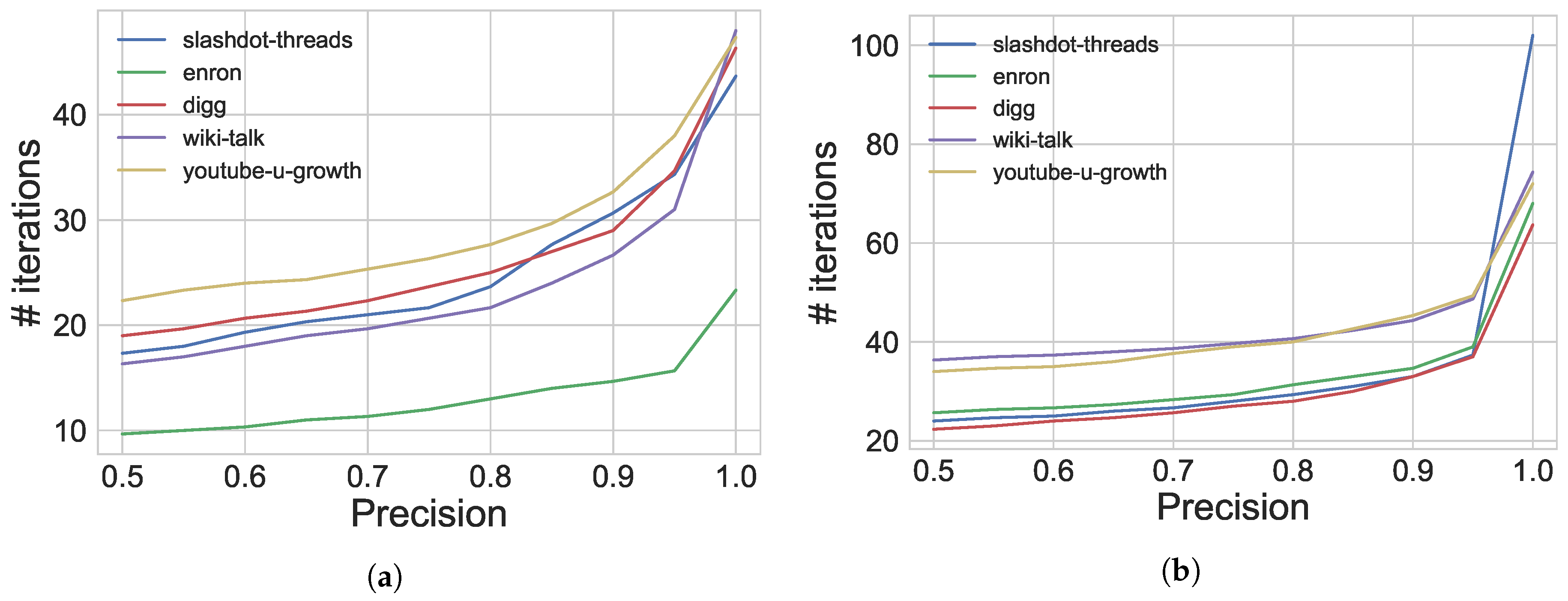
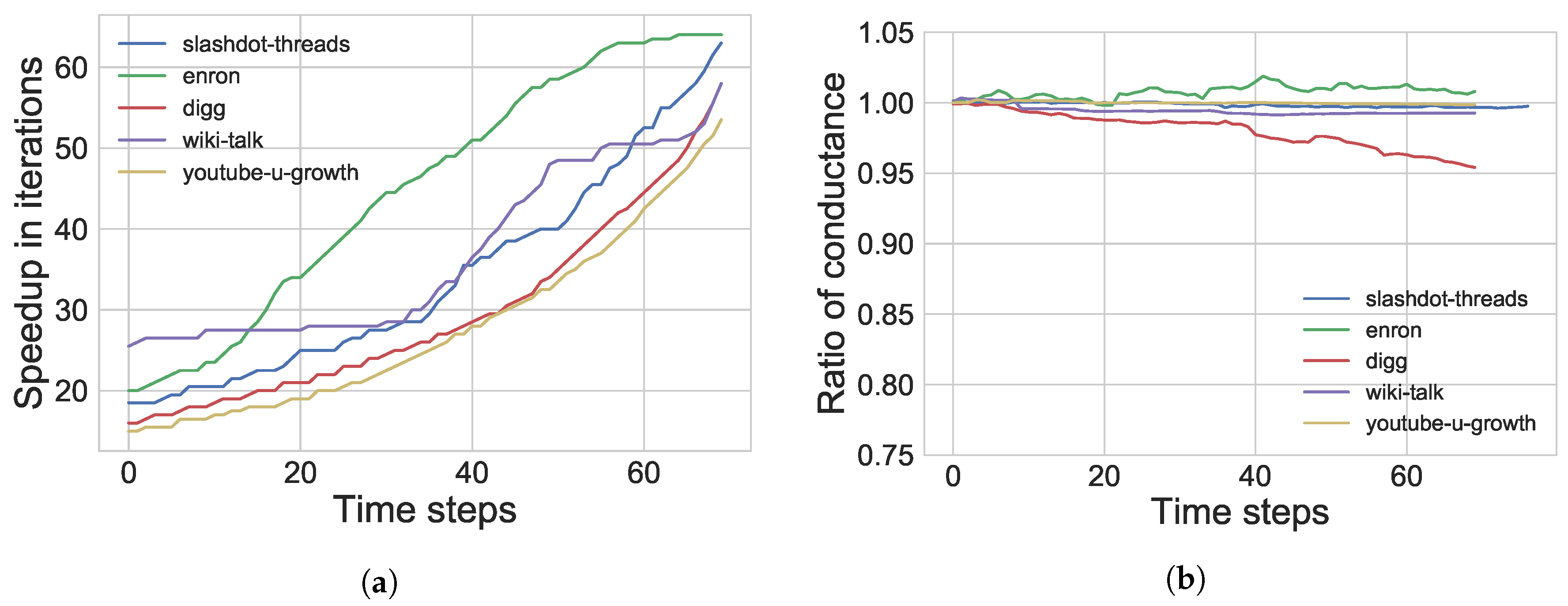
In this section, we evaluate our dynamic algorithm on a synthetic network to show our ability to track merging and splitting of communities. We use a synthetic stochastic block model network with a recursive matrix (R-MAT) background with parameters a = 0 . 55 , b = 0 . 15 , c = 0 . 15 , d = 0 . 25 . An R-MAT generator [51] creates scale-free networks designed to emulate real-world networks. Consider an adjacency matrix: the matrix is subdivided into four quadrants, where each quadrant has a different probability of being selected. Once a quadrant is selected, this quadrant is recursively subdivided into four subquadrants and using the previous probabilities, we select one of the subquadrants. This process is repeated until we arrive at a single cell in the adjacency matrix. An edge is assigned between the two vertices making up that cell.
Figure 2 shows the community evolution in the stochastic block model part of the synthetic network that we are able to track with our dynamic algorithm. In Figure 2a, we start with three separate communities: C 1 (the top left community), C 2 (the middle community), and C 3 (the bottom right community). In Figure 2b, communities C 1 and C 2 merge together, and, in Figure 2c, C 1 splits off but communities C 2 and C 3 are merged together. Finally, in Figure 2d, communities C 2 and C 3 split and we obtain the original graph of three disjoint communities.
We pick five seeds at random from community C 2 to track both merging and splitting of communities and evaluate the recall of the community produced by our dynamic algorithm compared to the ground truth community at each of the four time points and results are averaged over the different seeds. We test our algorithm on communities of size 100 and 1000. The entire graph (including the R-MAT background) is 1,048,576 vertices and 10,485,760 edges (edge factor of 10).
To generate dynamic stochastic block models, we use parameters p i n { 0 . 2 , 0 . 5 } and p o u t = 0 . 01 , where p i n and p o u t are the probabilities of an edge existing between a pair of vertices that are in the same and different communities, respectively. These parameters ease describing communities that change size compared to parameters used in Section 4.2. For example, when a community grows, the average vertex degree would have to change in order to reflect the same p i n and p o u t parameters.
At each time point, we compare the community obtained from static recomputation versus the community obtained from our dynamic algorithm. We track the changing centrality vector and select top R vertices as the community, where R is the expected size of the community given the synthetic example in Figure 2. For a community of size R, let C S be the community obtained from the statically computed centrality vector (i.e., the top R highly ranked vertices from c S ). Similarly, let C D be the community obtained from the dynamically computed vector c D . We calculate the recall of the vertices in the community produced by the dynamic algorithm as
r e c a l l = | C S C D | R .
Table 3 gives the recall values at each time point for the different graphs tested with the averages for each time point at the bottom. In a majority of the time steps, we obtain a recall above 0.80 and the communities with 1000 vertices have a higher recall than the communities with 100 vertices. Therefore, we are able to track evolving communities over time in dynamic synthetic graphs.

5.3. Real Graphs

We test our dynamic algorithm on five real graphs given in Table 4 from the KONECT database [52]. These graphs are chosen because they have timestamps associated with the edges in the graph. Since we have no ground truth of communities in real graphs, we use the results of the static algorithm as a pseudo-ground truth. Thus, every time we update the centrality scores using our dynamic algorithm, we recompute the centrality vector statically from scratch to have a baseline for comparison. We create an initial graph G 0 using the first half of edges, which provides a starting point for both the dynamic and static algorithms.
To simulate a stream of edges in a dynamic graph, we insert the remaining edges in timestamped order in batches of size b and apply both algorithms and use batches of size b = 10, 100, and 1000. We use communities of size R { 100 , 1000 } . The code was implemented in Python and run on an 18 core Intel Xeon CPU (Atlanta, GA, USA) at 2.10 GHz.
We evaluate our dynamic algorithm with respect to performance and quality. For performance, we calculate the speedup with respect to time and iterations. Denote the time taken by static recomputation and our dynamic algorithm as T S and T D , respectively. Similarly, denote the number of iterations taken by static recomputation and our dynamic algorithm as I S and I D , respectively. We then calculate speedups in time and iterations as:
s p e e d u p t i m e = T S T D , s p e e d u p i t e r = I S I D .
Higher values of the speedups indicate that our dynamic algorithm provides more benefits compared to a pure static recomputation. We evaluate the quality of the results produced by our algorithms using three metrics: (1) recall, (2) ratio of conductance, and (3) ratio of normalized edge cut.
We denote the conductance ( ϕ ) of the community obtained from static recomputation as ϕ S and the conductance of the community obtained from our dynamic algorithm as ϕ D , so we calculate the ratio of conductance scores as ϕ S ϕ D . Since lower values of conductance indicate higher quality communities, a ratio of conductance scores greater than 1 indicates our dynamic algorithm produces higher quality communities than static recomputation. We denote the normalized edge cut for the community (f) obtained by the static recomputation as f S and f D for the community obtained from our dynamic algorithm. We calculate the ratio of cuts as f S f D , where values of the ratio in scores less than 1 indicate that our dynamic algorithm produces higher quality communities than static recomputation.
We first show averages over time for all batch sizes for all graphs tested for all the performance and quality metrics in Table 5. Results shown are averaged over both community sizes tested. Unless otherwise specified, we use a single seed vertex and average over five different seeds for the personalized centrality metric. For a majority of the graphs, most notably the three larger graphs, the speedup in both time and number of iterations does not decrease with increasing batch size. This shows that our algorithm is able to maintain significant speedups even with large batch insertions of up to 1000 edges. We note that our dynamic algorithm also produces high quality communities compared to static recomputation. In terms of the recall, our dynamic algorithm always has recall values greater than 0.85, meaning we correctly identify a majority of the vertices in the local community compared to static recomputation, regardless of the batch size. Next, we examine the ratio of conductance scores of the community obtain via static recomputation compared to the community obtained from our dynamic algorithm. Ratios close to 1 indicate that the communities produced from our dynamic algorithm are similar to the ones produced from static recomputation w.r.t. their conductance scores, and values greater than 1 indicate our dynamic algorithm produces higher quality communities than static recomputation. In a majority of the graphs and batch sizes tested, we obtain ratios very close to 1, and in some cases ratios greater than 1. Since we treat static recomputation as ground truth, this means that the dynamic communities are of similar quality to the static communities, and, in some cases, higher quality than the statically computed ones. Finally, we compare values of the normalized edge cut for both communities. Recall that ratios of the normalized edge cut lower than 1 indicate that our dynamic algorithm produces higher quality communities w.r.t. the normalized edge cut. In a majority of cases, we obtain communities close in quality to that of static recomputation, similar to the results we see from comparing the conductances of the communities obtained from static recomputation and our dynamic algorithm. In summary, the most prominent trends from this table are twofold: (1) we see significant speedups w.r.t. both time and iteration counts by using our dynamic algorithm compared to static recomputation to compute local communities using personalized centrality metrics, and (2) the communities produced by our dynamic algorithm are of similar quality to that of static recomputation, and in some cases, of higher quality.
Next, we examine the performance and quality of our algorithm over time. Figure 3 plots the speedup in iterations over time (Figure 3a) and the ratio of conductance scores over time (Figure 3b). Since our dynamic algorithm only targets places in the centrality vector that are directly affected by edge updates to the graph, the performance of our dynamic algorithm is unaffected by the size of the underlying graph. This is unlike static recomputation, which is directly affected by the size of the underlying graph. Therefore, the speedup in iterations increases over time. Finally, we observe that the quality of our dynamic algorithm (in terms of conductance) matches the quality of the static algorithm with little to no decrease over time. There is only one graph for which the quality slightly decreases over time (digg); however, even for this graph, the ratio of conductances scores is still consistently above 0.95. In contrast, for the enron graph, the conductance of the dynamic community is better than the conductance of the static community (ratios greater than 1). These results show that our dynamic algorithm helps more in terms of performance over time, without sacrificing the quality of the communities produced.

5.3.1. Different Seeding Methods

Finally, we examine different methods of choosing seed vertices. The purpose of this section is to test our dynamic algorithm with multiple seeds used in the right-hand side vector. All the previous results have been w.r.t. a single seed vertex (or averages of results for single seeds) chosen randomly from a pool of the top 10% highest degree vertices. We now use the following three methods to choose multiple seeds: (1) RW-1, (2) RW-2, and (3) RW-3, similar to [53]. Using just one seed vertex i, the right-hand side b = e i . In the case of using multiple seeds S = { v 1 , v 2 , , v | S | } , the right hand side is b = e v 1 + e v 1 + + e v | S | . The method RW-k chooses | S | seeds as follows: we first choose a vertex v at random from the existing vertices in the initial graph. We perform a random walk of length k from v and take the terminal vertex as a seed. We repeat this procedure to generate | S | unique seeds. Table 6 gives the results for different seeds methods for all the evaluation metrics. With respect to the speedup in both time and iterations, there is no significant difference in using a larger number of seed vertices or a different seeding methods. This intuitively makes sense since varying the number of seeds merely changes the right-hand side vector b of the linear system, which has no effect on how many iterations the iterative solver takes to converge to a solution. With regards to the recall, we see a slight increase in recall values for a larger number of seeds. This can be attributed to the fact that a larger number of seeds indicates that the right-hand side vector has a larger number of nonzero values, meaning that the centrality values produced ( c ) are with respect to all the seeds instead a single one.
Furthermore, the method RW-1 produces higher values of recall than RW-2, which produces higher values of recall than RW-3 across multiple number of seed vertices. We offer a possible explanation for this behavior. The seeds produced by RW-1 are all neighbors of a single vertex and are more likely to belong to the same community. Since the seeds produced by RW-3 are three steps away from the initial randomly chosen vertex, it is less likely that these seeds belong to the same community, so the highly ranked vertices in the personalized centrality metric with respect to these seeds may not be as tightly knit of a community. However, the ratios of the conductance and normalized edge cut see no significant differences in varying the number of seeds or different seeding methods. All three seeding methods produce similar quality communities from our dynamic algorithm compared to static recomputation. In summary, we see that the performance doesn’t change with respect to the number of seeds used, but the quality in terms of the recall shows a slight increase with more seeds used.

6. Guaranteed Ranking

In Section 4 and Section 5, we have established that taking the top highly ranked vertices from a personalized centrality vector produces high quality communities. All the previous work presented blindly assumes that the first R vertices in the sorted centrality vector are indeed the top R “highly ranked” vertices. However, since we are solving for the centrality vector using iterative solvers, the solution is ultimately only an approximation. In this section, we provide theoretical guarantees to relate the numerical accuracy of the iterative solver to the desired ranking accuracy of obtaining the top R highly ranked vertices in a graph. We focus on approximating the centrality scores of the vertices in the graph to a high enough accuracy to certify that the top of the ranking vector is accurate compared to the exact solution. The main contribution of this section is bounding the error between the approximate and exact solutions to accurately certify top portions of the ranking with thorough experimentation to validate our results. We derive the bound and provide error analysis in Section 6.1. Numerical experiments validating the bound including analysis of both precision and performance of our method are presented in Section 6.2. The numerical guarantee is originally derived in our earlier work in [1].

6.1. Methods

For our purposes, the eventual goal of calculating the personalized centrality vector is to return the highly ranked vertices as the local community with respect to seed vertices of interest. Thus, we focus on ranking accuracy and not numerical accuracy. More specifically, the error in the numerical problem of solving the linear system will most probably be different than the error in the data mining problem of identification of highly ranked vertices: the relative ranking of vertices can be correct even without a fully correct centrality vector. Therefore, we theoretically guarantee the accuracy of the solution to numerical problem needed to successfully answer the data mining question of ranking.
Recall that, to solve for Katz centrality, we solve for the vector c K a t z = A ( I α A ) 1 b K a t z , or equivalently solve the linear system ( I α A ) x K a t z = M K a t z x K a t z = b K a t z and then obtain c K a t z as A x K a t z , where the right-hand side b is set accordingly as described in Section 2.3. When the solution c = M 1 b to the linear system is approximated, there will be differences between the approximate solution and the exact solution. We prove that these differences along with the ranking values can indicate how far down the ranking we can go before the approximation error makes it unreliable.
For iteration k of the iterative solver, define d ( k ) = π ( k ) c ( k ) , where π ( k ) is the permutation such that d ( k ) is the vector c ( k ) ordered in decreasing order so that d i ( k ) d i + 1 ( k ) . Define λ m i n ( M ) to be the smallest eigenvalue of the matrix M K a t z . The matrix 2-norm A 2 is the largest eigenvalue (since we use undirected graphs) λ m a x ( A ) . The residual norm is given as r k = b M x ( k ) 2 .
Theorem 1 below provides guarantees as to when the rank of vertex i above j is correct.
Theorem 1.
For any i < j , the rank of vertex i above j is correct if | d i ( k ) d j ( k ) | > 2 ϵ k for ϵ k = A 2 λ m i n ( M K a t z ) r k .
Proof. 
Using foundations of error analysis in linear solvers, we can bound the point-wise error in the ranking, which will then provide a sufficient error gap in the elements of the approximation to the ranking vector:
d K a t z * d K a t z ( k ) = c K a t z * c K a t z ( k ) c K a t z * c K a t z ( k ) 2 = A x K a t z * A x K a t z ( k ) 2 A 2 x K a t z * x K a t z ( k ) 2 = A 2 M K a t z 1 b K a t z x K a t z ( k ) 2 A 2 M K a t z 1 2 b K a t z M K a t z x K a t z ( k ) 2 A 2 λ m i n ( M K a t z ) b K a t z M K a t z x K a t z ( k ) 2 A 2 λ m i n ( M K a t z ) r k = : ϵ k .
Since d ( i ) K a t z ( k ) d ( i ) K a t z * < ϵ k and d ( j ) K a t z * d ( j ) K a t z ( k ) < ϵ k , this means that d ( i ) K a t z * d ( j ) K a t z * > d ( i ) K a t z ( k ) d ( j ) K a t z ( k ) 2 ϵ k . If d ( i ) K a t z ( k ) d ( j ) K a t z ( k ) > 2 ϵ k ; then, d ( i ) K a t z * d ( j ) K a t z * > 0 , meaning that the ranking of vertex i above j is correct. ☐
We observe in practice that the bound in Theorem 1 is tight enough to produce relevant results in many practical applications and lends itself to the development of a new stopping criterion for iterative solvers when identifying the highly ranked vertices in a graph.

6.1.1. New Stopping Criterion
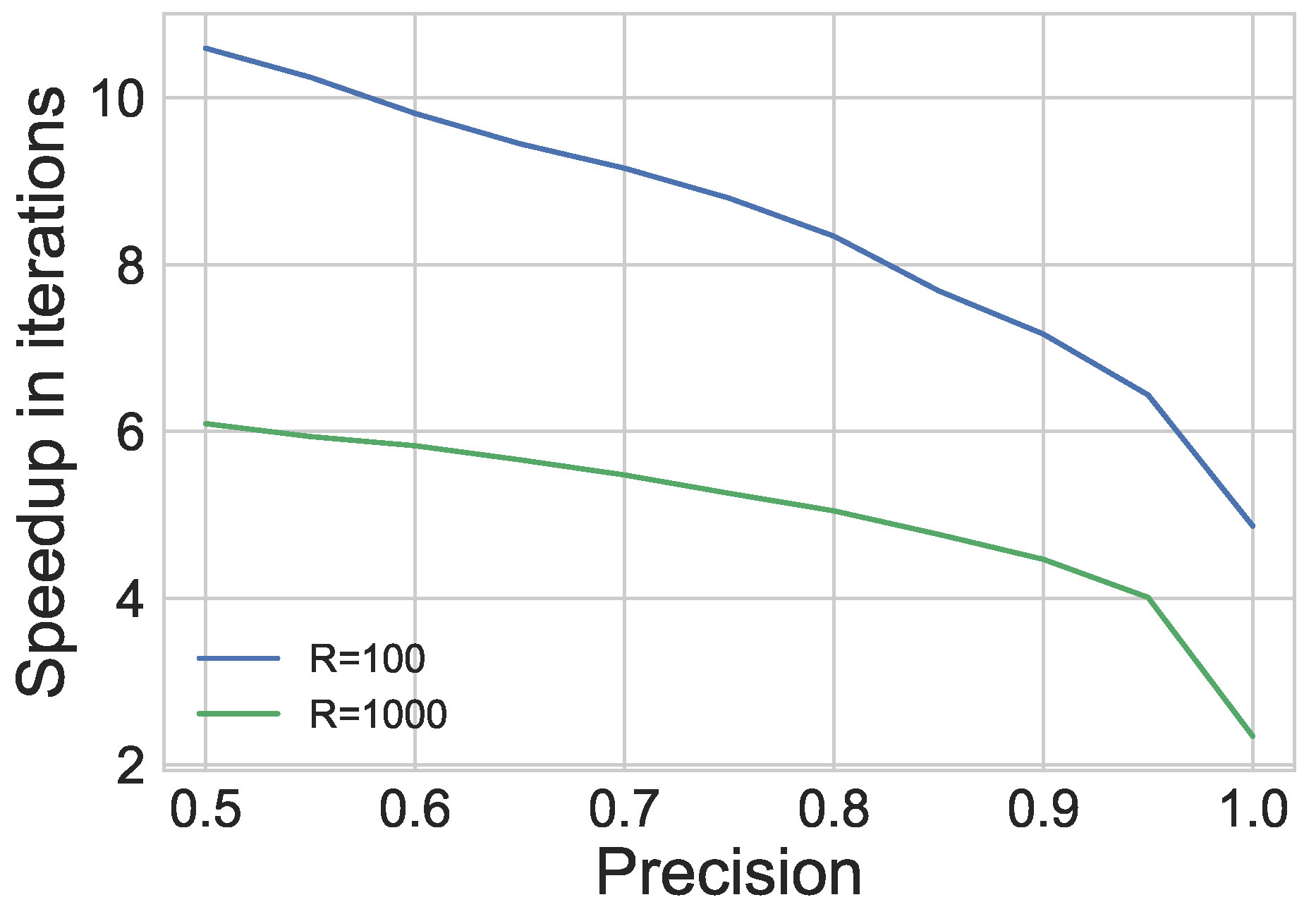
In previous sections to identify the top vertices in a graph, we have run the iterative solver to a predetermined tolerance to obtain an approximation of c P R * or c K a t z * . In this section, we introduce an alternate stopping criterion for an iterative solver that determines when to terminate based off of ranking accuracy of the highly ranked vertices instead of numerical accuracy of the solution using Theorem 1. If a user desires a set of the top R vertices, our stopping criterion returns a set of S vertices with at least some preset user-desired precision ϕ * . The precision for these values of R and S is defined as ϕ = R S 1 . We show in practice that this is faster than running a solver to machine precision, about 10 15 , which is the most precise numerical solution possible on a computer. Since our eventual goal is local community detection using the personalized centrality vector, we simply desire the set of the highly ranked vertices without concern for the internal ordering of the set, and we want only that the top R vertices are contained somewhere within the returned set of S vertices. Therefore, this new stopping criterion is particularly apt for this purpose.
We can implement this new stopping criterion as a part of the Jacobi iterative method. At each iteration of the iterative solver, the current solution c ( k ) is organized in decreasing order to produce the vector d ( k ) . To sort c ( k ) , we use the method described in Section 4.1. We find the first position S > R in d ( k ) where we have the necessary gap of | d R ( k ) d j ( k ) | > 2 ϵ k for whichever centrality metric we are currently calculating. If, for this value of S, we have at least the user-desired preset precision meaning ϕ > ϕ * , we terminate; otherwise, we iterate again to iteration k + 1 to obtain a more accurate approximation c ( k ) . Intuitively, the precision shows how far past position R we must travel down the vector to find the necessary gap to ensure we are returning the top R vertices in the graph.

6.2. Results

Since our stopping criterion is theoretically guaranteed to return the top R vertices with any user-desired precision ϕ * , we evaluate our method by comparing quality versus performance. Specifically, for different user-desired precisions, we calculate both (1) the raw number of iterations the solver takes to guarantee the set of top R as well as (2) the speedup obtained compared to iterating to machine precision for both PageRank and Katz.
We vary the precision ϕ * { 0 . 5 , 0 . 6 , 0 . 7 , 0 . 8 , 0 . 9 , 1 . 0 } and test values of R = 100 and 1000, or equivalently calculate communities of sizes 100 and 1000. For each graph and community size, we use five randomly chosen seeds to calculate the personalized centrality vector and results shown are averages over the five seeds. We use the same five datasets from Table 4.
Figure 4 plots the raw number of iterations taken for different values of the desired precision ϕ * for each graph for R = 100 (Figure 4a) and R = 1000 (Figure 4b) using personalized Katz centrality. We see that the number of iterations slowly increases up until a precision of ϕ * = 0 . 9 and then sharply increases for a perfect precision of ϕ * = 1 . 0 . The fact that the iteration count increases minimally for precisions of 0.5–0.9 shows our method can deliver fairly precise sets of top R vertices with minimal extra computation. Specifically, we can obtain fairly precise ( ϕ * = 0 . 9 ) sets of top R vertices (or in our case, local communities of size R) without much more work than, for example, a precision of ϕ * = 0 . 5 . It is only when we seek a precision of ϕ * = 1 . 0 that the iteration count sharply increases for all graphs, almost doubling in some cases. In many cases, the difference in iteration counts going from a precision of 0.9 to 1.0 is the same as the difference going from a precision of 0.5 to 0.9. Additionally, the overall number of iterations is much less for R = 100 compared to R = 1000 over all graphs and for both centrality metrics. This is because, regardless of the centrality metric, the gap ϵ k that we are looking for is fixed, while values in the centrality vector decrease exponentially. Thus, when we are looking for the gap ϵ k for larger values of R, we will need to traverse further down the ranking vector to obtain the necessary gap, and most probably require a more accurate numerical solution compared to the solution needed for smaller values of R.
The previous results have shown raw iteration counts for both centrality metrics for different values of R. Figure 5 therefore plots the speedup in iterations using our new stopping criterion compared to running the solver to machine precision. Denote the number of iterations taken by our method to obtain the top R vertices as I A and the number of iterations taken to run to machine precision as I M . We calculate speedup as I M I A . We plot speedup versus the user-desired precision for both R = 100 and R = 1000. Results are averaged over all the graphs tested. Similar to the results seen earlier, we see less speedup for R = 1000 compared to R = 100. Additionally, we obtain less speedup for more precise local communities returned. Intuitively, this again makes sense since we require a more accurate numerical solution for the more precise communities.
We have presented a method for discerning when the rank of vertex i above j is correct based on if there is a substantial gap between the centrality values of vertices i and j, respectively. However, it is quite possible to have vertex i with a score of 100 and vertex j with a score of 100.1, where ranking j higher than i would probably not change the result substantially. We therefore present a possible approach for handling group rankings rather than individual rankings, where the difference in value between two groups is substantial. Such a group ranking would not require precise sorting of the centrality vector; instead, some variation of bucket sort could be used where vertices are grouped in buckets based on a particular range of scores. This would be applicable in applications where the user has some a priori notion of the centrality values themselves and can set the ranges of scores accordingly. In situations such as community detection, group ranking can be more useful since the values of vertices themselves are not of utmost importance. The group ranking can function similarly to the method presented earlier for individual ranking. Rather than looking for gaps between vertices i and j, we can instead look for gaps between average values in the difference groups.
In this section, we presented a new stopping criterion for iterative solvers that allows us to theoretically guarantee when we have the top R vertices in a personalized centrality vector. We can then use this set as the local community, as we have explored in previous sections. All the results in this section have dealt with static graphs. The extension to dynamic graphs is quite straightforward: whenever the personalized centrality vector is updated using the dynamic algorithm for personalized Katz, the same theory in Theorem 1 can be applied to the updated centrality vector. We can then guarantee sets of top R vertices in dynamic graphs as well, which translate to the local communities in changing graph data. Future work will develop additional theory for guarantees for PageRank as well and will explore adapting the theory to update on the fly in dynamic graphs instead of having to recompute the bound from scratch every time the graph changes.

7. Conclusions

The problems of community detection and centrality have been well-studied in recent years. In this work, we have bridged these two fields by presenting a new method of identifying local communities using personalized centrality metrics.
We extended our previous work in [1,2,3] by using dynamic algorithms for calculating centrality scores in order to find local communities in evolving networks.
Our method uses the top R highly ranked vertices from a personalized centrality metric as the local community with respect to seed vertices of interest. Experiments on synthetic networks show that our method is able to identify blocks in artificially generated stochastic block models. We have shown that we obtain a high recall of the vertices using our method compared to the ground truth and that our method is faster than conventional local community detection methods such as greedy seed set expansion. Next, we extended our method to detect evolving communities in dynamic graphs. Using a synthetic example of a stochastic block model graph overlaid on an R-MAT background, we showed that our method successfully detects merging and splitting of communities over time. We applied our methods to real graphs and showed that our algorithm yields similar quality communities to static recomputation and is faster in both time and the number of iterations taken. Finally, we presented theory for guaranteeing the correct ordering of vertices from an approximation of a centrality vector to the exact solution. Since we are able to guarantee the highly ranked vertices as correct in an approximation, we know that the vertices returned in the local community are indeed the exact highly ranked vertices from the exact solution.
The main drawback of our method is that it requires previous knowledge of the community size. Future work will investigate methods to identify the local community using personalized centrality without previous knowledge of community size. For example, we can use a sweep cut method similar to [38]. After the personalized centrality metric is calculated using our dynamic algorithm, we can sweep over all cuts induced by the ordering of the personalized centrality vector and choose the best cut determined by conductance scores of the induced cuts. This method would therefore identify the best local community given the centrality scores without any size requirement. We also could combine the termination criteria with the gap between centrality values to maintain only a limited portion of the centrality vector. Future work will also extend the theory to dynamic graphs so we are able to ensure correctness of vertices returned in evolving networks over time instead of recomputing the theoretical guarantee each time the underlying graph changes. Since local communities with respect to a seed vertex can be computed independently of other local communities with respect to different seeds, the computation of separate communities can be easily parallelized. By computing multiple local communities across an entire graph, we can partition the global graph into different communities. This can also be addressed in future work.

Acknowledgments

The work depicted in this paper was partially sponsored by the Defense Advanced Research Projects Agency (DARPA) under agreement #HR0011-13-2-0001. The content, views and conclusions presented in this document do not necessarily reflect the position or the policy of DARPA or the U.S. Government, and no official endorsement should be inferred. Distribution Statement A: “Approved for public release; distribution is unlimited.” This work was also partially sponsored by NSF Grant ACI-1339745 (XScala). We thank Oracle for the hardware platform and reviewers for their careful attention to detail, relevant references, and useful suggestions.

Author Contributions

Eisha Nathan and Anita Zakrzewska constructed the experiments and wrote the majority of the paper. Jason Riedy wrote pieces of the paper and edited heavily. David A. Bader provided guidance and editing.

Conflicts of Interest

The authors declare no conflict of interest. The funding sponsors had no role in the design of the study; in the collection, analyses, or interpretation of data; in the writing of the manuscript, and in the decision to publish the results.

References

  1. Nathan, E.; Sanders, G.; Fairbanks, J.; Bader, D.A.; Henson, V.E. Graph Ranking Guarantees for Numerical Approximations to Katz Centrality. Procedia Comput. Sci. 2017, 108, 68–78. [Google Scholar] [CrossRef]
  2. Nathan, E.; Bader, D.A. A Dynamic Algorithm for Updating Katz Centrality in Graphs. In Proceedings of the 2017 IEEE/ACM International Conference on Advances in Social Networks Analysis and Mining, Sydney, Australia, 31 July–3 August 2017. [Google Scholar]
  3. Riedy, J. Updating PageRank for Streaming Graphs. In Proceedings of the 2016 IEEE International Parallel and Distributed Processing Symposium Workshops, Chicago, IL, USA, 23–27 May 2016; pp. 877–884. [Google Scholar]
  4. Chung, F.R. Spectral Graph Theory; American Mathematical Society: Providence, RI, USA, 1997; Volume 92. [Google Scholar]
  5. Havemann, F.; Heinz, M.; Struck, A.; Gläser, J. Identification of overlapping communities and their hierarchy by locally calculating community-changing resolution levels. J. Stat. Mech. Theory Exp. 2011. [Google Scholar] [CrossRef]
  6. Newman, M.E.; Girvan, M. Finding and evaluating community structure in networks. Phys. Rev. E 2004, 69, 026113. [Google Scholar] [CrossRef] [PubMed]
  7. Bader, D.A.; Meyerhenke, H.; Sanders, P.; Wagner, D. Graph partitioning and graph clustering. In Contemporary Mathematics, Proceedings of the 10th DIMACS Implementation Challenge Workshop, Atlanta, GA, USA, 13–14 February 2012; American Mathematical Society: Providence, RI, USA, 2013; Volume 588. [Google Scholar]
  8. Katz, L. A new status index derived from sociometric analysis. Psychometrika 1953, 18, 39–43. [Google Scholar] [CrossRef]
  9. Benzi, M.; Klymko, C. A matrix analysis of different centrality measures. arXiv 2014, arXiv:1312.6722. [Google Scholar]
  10. Page, L.; Brin, S.; Motwani, R.; Winograd, T. The PageRank Citation Ranking: Bringing Order to the Web; Technical Report 1999-66; Stanford InfoLab: Stanford, CA, USA, 1999. [Google Scholar]
  11. Brandes, U.; Pich, C. Centrality estimation in large networks. Int. J. Bifurc. Chaos 2007, 17, 2303–2318. [Google Scholar] [CrossRef]
  12. Saad, Y. Iterative Methods for Sparse Linear Systems; SIAM: Philadelphia, PA, USA, 2003. [Google Scholar]
  13. Clauset, A.; Newman, M.E.; Moore, C. Finding community structure in very large networks. Phys. Rev. E 2004, 70, 066111. [Google Scholar] [CrossRef] [PubMed]
  14. Blondel, V.D.; Guillaume, J.L.; Lambiotte, R.; Lefebvre, E. Fast unfolding of communities in large networks. J. Stat. Mech. Theory Exp. 2008. [Google Scholar] [CrossRef]
  15. Pothen, A.; Simon, H.D.; Liou, K.P. Partitioning sparse matrices with eigenvectors of graphs. SIAM J. Matrix Anal. Appl. 1990, 11, 430–452. [Google Scholar] [CrossRef]
  16. Derényi, I.; Palla, G.; Vicsek, T. Clique percolation in random networks. Phys. Rev. Lett. 2005, 94, 160202. [Google Scholar] [CrossRef] [PubMed]
  17. Xie, J.; Szymanski, B.K.; Liu, X. SLPA: Uncovering overlapping communities in social networks via a speaker-listener interaction dynamic process. In Proceedings of the 2011 IEEE 11th International Conference on Data Mining Workshops (ICDMW), Vancouver, BC, Canada, 11 December 2011; pp. 344–349. [Google Scholar]
  18. Xie, J.; Szymanski, B.K. Towards linear time overlapping community detection in social networks. In Advances in Knowledge Discovery and Data Mining; Springer: Berlin, Germany, 2012; pp. 25–36. [Google Scholar]
  19. Evans, T.; Lambiotte, R. Line graphs of weighted networks for overlapping communities. Eur. Phys. J. B 2010, 77, 265–272. [Google Scholar] [CrossRef]
  20. Lancichinetti, A.; Radicchi, F.; Ramasco, J.J.; Fortunato, S. Finding statistically significant communities in networks. PLoS ONE 2011, 6, e18961. [Google Scholar] [CrossRef] [PubMed]
  21. Lancichinetti, A.; Fortunato, S.; Kertész, J. Detecting the overlapping and hierarchical community structure in complex networks. New J. Phys. 2009, 11, 033015. [Google Scholar] [CrossRef]
  22. Lee, C.; Reid, F.; McDaid, A.; Hurley, N. Detecting highly overlapping community structure by greedy clique expansion. In Proceedings of the 4th SNA-KDD Workshop, Washington, DC, USA, 25–28 July 2010; pp. 33–42. [Google Scholar]
  23. Staudt, C.L.; Meyerhenke, H. Engineering Parallel Algorithms for Community Detection in Massive Networks. IEEE Trans. Parallel Distrib. Syst. 2016, 27, 171–184. [Google Scholar] [CrossRef]
  24. Tantipathananandh, C.; Berger-Wolf, T.; Kempe, D. A framework for community identification in dynamic social networks. In Proceedings of the 13th ACM SIGKDD International Conference on Knowledge Discovery and Data Mining, San Jose, CA, USA, 12–15 August 2007; pp. 717–726. [Google Scholar]
  25. Mucha, P.J.; Richardson, T.; Macon, K.; Porter, M.A.; Onnela, J.P. Community structure in time-dependent, multiscale, and multiplex networks. Science 2010, 328, 876–878. [Google Scholar] [CrossRef] [PubMed]
  26. Jdidia, M.B.; Robardet, C.; Fleury, E. Communities detection and analysis of their dynamics in collaborative networks. In Proceedings of the 2nd International Conference on Digital Information Management, Lyon, France, 28–31 October 2007; pp. 744–749. [Google Scholar]
  27. Chakrabarti, D.; Kumar, R.; Tomkins, A. Evolutionary clustering. In Proceedings of the 12th ACM SIGKDD International Conference on Knowledge Discovery and Data Mining, Philadelphia, PA, USA, 20–23 August 2006; pp. 554–560. [Google Scholar]
  28. Lin, Y.R.; Chi, Y.; Zhu, S.; Sundaram, H.; Tseng, B.L. Analyzing communities and their evolutions in dynamic social networks. ACM Trans. Knowl. Discov. Data 2009, 3, 8. [Google Scholar] [CrossRef]
  29. Aynaud, T.; Guillaume, J.L. Static community detection algorithms for evolving networks. In Proceedings of the WiOpt’10: Modeling and Optimization in Mobile, Ad Hoc, and Wireless Networks, Avignon, France, 31 May–4 June 2010; pp. 508–514. [Google Scholar]
  30. Shang, J.; Liu, L.; Xie, F.; Chen, Z.; Miao, J.; Fang, X.; Wu, C. A real-time detecting algorithm for tracking community structure of dynamic networks. arXiv 2014, arXiv:1407.2683. [Google Scholar]
  31. Dinh, T.N.; Xuan, Y.; Thai, M.T. Towards social-aware routing in dynamic communication networks. In Proceedings of the 2009 IEEE 28th International Performance Computing and Communications Conference (IPCCC), Scottsdale, AZ, USA, 14–16 December 2009; pp. 161–168. [Google Scholar]
  32. Riedy, J.; Bader, D.A. Multithreaded community monitoring for massive streaming graph data. In Proceedings of the 2013 IEEE 27th International Symposium on Parallel and Distributed Processing Workshops and PhD Forum IEEE, Boston, MA, USA, 20–24 May 2013; pp. 1646–1655. [Google Scholar]
  33. Görke, R.; Maillard, P.; Schumm, A.; Staudt, C.; Wagner, D. Dynamic graph clustering combining modularity and smoothness. ACM J. Exp. Algorithmics 2013, 18, 1–5. [Google Scholar] [CrossRef]
  34. Clauset, A. Finding local community structure in networks. Phys. Rev. E 2005, 72, 026132. [Google Scholar] [CrossRef] [PubMed]
  35. Freeman, L.C. A set of measures of centrality based on betweenness. Sociometry 1977, 40, 35–41. [Google Scholar] [CrossRef]
  36. Girvan, M.; Newman, M.E. Community structure in social and biological networks. Proc. Natl. Acad. Sci. USA 2002, 99, 7821–7826. [Google Scholar] [CrossRef] [PubMed]
  37. Bagrow, J.P.; Bollt, E.M. Local method for detecting communities. Phys. Rev. E 2005, 72, 046108. [Google Scholar] [CrossRef] [PubMed]
  38. Andersen, R.; Chung, F.; Lang, K. Local graph partitioning using PageRank vectors. In Proceedings of the 47th Annual IEEE Symposium on Foundations of Computer Science, Berkeley, CA, USA, 21–24 October 2006; pp. 475–486. [Google Scholar]
  39. Chen, Y.Y.; Gan, Q.; Suel, T. Local methods for estimating PageRank values. In Proceedings of the thirteenth ACM International Conference on Information and Knowledge Management, Washington, DC, USA, 8–13 November 2004; pp. 381–389. [Google Scholar]
  40. Chien, S.; Dwork, C.; Kumar, R.; Sivakumar, D. Towards exploiting link evolution. In Proceedings of the Workshop on Algorithms and Models for the Web Graph; 2001. Available online: http://citeseerx.ist.psu.edu/viewdoc/summary?doi=10.1.1.16.811 (accessed on 29 August 2017).
  41. Sarma, A.D.; Gollapudi, S.; Panigrahy, R. Estimating PageRank on graph streams. J. ACM 2011, 58, 13. [Google Scholar] [CrossRef]
  42. Gyöngyi, Z.; Garcia-Molina, H.; Pedersen, J. Combating web spam with trustrank. In Proceedings of the Thirtieth International Conference on Very Large Data Bases—Volume 30, Toronto, ON, Canada, 31 August–3 September 2004; pp. 576–587. [Google Scholar]
  43. Langville, A.N.; Meyer, C.D. Updating PageRank Using the Group Inverse and Stochastic Complementation; Technical Report CRSC-TR02-32; North Carolina State University: Raleigh, NC, USA, 2002. [Google Scholar]
  44. Langville, A.N.; Meyer, C.D. Updating the stationary vector of an irreducible Markov chain with an eye on Google’s PageRank. SIAM. J. Matrix Anal. Appl. 2004, 27, 968–987. [Google Scholar] [CrossRef]
  45. Langville, A.N.; Meyer, C.D. Updating PageRank with iterative aggregation. In Proceedings of the 13th International World Wide Web conference on Alternate Track Papers & Posters, New York, NY, USA, 17–22 May 2004; pp. 392–393. [Google Scholar]
  46. Bahmani, B.; Chowdhury, A.; Goel, A. Fast incremental and personalized PageRank. Proc. VLDB Endow. 2010, 4, 173–184. [Google Scholar] [CrossRef]
  47. Arrigo, F.; Grindrod, P.; Higham, D.J.; Noferini, V. Nonbacktracking Walk Centrality for Directed Networks; Technical Report MIMS Preprint 2017.9; University of Manchester: Manchester, UK, 2017. [Google Scholar]
  48. Leskovec, J.; Lang, K.J.; Dasgupta, A.; Mahoney, M.W. Statistical properties of community structure in large social and information networks. In Proceedings of the 17th International Conference on World Wide Web, Beijing, China, 21–25 April 2008; pp. 695–704. [Google Scholar]
  49. Kloumann, I.M.; Ugander, J.; Kleinberg, J.M. Block Models and Personalized PageRank. Proc. Natl. Acad. Sci. USA 2016, 114, 33–38. [Google Scholar] [CrossRef] [PubMed]
  50. Moler, C.B. Iterative Refinement in Floating Point. J. ACM 1967, 14, 316–321. [Google Scholar] [CrossRef]
  51. Chakrabarti, D.; Zhan, Y.; Faloutsos, C. R-MAT: A Recursive Model for Graph Mining. In Proceedings of the Fourth SIAM International Conference on Data Mining, Lake Buena Vista, FL, USA, 22–24 April 2004; pp. 442–446. [Google Scholar]
  52. Kunegis, J. KONECT: the Koblenz network collection. In Proceedings of the 22nd International Conference on World Wide Web, Rio de Janeiro, Brazil, 13–17 May 2013; pp. 1343–1350. [Google Scholar]
  53. Riedy, J.; Bader, D.A.; Jiang, K.; Pande, P.; Sharma, R. Detecting Communities from Given Seeds in Social Networks; Technical Report; Georgia Institute of Technology: Atlanta, GA, USA, 2011. [Google Scholar]
Figure 1. The speedup of the personalized Katz centrality method compared to greedy expansion is shown for SBM graphs with different parameters. (a) The number of vertices n in the graph varies, with d = 20 and k = 2 . (b) The number of communities k in the graph varies, with n = 47104 and d = 20 . (c) The average vertex degree d varies, with n = 1000 and k = 2 .
Algorithms 10 00102 g001aAlgorithms 10 00102 g001b
Figure 2. Synthetic dynamic graph showing merging and splitting of communities. (a) t = 1 , (b) t = 2 , (c) t = 3 , (d) t = 4 .
Algorithms 10 00102 g002
Figure 3. Performance and quality behavior of dynamic algorithm compared to static recomputation over time. (a) speedup in iterations over time for b = 10, (b) ratio of conductance scores over time for b = 100.
Algorithms 10 00102 g003
Figure 4. Katz precision vs. iteration count. (a) R = 100, (b) R = 1000.
Algorithms 10 00102 g004
Figure 5. Speedup in iterations.
Algorithms 10 00102 g005
Table 1. Contributions and main results presented in this paper.
ContributionMain Results
New method of identifying local communities using personalized centrality metrics• Comparisons to a modified version of greedy seed set expansion4
• High recall values comparing our method to ground truth on stochastic block model graphs
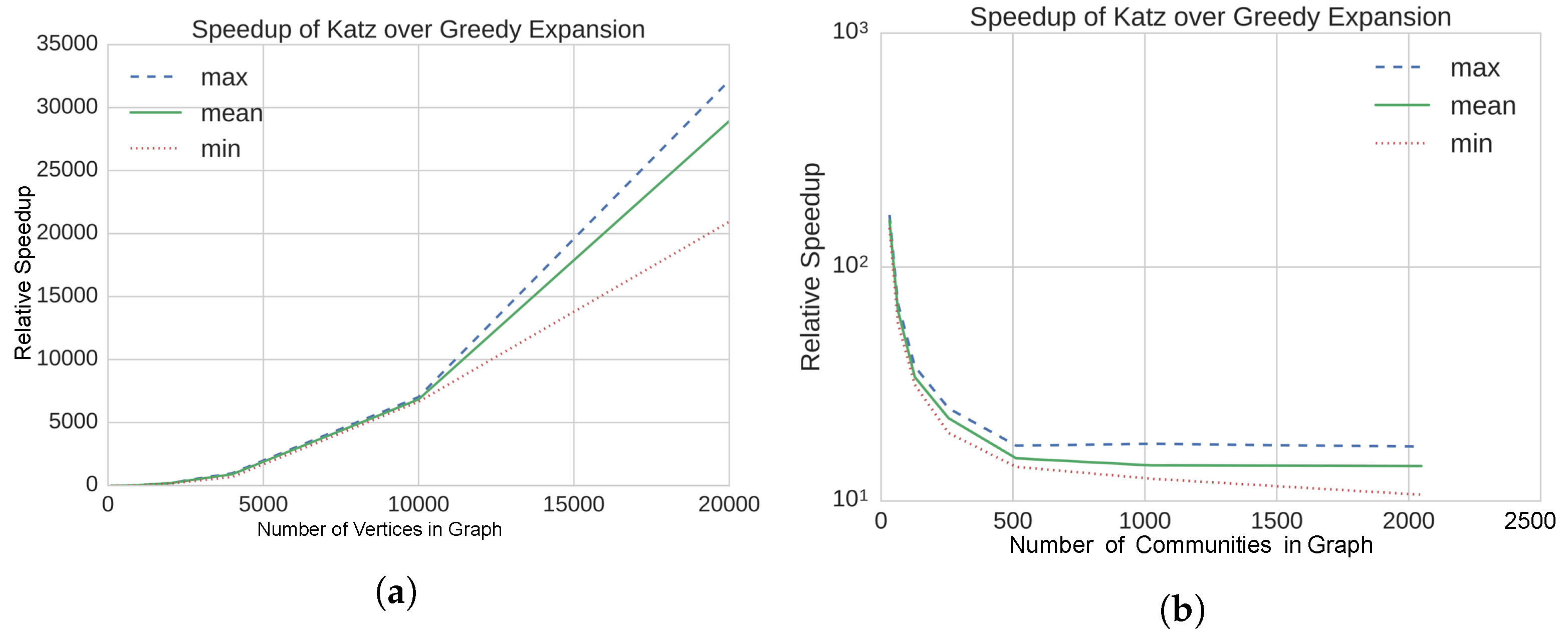
• Several orders of magnitude of speedup obtained using our method
Dynamic algorithm to identify local communities in evolving networks• Recalls of over 0.80 for synthetic networks showing community evolution5
• Speedups of over 60× execution time improvement compared to static recomputation for real graphs
• Good quality of communities returned by our dynamic method w.r.t. ratios of conductance and normalized edge cut
• Quality of communities is preserved over time for real graphs
• Comparisons using multiple seeds for our algorithm show our method is robust to using many seeds
Numerical theory to guarantee the accuracy of an approximate solution to a centrality metric• Development of a new stopping criterion for iterative solvers to terminate when we can guarantee rankings given desired precision6
• Speedups obtained compared to running to preset tolerance versus using our new stopping criterion
Table 2. The quality of communities detected with our personalized Katz method and greedy expansion is shown. Test graphs are stochastic block model (SBM) graphs with n = 1000 and k = 2 . (a) The average vertex degree d is varied, while ρ = 0 . 01 . (b) The proportion of inter-community edges ρ is varied, while d = 20 . (c) The proportion of inter-community edges ρ is varied, while d = 100 .
(a)
Avg. Degree ρ Katz RecallGreedy RecallForced Greedy Recall
MinMeanMaxMinMeanMaxMinMeanMax
50.010.6880.9360.9740.0040.0150.0340.0240.9241.000
100.010.9200.9880.9980.0020.1041.0000.0020.9701.000
200.010.9740.9971.0000.0020.9021.0000.0020.9901.000
500.010.9940.9991.0000.0020.9901.0000.0020.9901.000
1000.010.9900.9981.0000.0020.9901.0000.0020.9901.000
2500.011.0001.0001.0000.0020.9901.0000.0020.9901.000
4900.011.0001.0001.0000.0020.9901.0000.0020.9901.000
(b)
Avg. Degree ρ Katz RecallGreedy RecallForced Greedy Recall
MinMeanMaxMinMeanMaxMinMeanMax
200.010.9740.9971.0000.0020.9021.0000.0020.9901.000
200.050.8060.9440.9880.0020.8521.0000.0020.9601.000
200.10.6780.8330.9100.0020.7731.0000.0020.8691.000
200.20.5020.6380.7300.0020.6030.9980.0080.8330.998
200.30.4740.5510.6300.0020.5050.9320.0960.6550.942
200.40.4560.5080.5420.0060.3540.5940.4160.5210.604
(c)
Avg. Degree ρ Katz RecallGreedy RecallForced Greedy Recall
MinMeanMaxMinMeanMaxMinMeanMax
1000.010.9900.9981.0000.0020.9901.0000.0020.9901.000
1000.050.9800.9901.0000.0020.9601.0000.0020.9601.000
1000.10.9420.9800.9920.0020.9401.0000.0020.9401.000
1000.20.7280.8220.9080.0020.8801.0000.0020.8801.000
1000.30.5520.6260.7000.0020.8281.0000.0020.8281.000
1000.40.4820.5300.5760.0700.6040.9360.0740.6120.944
Table 3. Average recalls at each point in time for synthetic merging and splitting of communities over time.
Block Size = 100Block Size = 1000
ParametersBatch Sizet =12341234
R =1002002001001000200020001000
p i n = 0.2,
p o u t = 0.01
10 0.860.940.930.850.930.970.989.98
100 0.760.890.890.750.970.990.990.97
1000 0.760.840.840.660.930.970.970.93
p i n = 0.5,
p o u t = 0.01
10 0.920.960.970.920.960.980.990.99
100 0.790.890.900.780.950.980.980.95
1000 0.880.910.910.820.960.990.990.96
Average0.830.910.910.800.950.980.980.96
Table 4. Real graphs used in experiments. Columns are graph name, number of vertices, and number of edges.
Graph | V | | E |
slashdot-threads51,083140,778
enron87,2211,148,072
digg279,6301,731,653
wiki-talk541,3552,424,962
youtube-u-growth3,223,5899,375,374
Table 5. Average summary statistics over time on real graphs for all batch sizes. Columns are graph name, batch size, speedup in time, speedup in iterations, recall, ratio of conductance scores, and ratio of normalized edge cut scores.
GraphBatch SizePerformanceQuality
T S / T D I S / I D Recall ϕ S / ϕ D f S / f D
slashdot-threads1052.94×34.02×0.930.991.03
10026.88×21.46×0.961.001.01
100039.65×31.09×0.961.001.00
enron1075.42×45.04×0.971.001.00
10063.61×41.28×0.981.010.98
100046.20×29.57×0.961.010.98
digg1054.29×29.41×0.860.971.18
10047.64×25.69×0.900.981.07
100050.64×26.87×0.970.991.02
wiki-talk1056.02×36.68×0.951.001.02
10048.87×31.46×0.910.991.19
100056.22×36.95×0.961.001.02
youtube- u-growth1056.47×27.66×0.961.000.94
10050.00×26.58×0.961.001.00
100040.17×20.44×0.911.000.92
Table 6. Results for different seeding methods. Columns are graph name, seeding method, speedup in time, speedup in iterations, recall, ratio of conductance scores, and ratio of normalized edge cut scores. Results shown are averaged over all graphs.
GraphMethodNumber of Seeds
12345678910
T S / T D RW-146.9×54.4×49.3×41.7×39.4×30.3×32.4×47.3×41.5×29.3×
RW-233.7×66.1×42.8×51.5×57.0×52.1×50.6×46.1×53.2×39.0×
RW-344.5×53.4×54.0×44.3×53.6×44.5×53.0×63.2×68.5×47.8×
I S / I D RW-129.4×30.9×29.8×24.6×24.5×24.4×21.0×29.2×25.3×22.3×
RW-220.4×37.3×24.4×30.9×31.8×29.2×29.0×28.4×30.1×24.1×
RW-326.0×29.8×31.9×27.9×33.4×27.4×30.9×38.2×37.0×29.9×
RecallRW-10.990.981.000.981.001.000.990.981.001.00
RW-20.960.980.950.990.960.991.000.990.990.99
RW-30.930.970.950.990.980.990.990.980.990.99
ϕ S / ϕ D RW-11.001.001.001.001.001.001.001.001.001.00
RW-21.001.001.001.001.001.001.001.001.001.00
RW-31.001.001.001.001.001.001.001.001.001.00
f S / f D RW-10.990.981.001.001.001.000.941.010.981.00
RW-21.000.970.991.011.031.001.001.001.001.00
RW-31.030.991.011.001.001.001.001.001.001.01

