Dependent Shrink of Transitions for Calculating Firing Frequencies in Signaling Pathway Petri Net Model

Abstract

Despite the recent rapid progress in high throughput measurements of biological data, it is still difficult to gather all of the reaction speed data in biological pathways. This paper presents a Petri net-based algorithm that can derive estimated values for non-valid reaction speeds in a signaling pathway from biologically-valid data. In fact, these reaction speeds are reflected based on the delay times in the timed Petri net model of the signaling pathway. We introduce the concept of a “dependency relation” over a transition set of a Petri net and derive the properties of the dependency relation through a structural analysis. Based on the theoretical results, the proposed algorithm can efficiently shrink the transitions with two elementary structures into a single transition repeatedly to reduce the Petri net size in order to eventually discover all transition sets with a dependency relation. Finally, to show the usefulness of our algorithm, we apply our algorithm to the IL-3 Petri net model.

1. Introduction

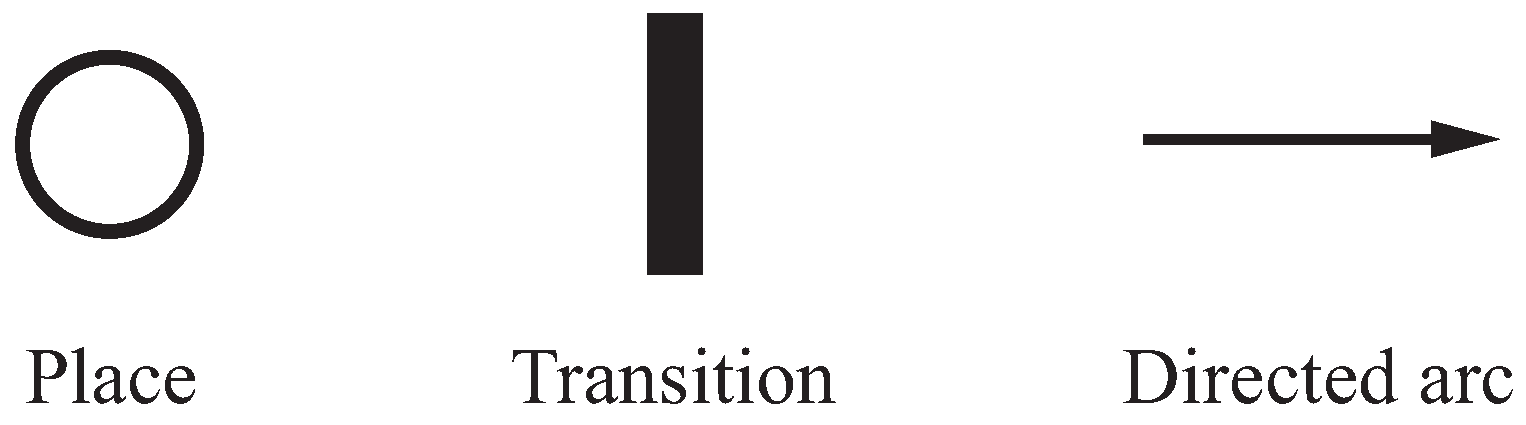
A Petri net [1,2] is a solid mathematical representation used in concurrent systems modeling, enabling a formal and clear representation of biological pathways at different time and scale levels [3]. Structurally, a Petri net is a directed bipartite graph, including two types of nodes, places and transitions and tokens contained in places. A state of a Petri net is expressed by a token distribution over the places and can be changed by the firing of transitions. The first Petri net model of a biological pathway [4] is a metabolic pathway, describing the conversion of metabolites through enzyme-catalyzed chemical reactions, which has been extensively studied regarding the structural [5,6,7,8] and dynamic [9,10,11] properties.

A signaling pathway is another major biological pathway, consisting of cascades of activated/deactivated proteins or protein complexes, through which signals are propagated from the cell surface to the nucleus. A Petri net has been used as a structural modeling framework for a signal pathway in a knowledge representation [12] and for data implementation in a database [13].

Modularization of a Petri net model into biologically-functional parts in a signaling pathway has been demonstrated using the fundamental behavioral property, T-invariant [14], which was formalized in metabolic pathways before [5,6,7,8], and its extended property, the feasible T-invariant [15]. Here, a T-invariant is a firing counting vector of transitions in a periodic firing sequence that leads back to the original token distribution where it starts from. A technique to automatically classify T-invariants into functional modules in a biological pathway was proposed in [16] based on cluster analysis. Another classification of T-invariants in terms of biological network structure was demonstrated in [17], where hierarchically-structured Petri net representations are derived automatically. T-invariant was further applied for the representation of the enzymatic activation process in a signaling pathway [18]. The dynamic behaviors of a signaling pathway were examined in Petri net models for a token amount, reflecting the concentration levels of molecules obtained based on the order of the transition firings specified by the topological motifs in a signaling pathway [19,20], and were calculated after reducing the number of parameters through a simplification process of a Petri net model [21].

The experimentally uncovered biological facts are usually summarized in a picture of a network structured by figures of various shapes and several type of arrows reflecting biological images. A Petri net allows us to model a biological pathway with maintaining its structural information, owing to the characteristics of the graphical representation of Petri net. Accordingly, Petri net-based modeling does not produce a negative effect of the abstraction in a modeling process compared to other modeling methods, such as differential equation-based methods.

The timed Petri net is a type of Petri net, in which time delay is associated with state transition, and is a promising candidate for modeling the dynamic property of a signaling pathway because the delay time of a transition is able to reflect the rate of a corresponding reaction in a signaling pathway. However, in the works above [18,19,20,21], a timed Petri net has not been employed.

The first attempt to use a timed Petri net for the modeling of a signaling pathway was in [22] (the “time” Petri net, which has a different extension in terms of time to the “timed” Petri net, was applied to model metabolic pathways in [11]), where the delay times were calculated based on a simple rule in which the sum of the consumption is equal to the production, so as to maintain the concentration equilibrium for each substance in a signaling pathway. Such Petri nets satisfying this simple rule are called retention-free Petri nets later and introduced as a new concept enabling a more flexible determination of the delay times using a concrete algorithm [23]. Cycles and inhibitory arcs, which often appear in signaling pathways, are treated in [24], but have not been incorporated owing to the difficulties in their structural handling.

These works [22,23,24] have studied a Petri net-based methodology to calculate estimated values for non-valid reaction speeds from a valid reaction speed, namely a biologically-measured speed, in the signaling pathway. A simple question therefore arises. How many and which reactions should be biologically measured in order to obtain all of the delay times in a Petri net model through the proposed methodology? This paper answers this question by introducing the concept of a “dependency relation” over a transition set of a Petri net, by which the transition set is divided into equivalence classes in the sense of a dependency relation, namely an equivalence relation. In fact, the number of equivalence classes is the number of reactions that should be biologically measured.

One possible way to find such an equivalence class is to establish a series of linear equations for all places based on the retention-freeness, solve the simultaneous equations to obtain the dependent solutions and, finally, determine the transitions with a dependency relation. However, this will take plenty of computation time for a given large-scale signaling pathway model. To cope with this problem, this paper gives an efficient algorithm to reduce the size of a Petri net through a structural analysis and, finally, to discover these equivalence classes.

The remainder of this paper is organized as follows. Section 2 provides the necessary definitions of Petri nets, and Section 3 introduces a timed Petri net and retention-free Petri net ($RFPN$). In Section 4, the concept of a dependency relation over the transitions of $RFPN$ is introduced, and related properties are derived through a structural analysis. In Section 5, based on the theoretical results of Section 4, an algorithm is proposed and applied to the IL-3 Petri net model to show its usefulness. Finally, Section 6 provides some concluding remarks and describes some future works.

2. Basic Definitions and Modeling Rules

In this section, we briefly provide the necessary definitions of a Petri net. For detailed descriptions, the reader is suggested to refer to [2].

Definition 1.

A Petri net (or a net for short), denoted by $PN=(T,P,E,\alpha ,\beta )$, is a bipartite graph consisting of elements shown in Figure 1, where:

• T is a set of transitions {$t_1,t_2,\cdots ,t_{\left|T\right|}$};
• P is a set of places {$p_1,p_2,\cdots ,p_{\left|P\right|}$};
• $E=E^{+}\cup E^{-}$, and $E^{+}$ and $E^{-}$ are respectively the sets of arcs from transitions to places $e=(t,p)$ and from places to transitions $e=(p,t)$;
• ${\alpha }_e$ is the weight of the arc expressed by positive integer $e=(p,t)$; and
• ${\beta }_e$ is the weight of the arc expressed by positive integer $e=(t,p)$.

Definition 2.

Let $PN=(T,P,E,\alpha ,\beta )$ be a Petri net.

• ${}^{•}t$ ($t^{•}$) is the set of input (output) places of $t\in T$, and ${}^{•}p$ ($p^{•}$) is the set of input (output) transitions of $p\in P$.
• A transition without an input arc is called the source transition, and the set of source transitions is denoted by $T_{src}=\{t_1^{src},\cdots ,t_a^{src}\}(a\ge 1).$
• A transition without an output arc is called the sink transition, and the set of sink transitions is denoted by $T_{sink}=\{t_1^{sink},\cdots ,t_b^{sink}\}(b\ge 1).$
• A transition t is called the synchronous transition if there exists a set of input places $P_s$ that for any $p\in P_s$, $p^{•}=\left\{t\right\}$ holds, and is defined by $T_{sync}=\{t_1^{sync},\cdots ,t_c^{sync}\}(c\ge 1)$.
• A place can hold a positive integer that represents a number of tokens. An assignment of tokens in places expressed in the form of a vector M is called a marking, which varies during the execution of a Petri net. Given an initial marking $M_0$, a Petri net is called a marked Petri net and is denoted by $MPN=(PN,M_o)$.

Figure 2 shows the source (i) and sink (ii) transitions, and Figure 3 shows a synchronous transition. Note that we use discrete Petri nets in the present study.

Definition 3.

A transition t is fireable if each input place $p_I$ of $PN$ has at least ${\alpha }_e$ tokens, where ${\alpha }_e$ denotes the weight of an arc $e=(p_I,t)$. The firing of a transition t removes ${\alpha }_e$ tokens from each input place $p_I$ of t and deposits ${\beta }_e(e=(t,p_O))$ tokens to each output place $p_O$ of t, where ${\beta }_e$ denotes the weight of an arc $e=(t,p_O)$. A source transition is always fireable.

Li et al. [18] gave the following modeling rules for signaling pathways based on a Petri net representation.

• Places denote static elements, including chemical compounds, conditions, states, substances and cellular organelles participating in the biological pathways. Tokens indicate the presence of such elements. The number of tokens can be regarded as a representation of the amount of chemical substances. The current assignment of tokens to the different places is expressed in the form of a vector, namely a marking, as defined above.
• Transitions denote active elements, including chemical reactions, events, actions, conversions and catalyzed reactions. A transition fires by taking off tokens from their individual input places and creating new tokens that are distributed to the output places if the input places have at least as many tokens in them as the arc weight from the place to the transition.
• Directed arcs connecting places and transitions represent the relations between corresponding static elements and active elements. Arc weights α and β (defined in Definition 1) describe the quantities of substances required before and after a reaction, respectively. Particularly in the case of modeling a chemical reaction, arc weights represent quantities given by stoichiometric equations of the reaction itself. Note that the weight of an arc is omitted if the weight is one.
• Because an enzyme itself acts as a catalyzer in biological pathways, and no consumption occurs in the biochemical reactions, an enzyme is exceptionally modeled in the following definition.
• An inhibition function in biological pathways is modeled by an inhibitor arc.

Definition 4.

An enzyme in a biological pathway is modeled by a place, called an enzyme place, as shown in Figure 4 [18].

• Enzyme place $p_i$ has a self-loop with the same weight connected from and to transition $t_s$. Once an enzyme place is occupied by a token, the token will return to the place again to maintain the fireable state if the transition $t_s$ is fired.
• Let $t_p$ and $t_d$ denote a token provider of $p_i$ and a sink output transition of $p_i$, respectively, where the firing of $t_p$ represents an enzyme activation reaction, and the firing of $t_d$ implies a small natural degradation in a biological pathway. $p_i$ holds up token(s) after firing transition $t_p$, and the weights of the arcs satisfy $\alpha (p_i,t_d)\ll \alpha (p_i,t_s)$.

3. Timed Petri Net and Retention-Free Petri Net

Petri nets are extended by assigning a delay time of the firing to each transition to facilitate a system-level understanding through means of a simulation. Such an extended Petri net is called a timed Petri net.

Definition 5.

Timed Petri net $TPN$ is defined by $TPN=(PN,D)$, where D is a set of positive numbers expressing the firing delay times (or delay time for short) of transitions in T. The firing rule of a $TPN$ is as follows:

• initially, all of the tokens are in a non-reserved state; once a transition $t_i$ is decided to have fired, the tokens required for firing are changed from the non-reserved state to the reserved state;
• when the delay time $d_i$ of $t_i$ has passed, $t_i$ fires to remove the reserved tokens from the input places of $t_i$ and put non-reserved tokens into the output places of $t_i$.

In a timed Petri net, the firing times of a transition $t_i$ per unit of time are called firing frequency $f_i$. $\overline{f_i}$ represents the maximum firing frequency of $t_i$. The delay time $d_i$ of $t_i$ is given by the reciprocal of $\overline{f_i}$.

Note that firing frequencies indicate reaction speed data in a biological pathway.

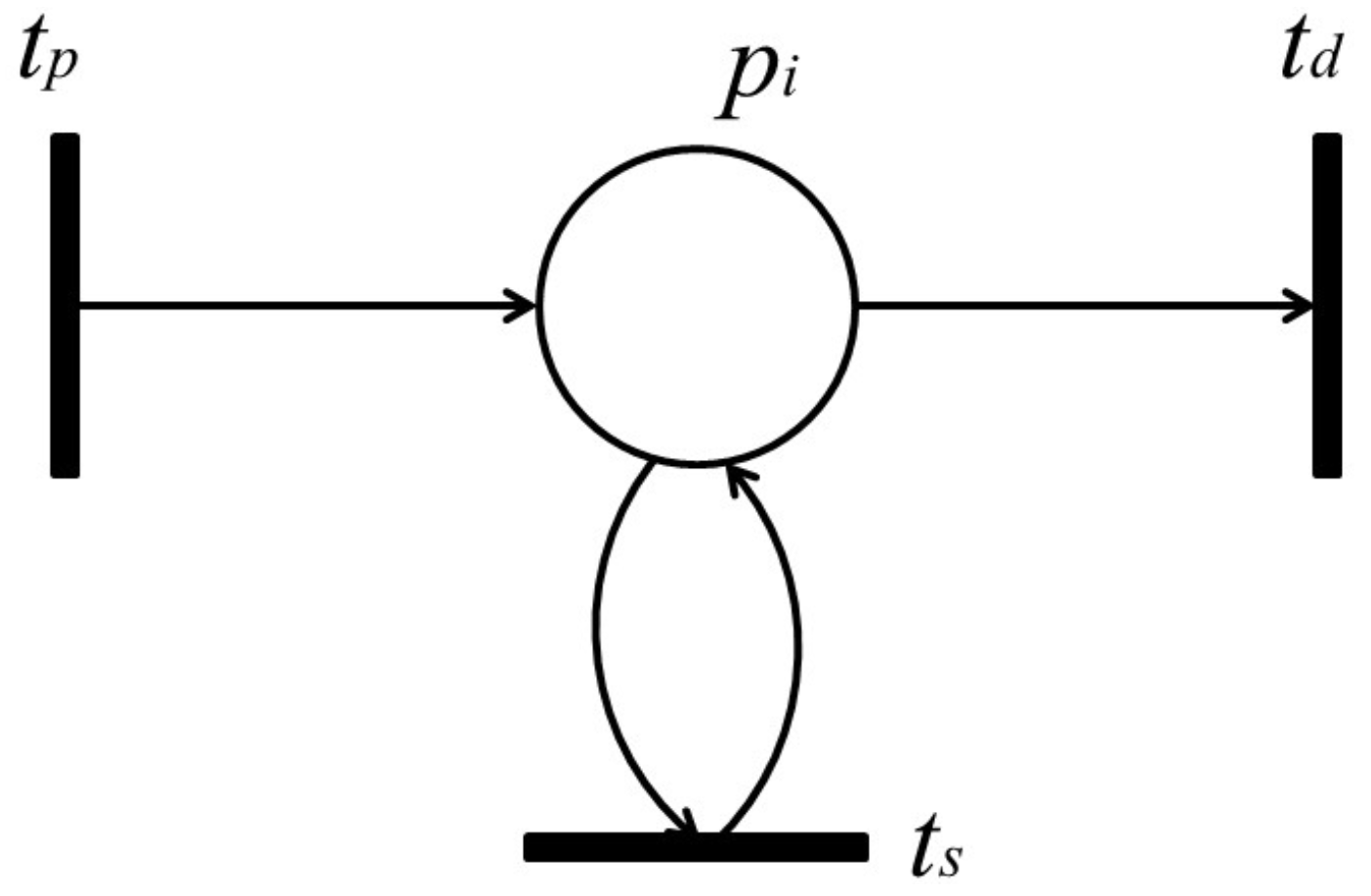
We show here the method of conflict resolution using stochastic decision rules. To resolve the conflict firing problem, there are three methods that can be adopted: priority, probabilistic choice and alternate firing [25]. The proposed firing rule given in this paper is to combine a probabilistic choice and alternate firing. We introduce a stochastic approach to determine the firings for a series of transitions in conflict (Figure 5), as defined in the following definition.

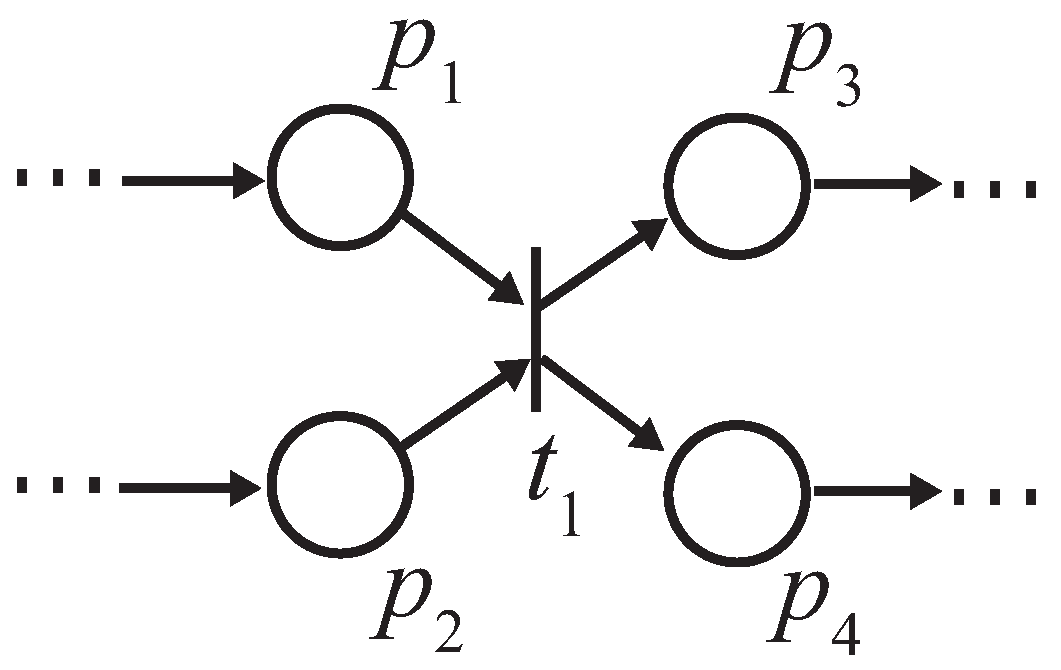
Definition 6.

Suppose a place p possesses output transitions, $t_{O_1},t_{O_2},\cdots ,t_{O_n}$, as shown in Figure 5. Then, the firing rule is as follows [23]:

• Each unreserved token deposited to input place p is assigned to be reserved by the transition $t_{O_j}$ that satisfies the following expression:

  $$\begin{array}{c}\hfill j=\underset{1\le i\le n}{\arg \min }\delta \left(i\right),\end{array}$$

  (1)

  where $\delta \left(i\right)$ is decided by the following condition:

  $$\begin{array}{c}\hfill \delta \left(i\right)=\mid \frac{\left(\lfloor \frac{c_i}{{\alpha }_i}\rfloor \right)}{{\sum }_{k=1}^n\left(\lfloor \frac{c_k}{{\alpha }_k}\rfloor \right)}-s_i\mid ;\end{array}$$

  (2)
• When the number of reserved tokens of $t_{O_j}$ is not less than the required token number for the firing, the firing of $t_{O_j}$ is decided;
• After the delay time $d_{O_j}$ of $t_{O_j}$ has passed, $t_{O_j}$ fires to remove the reserved tokens from the input place of $t_{O_j}$ and deposits unreserved tokens into the output places of $t_{O_j}$.

In the above expression (2), ${\alpha }_j$ is the arc weight of $e(p,t_{O_j})$; $s_j$ is the firing probability of transition $t_{O_j}$, which represents the proportion of the firing frequency of each transition within the total firing frequency of the transitions in conflict. Probability $s_j$ is assigned to the corresponding transition $t_{O_j}$, which is given as a constant in advance according to the event. Variable $c_j$ is an accumulated number of tokens that $t_{O_j}$ has reserved so far, and thus, $\lfloor \frac{c_j}{{\alpha }_j}\rfloor$ represents the number of firing times of transition $t_{O_j}$ from the beginning. Expression (2) is designed to reserve the token to such a transition $t_i$ that has the largest difference between the calculated firing probability $\lfloor \frac{c_j}{{\alpha }_j}\rfloor /{\sum }_{k=1}^n\lfloor \frac{c_k}{{\alpha }_k}\rfloor$ and the given firing probability $s_j$ among all transitions in conflict.

Definition 7.

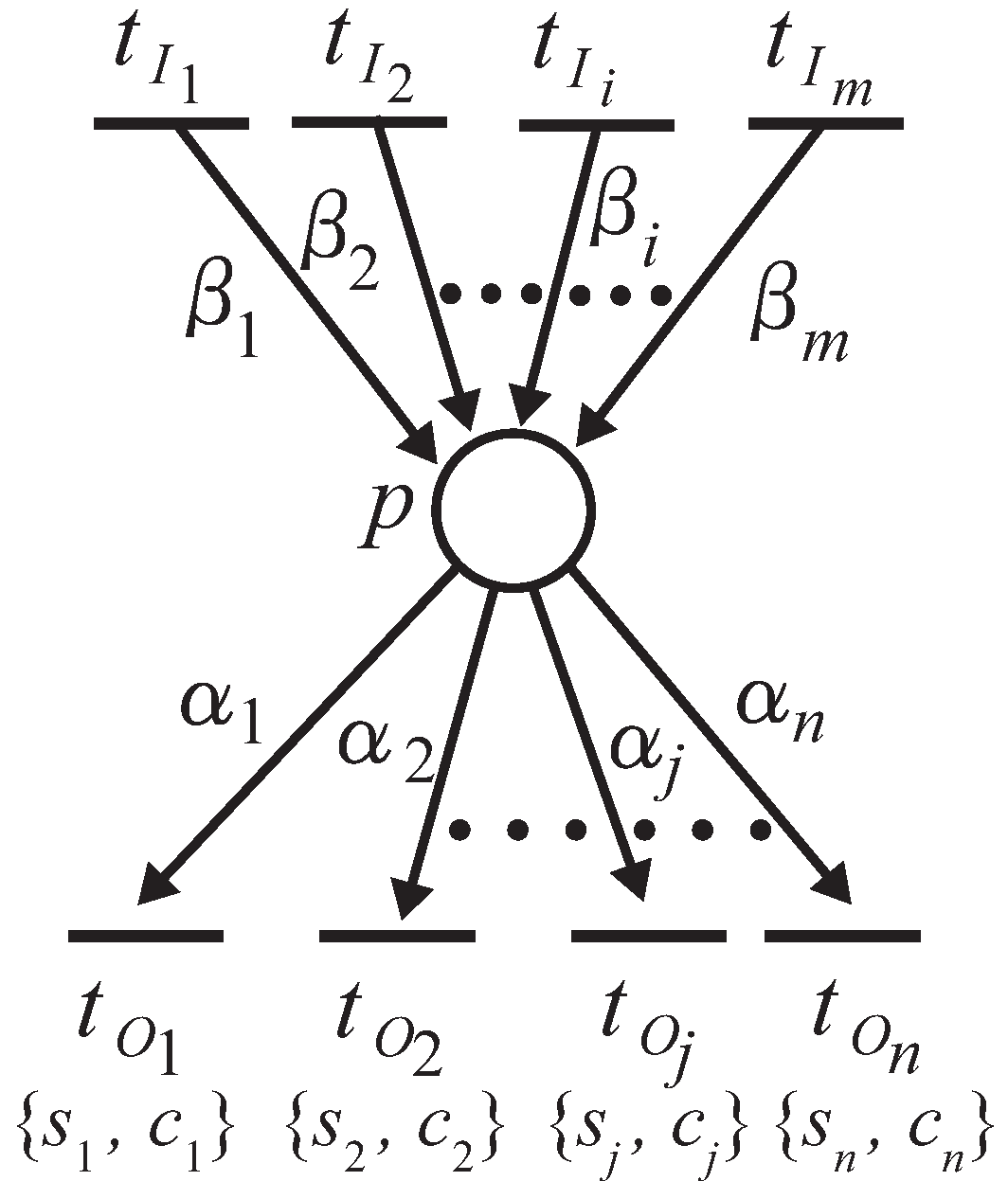
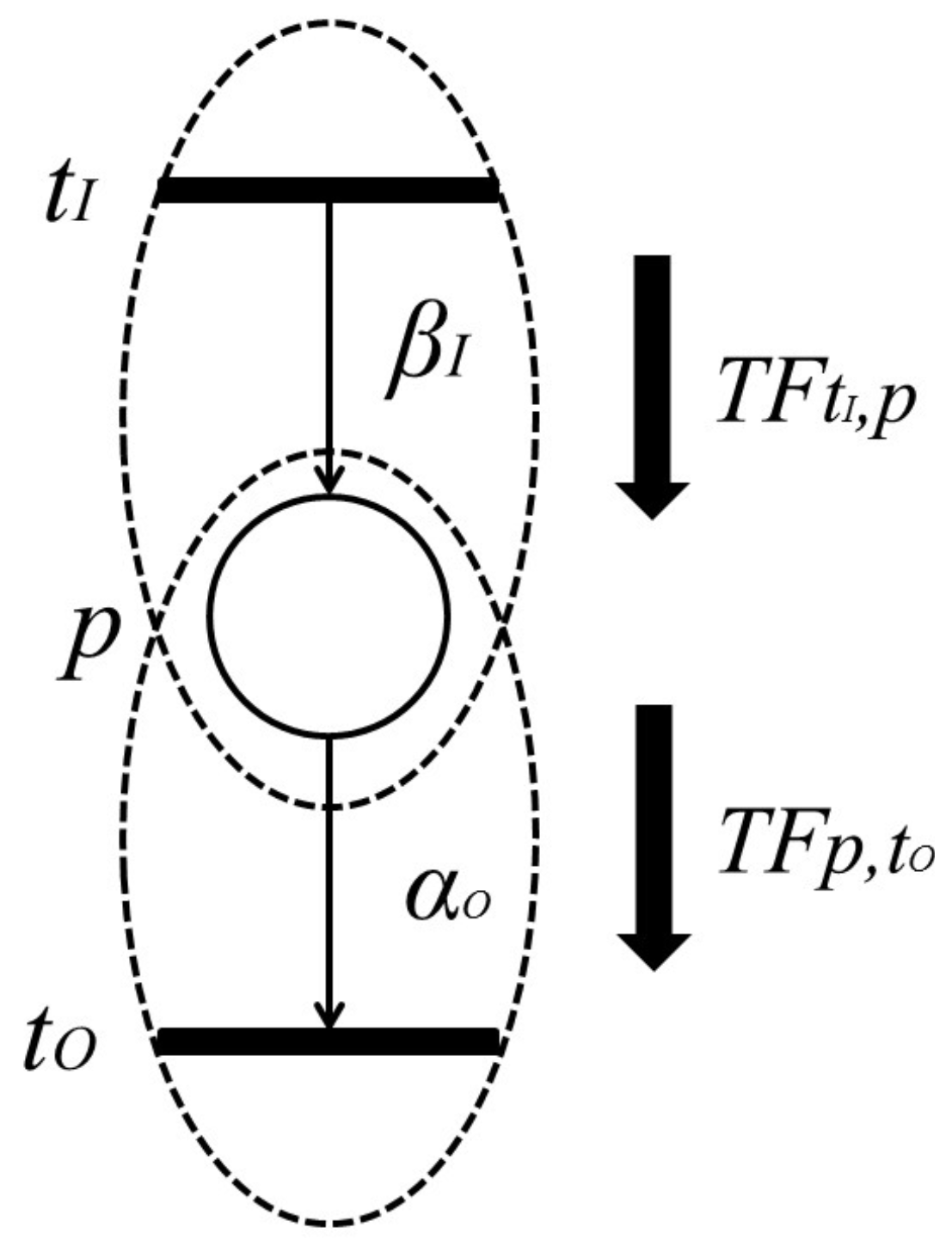
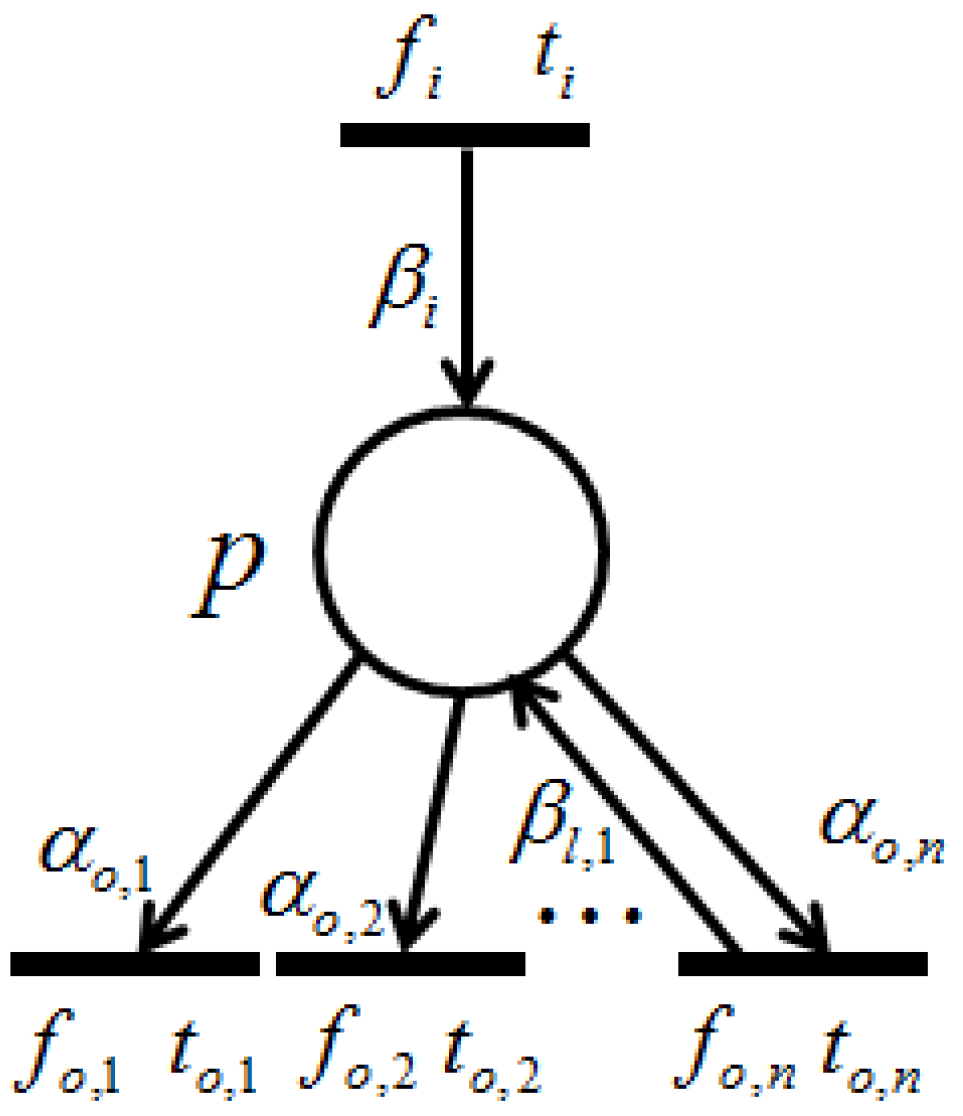
[23] With the firing of transition $t_I$, token amounts flowing into place p per unit of time are called “input token-flow” and are denoted by $T{F}_{t_I,p}$. On the other hand, with the firing of transition $t_O$, token amounts flowing out of place p per unit of time are called “output token-flow” and are denoted by $T{F}_{p,t_O}$. $T{F}_{t_I,p}$ and $T{F}_{p,t_O}$ (shown in Figure 6) are defined by the following equations, respectively:

$$\begin{array}{ccc}\hfill T{F}_{t_I,p}& =& f_I{\beta }_I\hfill \end{array}$$

(3)

$$\begin{array}{ccc}\hfill T{F}_{p,t_O}& =& f_O{\alpha }_O,\hfill \end{array}$$

(4)

where $f_I$ and $f_O$ are the firing frequencies of $t_I$ and $t_O$, respectively, and ${\beta }_I$ and ${\alpha }_O$ are the weights of $e=(t_I,p)$ and $e=(p,t_O)$, respectively.

Based on this definition, the following proposition holds.

Proposition 1.

[23] Let p be a place with input transitions $\left\{t_{I_i}\right|t_{I_i}{\in }^{•}p\}$ and output transitions $\left\{t_{O_j}\right|t_{O_j}\in p^{•}\}$. Then, ${\sum }_{i=1}^{m}T{F}_{t_{I_i},p}$ and ${\sum }_{j=1}^{n}T{F}_{p,t_{O_j}}$ are the total input token-flow and the total output token-flow for place p, respectively. Furthermore, when firing frequency f is at the maximum firing rate, $\overline{f}$, input token-flow $T{F}_{t_I,p}$ and output token flow $T{F}_{p,t_O}$ become the maximum, $\overline{F{T}_{t_I,p}}$ and $\overline{F{T}_{p,t_O}}$, respectively. These maximum token-flows satisfy the following equations.

$$\begin{array}{ccc}\hfill {\displaystyle \sum _{i=1}^m}T{F}_{t_{I_i},p}& \le & {\displaystyle \sum _{i=1}^m}\overline{F{T}_{t_{I_i},p}}\hfill \end{array}$$

(5)

$$\begin{array}{ccc}\hfill {\displaystyle \sum _{j=1}^n}T{F}_{p,t_{O_j}}& \le & {\displaystyle \sum _{j=1}^n}\overline{F{T}_{p,t_{O_j}}}\hfill \end{array}$$

(6)

The following requirement is trivial.

Proposition 2.

[23] In a timed Petri net, the total output token-flow is not more than the total input token-flow for each place p:

$$\begin{array}{c}\hfill {\displaystyle \sum _{i=1}^m}T{F}_{t_{I_i},p}\ge {\displaystyle \sum _{j=1}^n}T{F}_{p,t_{O_j}},\end{array}$$

(7)

In a signaling pathway, a reaction not only modifies the formation of molecules, as mentioned above, but also controls the amounts of produced substances. Although the amount of a substance will change along the signal propagation, it cannot be increased indefinitely; otherwise, an abnormal accumulation of a substance may cause a crucial problem in the signaling pathway. Based on this observation, we introduced the notion of a “retention-free” pathway for a timed Petri net. In a retention-free Petri net, the total token amounts flowed-in and flowed-out for each place per unit of time are equivalent.

Definition 8.

[23] A timed Petri net $TPN$ is called a retention-free Petri net ($RFPN$) (satisfying Proposition 1) if the total input token-flow and total output token-flow are equivalent at any place of $TPN$, that is,

$$\begin{array}{c}\hfill {\displaystyle \sum _{i=1}^m}T{F}_{t_{I_i},p}={\displaystyle \sum _{j=1}^n}T{F}_{p,t_{O_j}}.\end{array}$$

(8)

In fact, there exists at least one T-invariant in an $RFPN$, which indicates a firing counting vector of transitions in a periodic firing sequence [26] that leads back to the marking where it starts. This is because actually, the firing frequencies of all of the transitions construct a T-invariant.

4. Dependency Relation and Dependent Shrink

The firing frequency of a certain transition can be calculated if the firing frequencies of the transitions attached to that transition have been determined thus far, i.e., when these transitions are dependent on each other with respect to the firing frequencies. To provide a clear and precise definition of this dependency of the transitions, we introduce a new concept called a “dependency relation” for transitions, which is formalized based on the retention-free concept presented in the previous section. After that, we propose a method for shrinking a Petri net subnet, induced by the transitions satisfying a dependency relation, into a single transition. In other words, if a subnet can be shrunk, then the firing frequency of any transition in the subnet can be deduced based on the firing frequency of a certain transition inside the subnet.

4.1. Dependency Relation

Definition 9.

Let $TPN$ be a timed Petri net and $t_i$ and $t_j$ be two transitions. Here, $t_i$ and $t_j$ are said to be related to each other if and only if the following equation holds:

$$\begin{array}{c}\hfill f_i=r_{ij}{f}_j,\end{array}$$

(9)

where $f_i$ and $f_j$ are the firing frequencies of $t_i$ and $t_j$, and $r_{ij}$ is a positive rational. This is called a dependency relation and is denoted by $(t_i,t_j)\in R$.

The above equation means if two transitions are related to each other, then firing frequencies are dependent. Based on this definition, we have the following propositions.

Theorem 1.

A dependency relation is an equivalence relation.

Proof. 

We only need to prove that a dependency relation is reflexive, symmetric and transitive. Let t, $t_1$, $t_2$ and $t_3$ be transitions of a Petri net. A dependency relation is clearly reflexive and symmetric because (1) $f_t=f_t$ holds and (2) if $f_1=r_{12}{f}_2$, then $f_2=\frac{1}{r_{12}}{f}_1$, and vice versa. Suppose $f_1=r_{12}{f}_2$ and $f_2=r_{23}{f}_3$ hold, then $f_1=r_{12}{r}_{23}{f}_3$, which means the dependency relation is transitive. ☐

Based on the Definition 9, we have the following proposition for a retention-free Petri net.

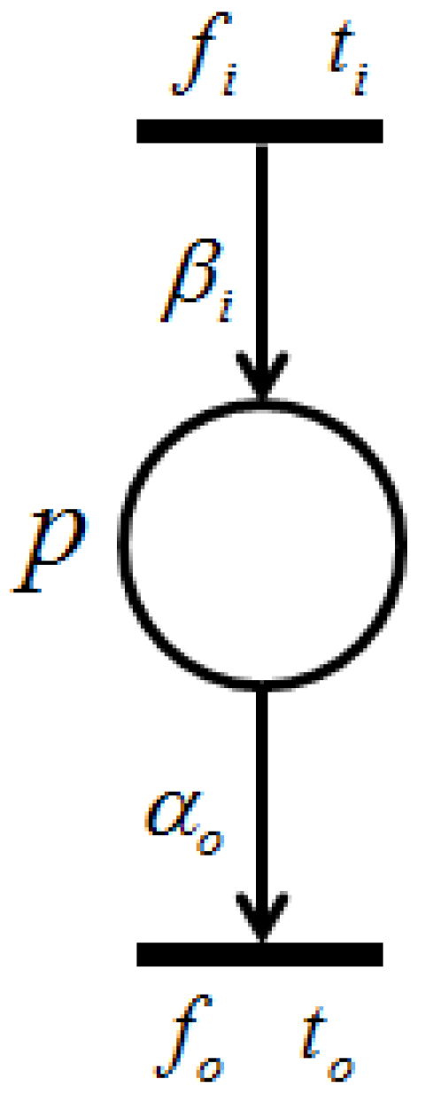
Proposition 3.

Let $P{N}_{siso}$ and $P{N}_{conf}$ be two retention-free nets consisting of a place with single input and single output transitions (called a single-input and single-output structure), and a conflict place with multiple transitions (called a conflict structure), respectively. (i) In $P{N}_{siso}$, the input transition and output transition satisfy a dependency relation; (ii) in $P{N}_{conf}$, all output transitions satisfy their dependency relation with one another.

Proof. 

(i) Suppose $P{N}_{siso}$ is a net, as shown in Figure 7. Because Figure 7 is retention free, the amount of input and output token flows through place p must be equal, i.e., $f_i{\beta }_i=f_o{\alpha }_o$. Thus, the firing frequency $f_i$ can be expressed as $f_i=\frac{{\alpha }_o}{{\beta }_i}{f}_o$. (ii) Without a loss of generality, herein we suppose place p possesses a single input transition (because we only need to consider the dependency relation of the output transitions), as shown in Figure 8.

Since the given firing probabilities of all output transitions, $s_{o,1},s_{o,2},\cdots ,s_{o,n}$, satisfy:

$$\begin{array}{ccc}\hfill \frac{s_{o,1}}{s_{o,2}}& =& \frac{f_{o,1}}{f_{o,2}}\hfill \\ \hfill \frac{s_{o,1}}{s_{o,3}}& =& \frac{f_{o,1}}{f_{o,3}}\hfill \\ & ⋮& \\ \hfill \frac{s_{o,1}}{s_{o,n}}& =& \frac{f_{o,1}}{f_{o,n}}.\hfill \end{array}$$

(10)

the firing frequencies, $f_{o,2}$, $f_{o,3}$, ⋯, $f_{o,n}$, can be expressed through the following equations:

$$\begin{array}{ccc}\hfill f_{o,2}& =& \frac{s_{o,2}}{s_{o,1}}{f}_{o,1}\hfill \\ \hfill f_{o,3}& =& \frac{s_{o,3}}{s_{o,1}}{f}_{o,1}\hfill \\ & ⋮& \\ \hfill f_{o,n}& =& \frac{s_{o,n}}{s_{o,1}}{f}_{o,1},\hfill \end{array}$$

(11)

which means that all output transitions satisfy the dependency relations with one another. ☐

The two nets shown above are elementary structures of $RFPN$, which will be applied in the following discussion, as well as in our algorithm.

As shown in Theorem 1 above, a dependency relation is an equivalence relation. Hence, the transition set of a timed Petri net can be divided into independent subsets, i.e., equivalence classes. In the following subsection, to indicate a block of a retention-free Petri net, in which all transitions satisfy a dependency relation, we provide a definition of “dependent shrink”.

4.2. Dependent Shrink

Definition 10.

Let $PN=(T,P,E,\alpha ,\beta )$ be a retention-free Petri net.

(i)

Let $T_x$ be a subset of T, where x ($1\le x\le \left|T\right|$) is a positive integer, and all of the transitions in $T_x$ satisfy a dependency relation. A Petri net induced by $T_x$ is defined as $P{N}_x=(T_x,P_x,E_x,\alpha ,\beta )$, where $P_x=\left\{p\right|p{\in }^{•}t\cup t^{•},t\in T_x\}$, and $E_x=\left\{e\right|e\in T_x\times P_x\cup P_x\times T_x\}$.

(ii)

The transformation of $P{N}_x$ by constructing all transitions of $T_x$ and any place $p\in P_x$ satisfying ${}^{•}p\cup p^{•}\subset T_x$ into a single transition, denoted by $t_x$, is called a dependent shrink. In addition, the resultant net $P{N}^{\prime }=(T^{\prime },P^{\prime },E^{\prime },\alpha ,\beta )$ transformed from $PN$ is called a dependent shrunk net, where, $T^{\prime }=T-T_x+t_x$, $P^{\prime }=P-\{p{|}^{•}p\cup p^{•}\subset T_x\}$, $E^{\prime }=\left\{e\right|e\in T^{\prime }\times P^{\prime }\cup P^{\prime }\times T^{\prime }\}$, α and β of $t_x$’s input and output arcs are decided, such that the input and output token flows of the places, included in ${}^{•}{t}_x\cup t_x^{•}$, are kept equivalent before and after shrinking.

The following lemma shows us that the dependency relation of the transitions does not change before and after a dependent shrink, i.e., if two transitions are out of the dependency relation, then they will not satisfy the dependency relation after a dependent shrink; and vice versa.

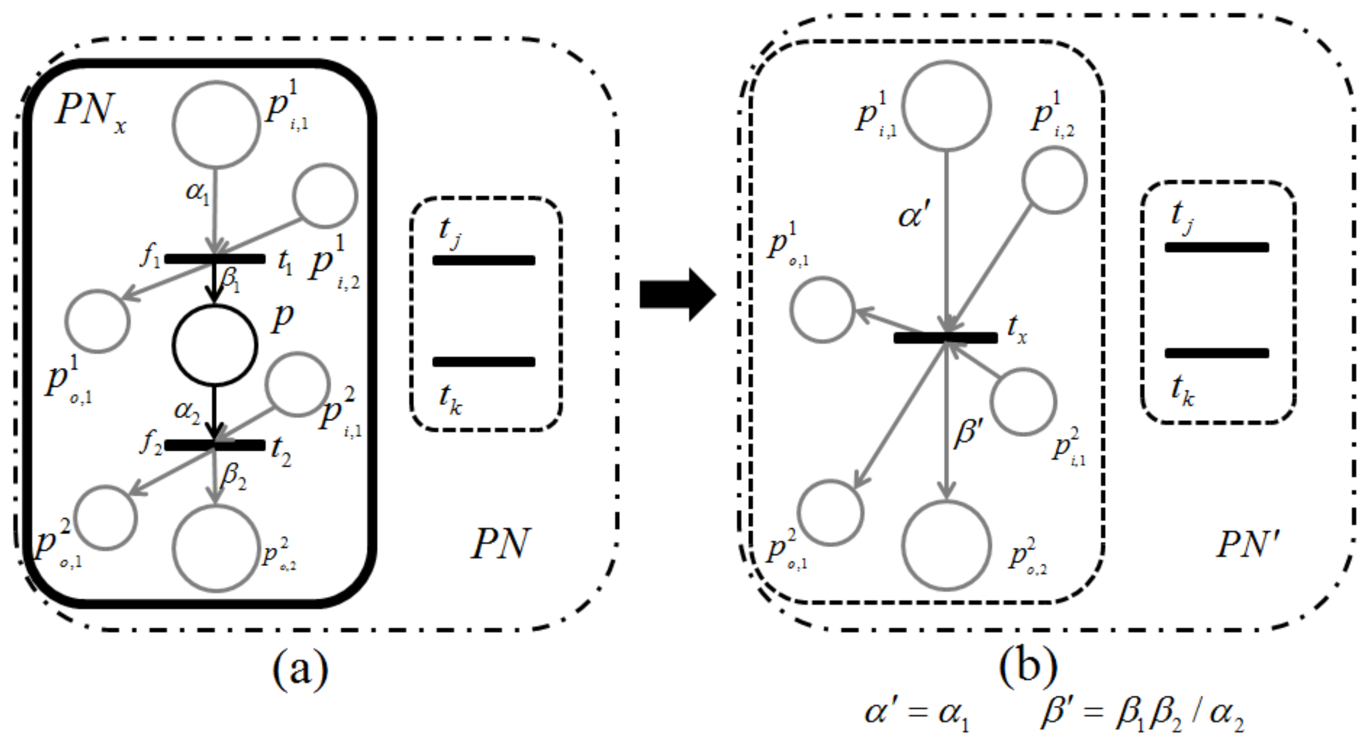
Lemma 1.

Let $PN=(T,P,E,\alpha ,\beta )$ be a retention-free net including a subnet $P{N}_x=(T_x,P_x,E_x,\alpha ,\beta )$ of Figure 9a or Figure 10a and $P{N}^{\prime }=(T^{\prime },P^{\prime },E^{\prime },\alpha ,\beta )$ be its dependent shrunk net by applying a dependent shrink for $P{N}_x$, where $T^{\prime }=T-T_x+t_x$. Suppose $t_j,t_k\in T-T_x$ and $t_y\in T_x$; then, the following claims hold.

Claim 1:

If $(t_j,t_k)\in R$ in $PN$, then $(t_j,t_k)\in R$ in $P{N}^{\prime }$; otherwise, $(t_j,t_k)\notin R$ in $P{N}^{\prime }$.

Claim 2:

If $(t_j,t_y)\in R$ $((t_k,t_y)\in R)$ in $PN$, then $(t_j,t_x)\in R$ $((t_k,t_x)\in R)$ in $P{N}^{\prime }$; otherwise, $(t_j,t_x)\notin R$$((t_k,t_x)\notin R)$ in $P{N}^{\prime }$.

Proof. 

Recall that a single-input and single-output structure (Figure 7) and a conflict structure (Figure 8) are the elementary structures of $RFPN$ considered in this paper. $P{N}_x$s surrounded by the bold line in Figure 9a and Figure 10a are basically the same as in Figure 7 and Figure 8, respectively, but these are extended by attaching additional places and arcs (pale parts) in order to make them more general. In addition, two transitions, $t_j$ and $t_k$, are appended for the proof of Lemma 1 below.

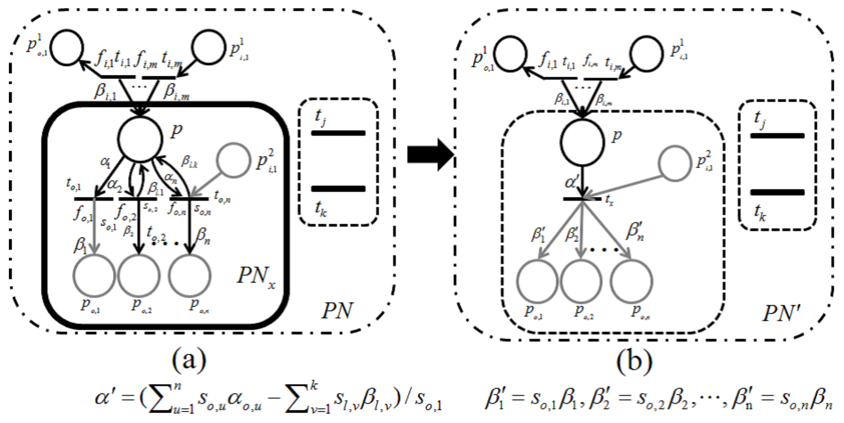
For the case of Figure 9, p and its input and output transitions ($t_1$ and $t_2$) are shrunk into a single transition, $t_x$, and the weights of the new input and output arcs are given as ${\alpha }^{\prime }={\alpha }_1$ and ${\beta }^{\prime }={\beta }_2\frac{{\beta }_1}{{\alpha }_2}$, respectively. On the other hand, for the case of Figure 10, all output transitions of place p are shrunk into a single transition, $t_x$, and the weights of the new input and output arcs are set to:

$$\begin{array}{ccc}\hfill {\alpha }^{\prime }& =& \left({\displaystyle \sum _{u=1}^n}{s}_{o.u}{\alpha }_{o.u}-{\displaystyle \sum _{v=1}^k}{s}_{l.v}{\beta }_{l.v}\right)/s_{o.1}\hfill \\ \hfill {\beta }_1^{\prime }& =& s_{o.1}{\beta }_1\hfill \\ \hfill {\beta }_2^{\prime }& =& s_{o.2}{\beta }_2\hfill \\ & ⋮& \\ \hfill {\beta }_n^{\prime }& =& s_{o.n}{\beta }_n.\hfill \end{array}$$

Here, ${\alpha }^{\prime }>0$ should be satisfied; otherwise, $PN$ is not a retention-free Petri net. For both of these two cases, the moderated tokens on ${}^{•}{t}_j\cup t_j^{•}$ and ${}^{•}{t}_k\cup t_k^{•}$ arising from the firings of $t_1$ and $t_2$ of Figure 9a and the firings of $t_{o,1},t_{o,2},\cdots ,\text{ and }{t}_{o,n}$ of Figure 10a have no changes before or after shrinking $P{N}_x$; that is, the dependency relation between $t_j$ and $t_k$ is not changed, and Claim 1 therefore holds.

Let us see Claim 2. $t_y$ should be the input or output transition of p in Figure 9 and one of the output transitions of p in Figure 10. Similar to the proof of Claim 1, the moderated tokens on ${}^{•}{t}_j\cup t_j^{•}$ and ${}^{•}{t}_k\cup t_k^{•}$ arising from the firings of $t_1$ and $t_2$ of Figure 9a and the firings of $t_{o,1},t_{o,2},\cdots ,\text{ and }{t}_{o,n}$ of Figure 10a have no changes before or after shrinking $P{N}_x$. Hence, if $(t_j,t_y)\in R$ (or $(t_k,t_y)\in R$) in $PN$, then $(t_j,t_x)\in R$ (or $(t_k,t_x)\in R$) in $P{N}^{\prime }$; oppositely, if $(t_j,t_x)\in R$ (or $(t_k,t_x)\in R$) in $P{N}^{\prime }$, then $t_j$ (or $t_k$) is related to any transition of Figure 9 or Figure 10. Therefore, this lemma holds. ☐

The changes of weights given in the proof of Lemma 1 are also applied in our proposed algorithm.

In the following subsection, the uniqueness of a dependent shrink is proven. This means that if a retention-free Petri net Q can be transformed into a dependent shrunk net, the order of transitions in Q for the transformation does not affect the final resultant net.

4.3. Uniqueness on Dependent Shrink

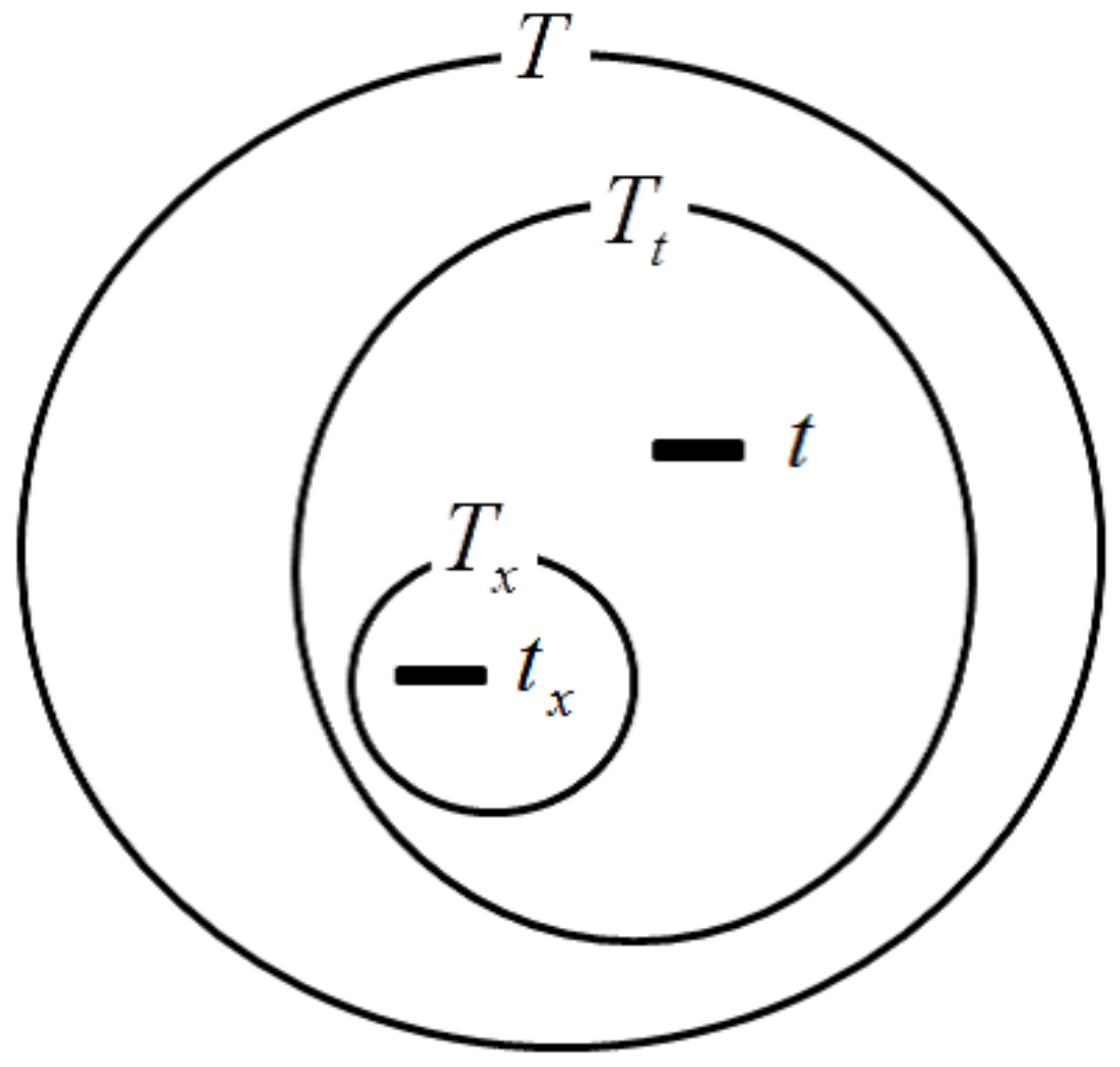
In this section, we introduce the concept of a dependent transition set that is a maximum set of transitions with a dependency relation and discuss the uniqueness of the resultant net through dependent shrink for retention-free Petri nets.

Definition 11.

Let $PN=(T,P,E,\alpha ,\beta )$ be a retention-free net, t be a transition in T and $T_t$ be a set of all transitions related to t.

(i)

Such a $T_t$ is called a t-dependent transition set.

(ii)

A Petri net induced by $T_t$ is called a t-dependent subnet and is denoted by $P{N}_t=(T_t,P_t,E_t,\alpha ,\beta )$.

Note that, differing from $P{N}_x$ defined in Definition 10, the transitions included in $P{N}_t$ are not related to any transitions of T – $T_t$ owing to the fact that $T_t$ is a maximum set of transitions with a dependency relation (shown in Figure 11). The following lemma is immediate.

Lemma 2.

Let $T_t$ and $T_{t^{\prime }}$ be the transition sets of t-dependent and t’-dependent, respectively. If $(t,t^{\prime })\in R$, then $T_t=T_{t^{\prime }}$.

Lemma 3.

Let $T_t$ be a t-dependent transition set and $P{N}_t$ be its t-dependent subnet of a retention-free Petri net $PN$. Then, $P{N}_t$ is a connected subnet.

Proof. 

Assume that $P{N}_t$ is not connected, i.e., $P{N}_t$ consists of at least two divided nets, $P{N}_1$ and $P{N}_2$. Let us see $P{N}_1=(T_1,P_1,E_1,\alpha ,\beta )$ and its connection to the other part of $PN$. There exists a subset $P_1^{\prime }\subset P_1$ of places that includes all places connecting with the outside transitions (not included in $T_1$), for instance, $T_o$. Thus, these transitions of $T_o$ are the only ones that connect $P{N}_1$ to other parts of $PN$, and further, they are not related to any one of $T_t$ ($(t_o,t)\notin R$ for $t_o\in T_o$ and $t\in T_t$); otherwise, $T_o\subset T_t$. Because $P{N}_1$ and $P{N}_2$ are not connected, any transition of $P{N}_2$ connecting to a transition of $P{N}_1$ should pass through at least one of $T_o$, which implies that the transitions of $P{N}_2$ are not related to $T_1$, and thus, this contradicts that $T_t$ is a t-dependent transition set. ☐

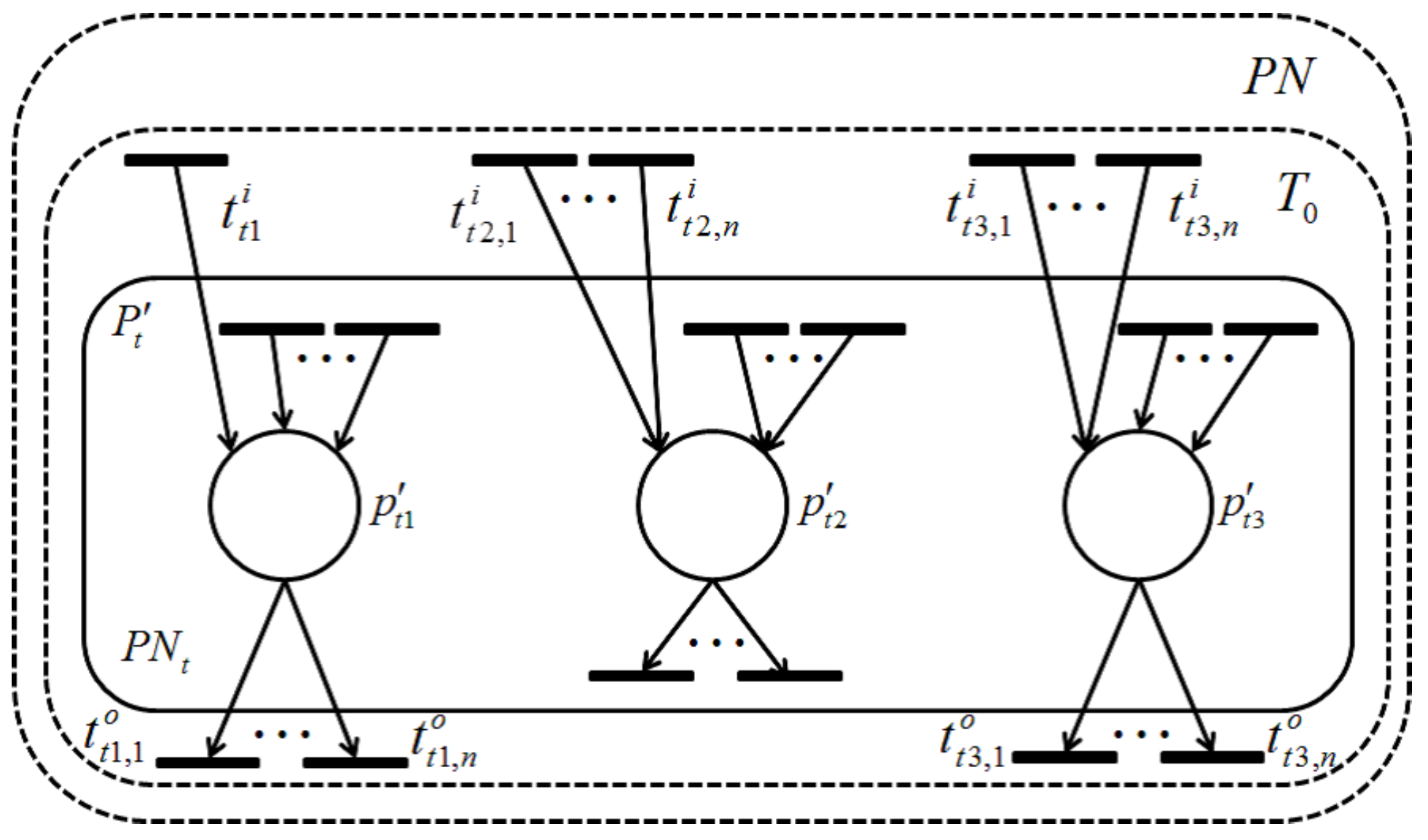
Theorem 2.

Let t be a transition of a retention-free Petri net $PN=(T,P,E,\alpha ,\beta )$, $T_t$ be a t-dependent transition set, $P{N}_t=(T_t,P_t,E_t,\alpha ,\beta )$ be a t-dependent subnet, $P{N}^{\prime }=(T^{\prime },P^{\prime },E^{\prime },\alpha ,\beta )$ be a net by shrinking $P{N}_t$ and $t_t$ be a shrunken transition of $P{N}_t$. For $t_i,t_j\notin T_t$, $(t_i,t_t)\notin R$ and $(t_j,t_t)\notin R$ are satisfied in $P{N}^{\prime }$. Further, if $(t_i,t_j)\in R$ in $PN$, then $(t_i,t_j)\in R$ in $P{N}^{\prime }$, and vice versa.

Proof. 

There exists a subset $P_t^{\prime }\subset P_t$ of places that includes all places connecting with the outside transitions (not included in $T_t$), for example, $T_o$. Thus, these transitions of $T_o$ are only those that connect $P{N}_t$ to other parts of $PN$, and further, they are not related to any of $T_t$ ($(t_o,t)\notin R$ for $t_o\in T_o$ and $t\in T_t$); otherwise, $T_o\subset T_t$. After shrinking $P{N}_t$, $P_t^{\prime }$ and $t_t$ remain in $P{N}^{\prime }=(T^{\prime },P^{\prime },E^{\prime },\alpha ,\beta )$, and of course, $(t_o,t_t)\notin R$ holds in $P{N}^{\prime }$ for $t_o\in T_o$. Further, any transition $t^{\prime }$ included in $T^{\prime }-\left\{t_t\right\}$ connecting to $t_t$ should pass through at least one of $T_o$, which means that $(t_i,t_t)\notin R$ and $(t_j,t_t)\notin R$ hold for $t_i,t_j\notin T_t$. Furthermore, shrinking $P{N}_t$ does not destroy the dependency relation for any transitions of $T_o$, as can be seen in Figure 12 and Figure 13 and, thus, for the transitions of $T^{\prime }-T_o-\left\{t_t\right\}$. Therefore, this theorem holds. ☐

According to Theorem 2, if we find all dependent subnets and shrink them individually into single transitions, then all of these transitions are representative of the equivalence classes because a dependency relation is an equivalence relation. The following corollary is immediate.

Corollary 1.

Suppose a retention-free Petri net $PN$ consists of k subnets, $P{N}_{t_1},P{N}_{t_2},\cdots ,P{N}_{t_k}$, each of which is a dependent subnet. Not depending on the order of dependent shrink for $P{N}_{t_1},P{N}_{t_2},\cdots ,P{N}_{t_k}$, a unique structure of a resultant net consisting of k transitions can be obtained.

From Lemma 1 and Theorem 2, we can simply obtain the following result.

Corollary 2.

Iterating a dependent shrink for the cases shown in Figure 9 and Figure 10, a unique resultant net can be obtained.

5. Dependent Shrink Algorithm and Case Study

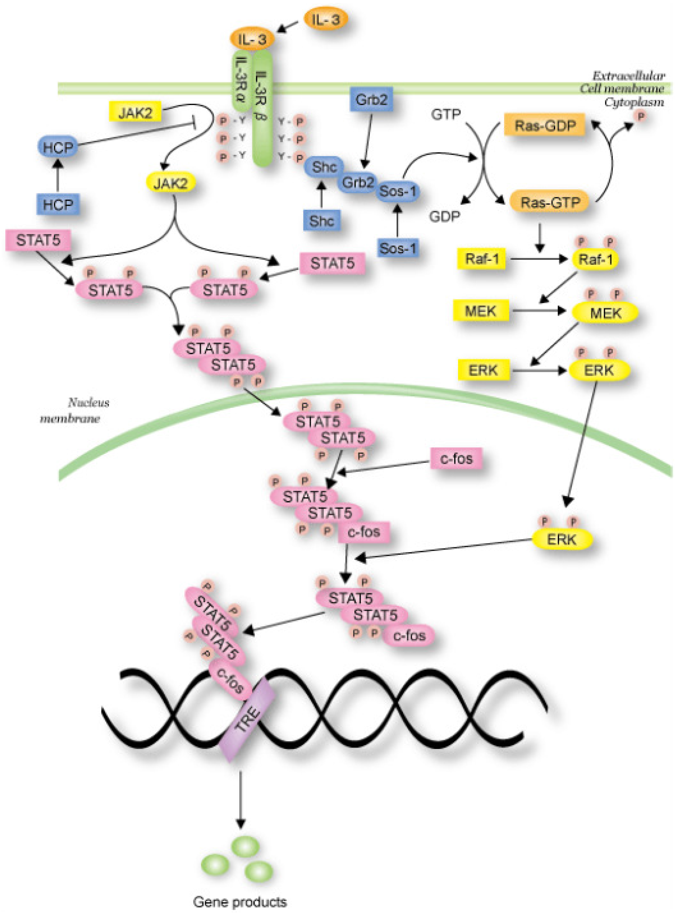
In this section, we propose the dependent shrink algorithm based on the discussion in the last section and apply this algorithm to the IL-3 signaling pathway Petri net model (shown in Figure 15), which is transformed from the IL-3 phenomenon model (shown in Figure 14) obtained from the website [27], as a case study. Note that IL-3 is a glycoprotein and is known to be involved in the immune response [28,29,30].

5.1. Outline of Shrink Process

The outline of the dependent shrink process can be briefly described as follows:

Step 1:

Shrinking of self-loop structure:

A place randomly selected from a Petri net is stored in a queue after the conversion of the self-loops and the structures of conflict (as shown in Figure 10).

Step 2:

Shrink of conflict structure:

If a place picked up from the queue has a self-loop or a transition of one-input and one-output (as shown in Figure 9), this place is shrunk.

Step 3:

Changing weight of the input arc:

If a shrunk Petri net has a place with multiple input transitions, then enqueue and continue to Step 2. This procedure is repeated until the queue becomes empty or the number of places with multiple input transitions equals the length of the queue.

The variables used in the algorithm are as follows:

• $P{N}_0$ is a given signaling pathway Petri net model constituted by $T_0,P_0,and{E}_0$.
• N is a variable that stores the Petri net after dependent shrink, constituted by $T,P$ and E.
• Q is a queue.
• X is a set of places initially set as a given place set, $P_0$.
• f is a flag by which a dependent shrink pattern is determined.
• c is a counter, which counts the number of places in Q with multiple input transitions.

5.2. Dependent Shrink Algorithm

The following algorithm is used to repeatedly shrink the structures of Figure 9 and Figure 10 to find transitions with an interdependent firing frequency.

Algorithm 1 Dependent Shrink

Input: $P{N}_0=(T_0,P_0,E_0)$

Output: Shrunk Petri net $N=(T,P,E)$

Main $\left(P{N}_0\right)$

$1^{\circ }$ $T\leftarrow T_0$, $P\leftarrow P_0$, $E\leftarrow E_0$, $N\leftarrow (T,P,E)$

$2^{\circ }$ $X\leftarrow P$, $Q\leftarrow \varphi$, $c\leftarrow 0$

$3^{\circ }$ while ($X\ne \varphi$)

Pull an element x from $X(X\leftarrow X-\{x\left\}\right)$

Enqueue($Q,x$)

Shrink1($N,x$)

$4^{\circ }$ Shrink2($N,Q,c$)

Shrink1($N,x$)

$1^{\circ }$ if ($|{}^{•}x\cap x^{•}|\ge 1$) then

$f\leftarrow 1$

Arcweight$(N,x,f)$

$2^{\circ }$ if ($|x^{•}|\ge 2$) then

$f\leftarrow 2$

Arcweight($N,x,f$)

Shrink2($N,Q,c$)

$1^{\circ }$ while $\left(\right|Q|\ge 1)$

$x\leftarrow \mathbf{Dequeue}\left(Q\right)$

if ($|{}^{•}x\cap x^{•}|\ge 1$) then

$f\leftarrow 1$

Enqueue $(Q,x)$

$c\leftarrow 0$

else if ($|{}^{•}x|=|x^{•}|=1$) then

$f\leftarrow 3$

$c\leftarrow 0$

else if ($|{}^{•}x|\ge 2$) then

$f\leftarrow 4$

Enqueue(Q, x)

$c\leftarrow c+1$

if ($f\ne 4$) then

Arcweight($N,x,f$)

if ($c=\left|Q\right|$) then

Break

Arcweight($N,x,f$)

$1^{\circ }$ if ($f=1$) then

$\forall t^{\prime }\in {}^{•}x\cap x^{•}$

$\alpha (x,t^{\prime })=\alpha (x,t^{\prime })-\beta (t^{\prime },x)$

if ($\alpha (x,t^{\prime })<0)$ then

$\beta (t^{\prime },x)=\left|\alpha (x,t^{\prime })\right|$

$E\leftarrow E-\left\{(x,t^{\prime })\right\}$

else if ($\alpha (x,t^{\prime })>0$) then

$E\leftarrow E-\left\{(t^{\prime },x)\right\}$

else if ($\alpha (x,t^{\prime })=0$) then

$E\leftarrow E-\{(t^{\prime },x),(x,t^{\prime })\}$

$2^{\circ }$ else if ($f=2$) then

$T\leftarrow T\cup \left\{t^{\prime }\right\}$

$E\leftarrow E\cup \left\{(x,t^{\prime })\right\}\cup \left\{(u,t^{\prime })\right|u\in {}^{•}z,z\in x^{•}\}\cup \left\{(t^{\prime },v)\right|v\in z^{•},z\in x^{•}\}$

Choose $z^{\prime }\in x^{•}$.

$\forall z\in x^{•}-\left\{t^{\prime }\right\}$

$\alpha (x,t^{\prime })=\alpha (x,t^{\prime })+s\left(z\right)*\alpha (x,z)$

$\forall v\in z^{•},z\in x^{•}$

$\beta (t^{\prime },v)=s\left(z\right)*\beta (z,v)$

$\forall u\in {}^{•}z,z\in x^{•}$

$\alpha (u,t^{\prime })=s\left(z\right)*\alpha (u,z)/s\left(z^{\prime }\right)$

$\alpha (x,t^{\prime })=\alpha (x,t^{\prime })/s\left(z^{\prime }\right)$

$T\leftarrow T-\left\{z\right|z\in x^{•}-\left\{t^{\prime }\right\}\}$

$3^{\circ }$else if ($f=3$) then

$T\leftarrow T\cup \left\{t^{\prime }\right\}$

Let $z_i,z_o$ be $\left\{z_i\right\}={}^{•}x$, $\left\{z_o\right\}=x^{•}$ (due to $|{}^{•}x|=|x^{•}|=1$).

$E\leftarrow E\cup \left\{(u,t^{\prime })\right|u\in {}^{•}{z}_i\cup {}^{•}{z}_o\}\cup \left\{(t^{\prime },v)\right|v\in z_i^{•}\cup z_o^{•}\}$

$\forall u\in {}^{•}{z}_i$

$\alpha (u,t^{\prime })=\alpha (u,z_i)$

$\forall u\in {z_i}^{•}$

$\beta (t^{\prime },u)=\beta (z_i,u)$

$\forall v\in {}^{•}{z}_o$

$\alpha (v,t^{\prime })=\beta (z_i,x)*\alpha (v,z_o)/\alpha (x,z_o)$

$\forall v\in {z_o}^{•}$

$\beta (t^{\prime },v)=\beta (z_i,x)*\beta (z_o,v)/\alpha (x,z_o)$

$T\leftarrow T-\left\{z_i\right|z_i\in {}^{•}x\}-\left\{z_o\right|z_o\in x^{•}\}$

$P\leftarrow X-\left\{x\right\}$

The Algorithm 1 will terminate when all places are shrunk, i.e., a single transition remains, or becomes ones with multiple input transitions and a single output transition. The time complexity is $O\left(\right|P\left|\right|E\left|\right)$. As a result, given with a retention-free Petri net, this algorithm gives a smaller shrunk net, in which a transition may represent a class of ones with a dependency relation.

5.3. Case Study

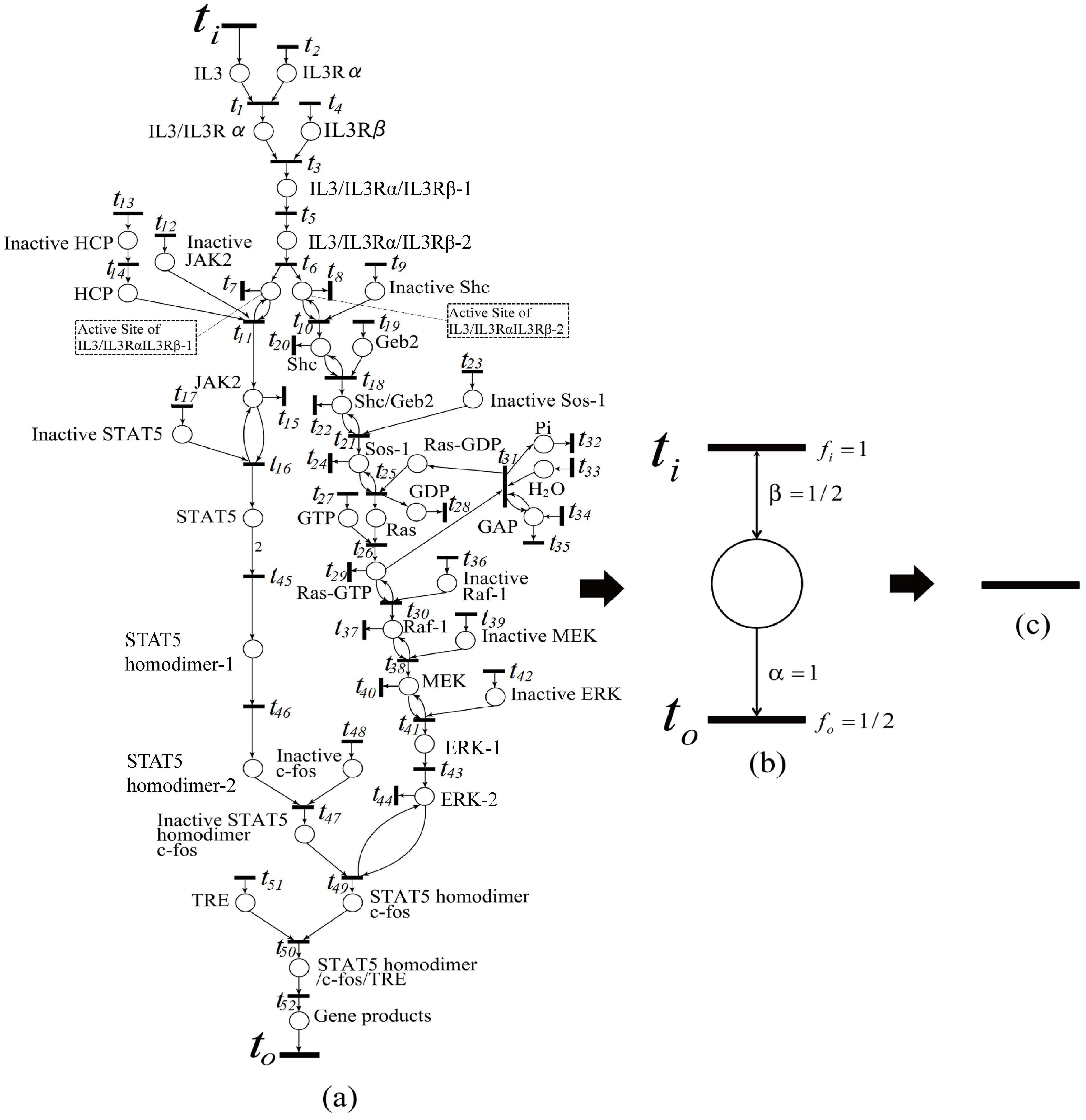
Here, we give an example showing an application of our proposed algorithm. Since the algorithm has not been implemented, here we manually apply it. The algorithm is applied to the IL-3 Petri net model (see Figure 15a), obtained from the website [27]. As a result, the original IL-3 Petri net model shown in Figure 15a is shrunk into Figure 15c. This means that the firing frequencies of all transitions in Figure 15a are dependent on one another. In the intermediate shrunk net (see Figure 15b), by assuming that the firing frequency $f_i$ of the input transition $t_i$ is one, and the weights of the input and output arcs are $\frac{1}{2}$ and one, respectively, then the firing frequency $f_o$ of output transition $t_o$ is $\frac{1}{2}$. In this way, we can calculate all firing frequencies in the IL-3 Petri net model if the firing frequency of one transition is known in this model.

That is, all of the reaction speed data of the IL-3 Petri net model are dependent on one another, and thus, if one reaction speed datum is available, all of the others can be derived from it.

We have two ways to determine reaction speed data in biological pathway, i.e., firing frequencies. One is to find firing frequency relationships between transitions from the intermediate shrunk nets generated during the execution of the Algorithm 1, in turn from the final net to the original net.

In the intermediate shrunk net (see Figure 15b), by assuming the firing frequency $f_i$ of the input transition $t_i$ to be available (say one), then the firing frequency $f_o$ of output transition $t_o$ is $\frac{1}{2}$. Recursively, we can derive all of the firing frequencies in the IL-3 Petri net model.

Another way is to establish a series of linear equations for all of the places according to retention-freeness, Equation (8), and to solve these equations to finally get the solutions with the form $f_{nonvalid}=r_{nonvalid,valid}{f}_{valid}$. Here, $f_{nonvalid},f_{valid}$ are the firing frequencies corresponding to non-valid and valid reaction speed data.

Suppose $t_i$ is only one transition whose corresponding speed data are valid; we can derive the firing frequencies for all of the other transitions of the IL-3 Petri net model in any one of two ways as follows:

$$\begin{array}{c}\begin{array}{ccc}\hfill f_i& =\hfill & \hfill f_1=f_2=\cdots =f_{28}=1\\ \hfill f_{29}& =\hfill & \hfill f_{30}=\cdots =f_{50}=f_o=\frac{1}{2}.\end{array}\end{array}$$

(12)

In addition to IL-3, we also apply our algorithm to the endocytosis Petri net model and give the shrunk result as can be found in the Supplementary Materials, in which, IL-3 and endocytosis respectively consist of 43 places, 54 transitions and 109 arcs and 24 places, 34 transitions and 70 arcs. Moreover, the System Biology Markup Language (SBML) [31] and Petri Net Markup Language (PNML) [32] files of those Petri net models can also be obtained from the Supplementary Materials.

5.4. Discussion on the Resultant Structure from the Algorithm

As mentioned, when the Algorithm 1 terminates, there are two possible cases: (1) the resultant net is a single transition; (2) the resultant net is such that all places possess a single output transition and multiple input transitions.

Case (1) indicates that all transitions of the given net $PN$ satisfy a dependency relation, and they comprise an equivalence class, that is, if the firing frequency of any one of the transitions is decided, then the frequencies of all of the others are automatically decided as well.

Case (2) may be further divided into: (i) the remaining net consisting of only such transitions that do not satisfy dependency relations with one another; and (ii) some of the transitions satisfying a dependency relation, but not having been shrunk into a single transition.

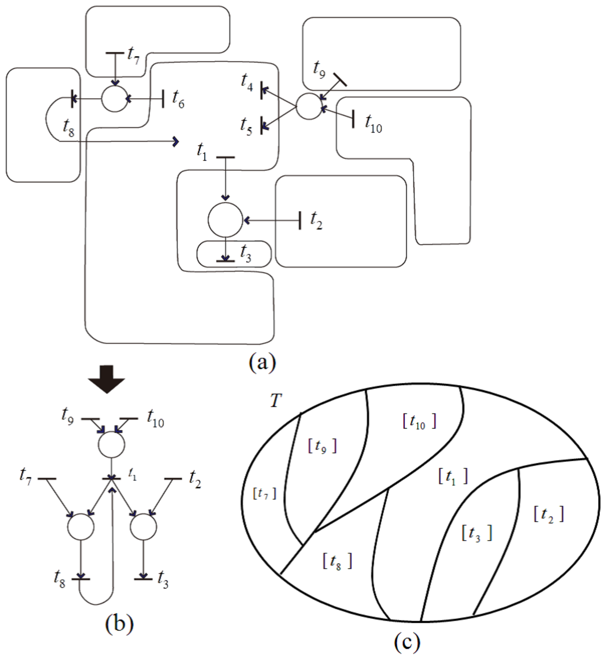
Case (2) (i) indicates that all transitions in the remaining net are independent, and each is a representative of an equivalence class, as can be illustrated in Figure 16. In this Figure 16a, each transition set is rounded by a line, and the transitions included in each set satisfy a dependency relation with one another. Applying dependent shrink, the transformed net is obtained as shown in Figure 16b. Further, the equivalence classes of $PN$ represented by $t_1,t_2,t_3,t_7,t_8,t_9,t_{10}$ are shown in Figure 16c.

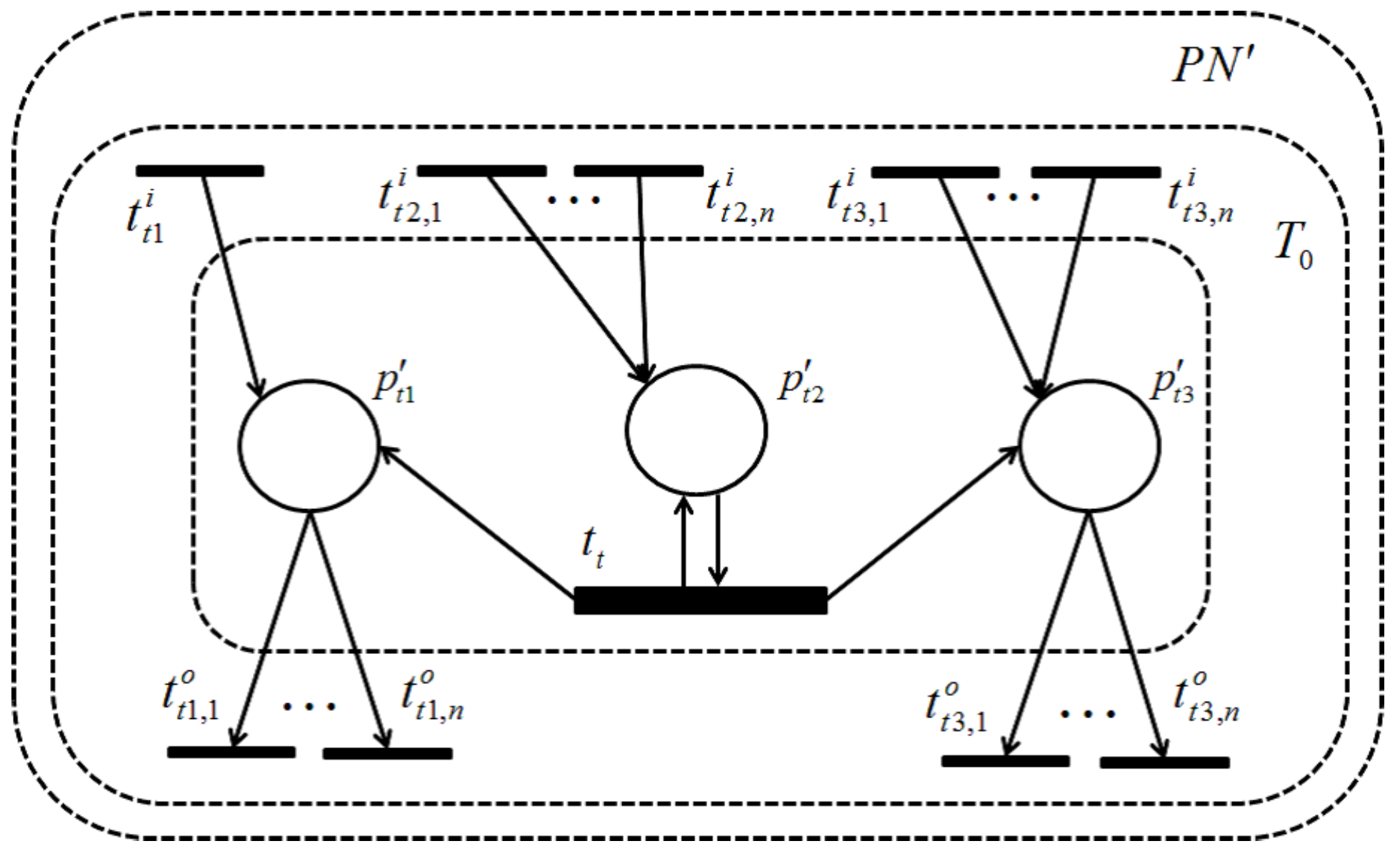
Case (2) (ii) implies that the remaining net includes a subnet that consists of transitions that all have a dependent relation, but cannot be shrunk into a single transition by shrinking the single-input and single-output structure (Figure 7) or the conflict structure (Figure 8). $P{N}_{t_2}^{\prime }$, shown in Figure 17, is such a subnet, where each transition has at least one input place with one output, which means $|P_{t_2}^{\prime }|\ge |T_{t_2}^{\prime }|$ in $P{N}_{t_2}^{\prime }$. To find such a subnet, we should establish a series of linear equations for all places according to the retention-freeness in which the input and output token flows are equal and solve these equations. Because $|P_{t_2}^{\prime }|\ge |T_{t_2}^{\prime }|$ in $P{N}_{t_2}^{\prime }$, the number of equations is more than that of the variables (firing frequencies of the transitions). Thus, if there are exactly $|T_{t_2}^{\prime }|-1$ linear independent equations, then all of the transitions satisfy a dependency relation. A detailed discussion of this remains as a future issue.

6. Conclusions

Despite the recent rapid progress in high throughput measurements of biological data, it is still difficult to gather all reaction speed data in the biological pathways. Particularly for signaling pathways, owing to their complex structure, including protein formations and enzyme reactions, computational methods are essential to estimate as much reaction data as possible from biologically-valid data. In this paper, we presented an algorithm to shrink the transitions in a timed Petri net model into a smaller number of transitions based on their dependency with respect to the firing frequency and, equally, their amount of delay.

We have first introduced a new concept, called the dependency relation, over a set of transitions of a Petri net model representing a signaling pathway, which is in fact an equivalence relation over transitions. Through a structural analysis, we obtained several properties, one important result of which is that shrinking a connected subnet, induced by transitions with a dependency relation, into a transition never affects other parts of a Petri net. Based on these results, we designed an Algorithm 1 with time complexity $O\left(\right|P\left|\right|E\left|\right)$ to reduce the Petri net size by applying a dependent shrink process for two elementary structures, i.e., a “single-input and single-output structure” and a “conflict structure”, in order to efficiently find a transition set with a dependency relation. A case study was conducted by applying our algorithm to the signaling pathway Petri net model of IL-3, and as a result, IL-3 finally becomes a single transition, which means that all reaction speeds of IL-3 are dependent on one another and that measuring one reaction speed can help in deriving all other speeds.

Our proposed method can be applied not only to signaling pathways, but also to other biological pathways in which retention-freeness holds, for example to metabolic pathways. If, in a timed Petri net model constructed from such a biological pathway, there exists a transition violating retention-freeness, then some discrepancy should happen in the biological pathway, i.e., missing interaction and/or extra interaction, which will be caused by mutations or alternations to the pathway. Such a biological inconsistency is expected to be found with our technique.

We have also pointed out that there may remain some subnets with a dependency relation in the resultant net after applying Algorithm 1 because only a dependent shrink of a “single-input and single-output structure” and a “conflict structure” are adopted. We indicated that this can be resolved by solving a series of linear equations for such a subnet without taking up too much computation time because the size of the subnet should be much smaller compared with the original net. As future work, we are planning to: (1) develop a method to find such a subnet that includes only the places possessing a single-output and multiple-input transitions with a dependency relation; (2) design an algorithm to find the transitions with a dependency relation from the solution of a series of the prior mentioned linear equations; (3) extend our method to a stochastic Petri net by taking into account probabilistic firing delay times.