Abstract
Background: The modeling of Biological Regulatory Networks (BRNs) relies on background knowledge, deriving either from literature and/or the analysis of biological observations. However, with the development of high-throughput data, there is a growing need for methods that automatically generate admissible models. Methods: Our research aim is to provide a logical approach to infer BRNs based on given time series data and known influences among genes. Results: We propose a new methodology for models expressed through a timed extension of the automata networks (well suited for biological systems). The main purpose is to have a resulting network as consistent as possible with the observed datasets. Conclusion: The originality of our work is three-fold: (i) identifying the sign of the interaction; (ii) the direct integration of quantitative time delays in the learning approach; and (iii) the identification of the qualitative discrete levels that lead to the systems’ dynamics. We show the benefits of such an automatic approach on dynamical biological models, the DREAM4(in silico) and DREAM8 (breast cancer) datasets, popular reverse-engineering challenges, in order to discuss the precision and the computational performances of our modeling method.
1. Introduction
With both the spread of numerical tools in every part of daily life and the development of NGS methods (Next Generation Sequencing methods), like DNA microarrays in biology, a very large amount of time series data is now produced [1,2,3]. This means that the produced data from the experiments on biological systems grows drastically. The newly-produced data, as long as the associated noise does not raise an issue with regard to the precision and relevance of the corresponding information, can give us some new insights into the behavior of a system. This justifies the urge to design efficient methods for inference.
Reverse engineering of gene regulatory networks from expression data have been handled by various approaches [4,5,6,7,8]. Most of them are only static. However, other researchers are rather focusing on incorporating temporal aspects in inference algorithms. The relevance of these various algorithms has been recently assessed in [9]. The authors of [10] tackled the inference problem of time-delayed gene regulatory networks through Bayesian networks, and in [11], the authors infer a temporal Boolean network. As this is a complex problem, in [12], the authors propose a time-window-extension technique based on time series segmentation in different successive phases. These approaches take gene expression data into account as the input and generate the associated regulations. However, the discrete approaches that simplify this problem by abstractions need to determine the relevant thresholds of each gene to define its active and inactive state. Various approaches have been designed to tackle the discretization problem. We can cite for example [12], in which the authors have proposed an alternative methodology that considers not a concentration level, but the way the concentration changes (in other words: the derivative of the function giving the concentration w.r.t. time) in the presence/absence of one regulator. On the other hand, the major problem for modeling lies in the quality of the expression data. Indeed, noisy data may be the main origin of the errors in the inference process. Thus, the pre-processing of the biological data is crucial for the pertinence of the inferred relations between components. In our work, we assume that the input data are pre-processed into reliable discretized time series data and focus on the dynamical inference problematics.
In this paper, we aim to provide a logical approach to tackle the learning of qualitative models of biological dynamical systems, like gene regulatory networks. In our context, we assume the set of interacting components as fixed, and we consider the learning of the interactions between those components. As in [13], in which the authors targeted the completion of stationary Boolean networks, we suppose that the topology of the network is given, providing us the influences among each gene as the background knowledge. From time series data of the evolution of the system, given its topology, we learn the dynamics of the system. The main originality of our work is that we address this problem in a timed setting, with quantitative delays potentially occurring between the moment an interaction is activated and the moment its effect is visible.
During the past decade, there has been a growing interest for the hybrid modeling of gene regulatory networks with delays. These hybrid approaches consider various modeling frameworks. In [14], the authors hybridize Petri nets: the advantage of the hybrid approach with regard to discrete modeling lies in the possibility of capturing biological factors, e.g., the delay for the transcription of RNA polymerase. The merits of other hybrid formalisms in biology have been studied, for instance timed automata [15], hybrid automata [16], the hybrid model of a neural oscillator [17] and Boolean representation [18,19]. In [20], the authors also propose algorithms to learn the delayed dynamics of systems from time series data. However, they focus only on synchronous dynamics, and the delays they consider are different from the duration of the reaction that we model here. Other works based on approximate bisimulations [21] present a procedure to compare neural structures among them, which is verified on continuous time recurrent neural networks. In addition, an application of the framework of approximate bisimulations to an approximation of nonlinear systems was proposed in [22]. Here, the authors use an over-approximation of the observational distance between nondeterministic nonlinear systems. Finally, in [23], the authors investigate a direct extension of the discrete René Thomasmodeling approach by introducing quantitative delays. These delays represent the compulsory time for a gene to turn from a discrete qualitative level to the next (or previous) one. They exhibit the advantage of such a framework for the analysis of mucus production in the bacterium Pseudomonas aeruginosa. The approach we propose in this paper inherits from this idea that some models need to capture these timing features.
Similar concerns are presents in the work of [24], where the authors model the dynamics of the system using the paradigm [25] via delayed discrete automaton and persistent entropy. However, where they focus on the global dynamics of the system, we aim to capture the local interactions of each components. Their methods can reproduce the global evolution of the system among steady states, but what we target is the precise evolution of the system every fixed amount of time.
The first theoretical steps behind our method have been introduced in [26]. In the current paper, we have deepened our work to widen its applicability: after introducing a range of filters to curate the models resulting from our algorithms, we show its efficiency on new benchmarks coming from DREAM Challenges.
We briefly introduce Automata Networks (AN) in Section 2, and all theoretical and practical notions are then settled to introduce our timed extension of AN in Section 3. Then, in Section 4, we present the related learning algorithm. We propose in Section 5 new refinement methods applied to the generated model. We demonstrate the performance of our algorithm by a running case study example in Section 6. Then, we show in Section 7 the implementation of the modeling method and of all filters in Answer Set Programming (ASP). Finally, we illustrate the merits of our approach in Section 8 by applying it on popular reverse-engineering challenges: the DREAM4 in silico dataset, then on the real data of the breast cancer network from DREAM8 dataset. Additionally, we summarize our contribution in Section 9 and give some perspectives for future works.
2. Automata Networks
We present in this section the definition and the semantics of automata networks. The enrichment of the automata networks with delays and the corresponding new semantics are presented in Section 3.
Definition 1 introduces the Automata Network (AN) [27,28,29] as a model of finite-state machines having transitions between their local state conditioned by the state of other automata in the network. A local state of an automaton is noted by , where a is the automaton identifier, and i is the expression level within a. At any time, each automaton has exactly one active local state, and the set of active local states is called the global state of the network.
The concurrent interactions between automata are defined by a set of local transitions. Each local transition has this form , with , being local states of an automaton a called, respectively, the origin and destination of τ, and ℓ is a (possibly empty) set of local states of automata other than a (with at most one local state per automaton).
Notation: Given a finite state A, is the power set of A. Given a network N, is the state of N at a time step .
Definition 1 (Automata Network (AN)).
An automata network is a triple where:
- is the finite set of automata identifiers;
- For each , , is the finite set of local states of automaton a; is the finite set of global states and denotes the set of all of the local states.
- , where with , is the mapping from automata to their finite set of local transitions.
Example 1.
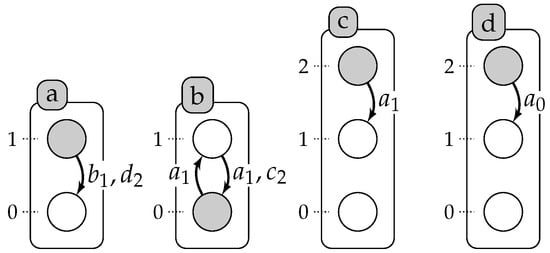
Figure 1 represents an automata network, , with four automata (), such that , , and , and five local transitions, , , , , .
Figure 1.
Example of an automata network with four automata: a, b, c and d presented by labeled boxes; and their local states are presented by circles (for instance, a is either at Level 0 or 1). A local transition is a labeled directed edge between two local states within the same automaton: its label stands for the set of necessary conditions for local states of the automata to play the transition. The grayed circles stand for the global state: .
A global state of a given AN consists of a set of all active local states of each automaton in the network. The active local state of a given automaton in a state is denoted . For any given local state , we also note if and only if . For each automaton, it cannot have more than one active local state at one global state.
Definition 2 (Playable local transition).
Let be an automata network and , with . We denote the set of playable local transitions in at time step t by: = { ∣∧ with }.
The dynamics of the AN is performed thanks to the global transitions. Indeed, the transition from one state to its successor is satisfied by a set of the playable local transitions (Definition 2) at .
Definition 3 (Global transitions).
Let be an automata network and , with and . Let be the set of playable local transitions at t. We denote the power set of global transitions at t:
In the semantics that we base our work on, the parallel application of local transitions in different automata is permitted, but it is not enforced. Thus, the set of global transitions is a power set of all of the playable local transitions (also the empty set).
3. Timed Automata Networks
In some dynamics, it is crucial to have information about the delays between two events (two states of an ). The discrete transitions, described above, cannot exhibit this information: we just process chronological information that the state will be after in the next step, but it is not possible to know chronometry, i.e., how much time this transition takes to occur and whether it blocks some transitions during this time. In fact some local transitions could not be played any more because of conflict about shared resources (necessary components to play a transition) between them. Thus, we need to restrain the general dynamics to capture more realistic behavior w.r.t. biology. Therefore, we propose in this section to add the delays in the local transitions’ attributes: timed local transitions. Later, we give the associated semantics that we base our work on to learn biological networks.
Definition 4 (Timed Automata Network (T-AN)).
A timed automata network is a triple where:
- is the finite set of automata identifiers;
- For each , , is the finite set of local states of automaton a; is the finite set of global states; denotes the set of all of the local states.
- , where with , is the mapping from automata to their finite set of timed local transitions.
To model biological networks where quantitative time plays a major role, we will use T-AN. This formalism enriches AN model with timed local transitions: . In the latter, δ is called a delay and represents the time needed for the transition to be performed. When modeling a regulation phenomenon, this allows one to capture the delay between the activation order of the production of the protein and its effective synthesis, as well as the synthesis of the product.
We note and , , and .
Lemma 1.
If is an AN, so it can be transformed to a T-AN, such that with , , and .
According to Lemma 1, Definition 2 is then also applicable to timed local transitions.
Considering that delays in the evolution of timed automata networks create conflict between the timed local transitions, this conflict is mainly justified by the shared resources between the timed local transitions (Definition 5). Indeed, transitions that have the same origins and/or destinations could not be fired synchronously. Besides, during the delay of the execution of a transition , it is possible that another transition is activated. Then, we need to take care of the following possible conflicts between resources: transition may change the local states of the automata participating in . We make the following assumption, which is similar to that adopted in [30]: we consider that needs to be blocked until the current transition finishes. Nevertheless, we allow the resources of to participate in other transitions. In addition, we do not forbid the process involved in to participate in another transition if and only if that the remaining is greater than (see Definition 6). Those considerations lead to the followings definitions.
Definition 5 (Timed local transitions in conflict).
Let be a T-AN and with . Let play at a time step and playable at with . is said to be in conflict with if and only if .
In Definition 6, if P is the set of currently ongoing timed local transitions, it allows us to prevent the execution of transitions that would alternate the resources currently being used or that would rely on resources that will be modified before the end of those transitions.
Definition 6 (Blocked timed local transition).
Let be a T-AN and . Let P be a set of pairs . The set of blocked timed local transitions of by P at t is defined as follows:
: = , such that
Let be a transition, such that is fired at time step t. Therefore, is the ending time of , and is the interval of time between the ending of the transition and the beginning of transition with . According to Definition 6, is blocked if (respectively ) is a necessary resource for (respectively ) and the (respectively ) finishes before (respectively ): (respectively ), i.e., (respectively ) is not available to participate in the transition (respectively ) during (respectively δ).
Lemma 2.
If is in conflict with an ongoing transition at a time step t then is blocked by .
Lemma 2 is completely coherent with semantics dynamics. It is not possible to play a transition that it is in conflict with another ongoing one. Thus, the set of fireable transitions depends at each step on the set of the ongoing transitions, the blocked ones and the new playable ones.
Definition 7 (Fireable timed local transition).
Let be a T-AN and the state of at . Let P be a set of pairs and be the set of blocked timed local transitions of by P at t. The set of fireable timed local transitions of in ζ w.r.t. P at t is defined as follows:
Definition 7 extends the notion of playable transition by considering concurrences with the currently ongoing transition of P.
Definition 8 (Set of fireable sets of timed local transition).
Let be a T-AN and the state of at . Let P be a set of pairs and the set of fireable local transitions of in ζ w.r.t. P at t. The set of fireable sets of timed local transitions of in ζ w.r.t. P at t is defined as:
Definition 8 prevents the execution of two transitions that would affect the same automaton.
Definition 9 (Active timed local transitions).
Let be a T-AN and the state of at . Let be the set of fireable sets of timed local transition. The set of active timed local transitions of at t is:
Definition 9 provides us the evolution of the possible set of ongoing transitions. Supposing that in an initial state of a trajectory (at ), no transition is blocked and all playable timed transitions are fireable, then, when , at each time step, it should be verified that a playable timed transition is also fireable; in other words, that it is not blocked by the active timed local transitions fired in previous steps. Furthermore, the fired timed local transitions at the same time should not block each other.
In Figure 2 we detail the distribution of the timed local transitions of an T-AN at any step. We suppose that all timed local transitions in the network are presented by the green set, the blocked ones B are presented by the red set, the fireable one F are presented by the gray set and finally the fireable set at a step t is presented by the blue set. We remind that and .
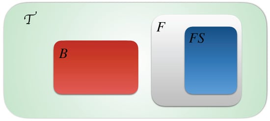
Figure 2.
Distribution of timed local transitions at any time step t of Definitions 4–9.
Delays of local transitions can now be represented in an automata network thanks to timed local transitions. Note that if all delays of local transitions are set to zero, this is equivalent to an AN without delays (original AN). The way these new local transitions should be used is described as follows.
At any time, each automaton has one and only one local state, forming the global state of the network. Choosing arbitrary ordering between automata identifiers, the set of global states of the network is referred to as with . Given a global state , is the local state of automaton a in ζ, i.e., the a-th coordinate of ζ. We write also ⇔; and for any , ⇔. In this paper, we allow, but do not force, applying parallel transitions in different automata, such in Definition 3, but adding delays in the local transitions and considering concurrency between transitions require further study of the semantics of the model (Definition 10).
Definition 10 (Semantics of timed automata network).
Let be a T-AN and . The set of timed local transitions fired at t is:
The state of at is denoted and defined according to the set of timed local transitions that finished at :
then , such that with and
We note that at any time step t, such that and P the set of ongoing transitions, we have: .
Where synchronous biological regulatory networks have been studied, little has been done on the asynchronous counterpart [31], although there is evidence that most living systems are governed by synchronous and asynchronous updating. According to Harvey and Bossomaier [32], asynchronous systems are biologically more plausible for many phenomena than their synchronous counterpart, and observed global synchronous behavior in nature usually simply arises from the local asynchronous behavior. In this paper, we defend these assumptions, and we consider an asynchronous behavior for each automata, on the one hand, and a synchronous behavior in the global network.
In [20], the authors also propose algorithms to learn the delayed dynamic of systems from time series data. However, they focus only on synchronous dynamics, and changes take only one step to occur. The delays that they consider are in the conditions of the change (body of there rules), which can be at different previous time step, where in our method the conditions, are in the same state, and the delay is in the change (head of there rules). However, the assumptions in the synchronous model that all components could change at the same time and take an equivalent amount of time in changing their expression levels are biologically unrealistic. However, there is seldom enough information to be able to discern the precise order and duration of state transitions. The timed extension of AN that we propose in this paper allows both asynchronous and synchronous behavior by proposing a non-deterministic application of the timed local transitions. Table 1 shows a trajectory of a T-AN when we choose to apply timed local transitions in a synchronous manner.

Table 1.
Example of a trajectory of the T-AN of Example 2 starting from an initial state (at ) to a stable state (at ); with as in Definition 9, and B, F, , , , are computed as defined in Definitions 4–8.
We presented above the semantics of the T-AN that we base our work on to model BRNs from experimental data. Even a few hybrid formalisms already exist, like time Petri nets, hybrid automata, etc., we propose this extension of the AN framework for several reasons. First, AN is a general framework that, although it was mainly used for biological networks [28,33], allows one to represent any kind of dynamical models, and converters to several other representations are available. Indeed, a T-AN is a subclass of timed Petri nets [34]. Finally, the particular form of the timed local transition in the T-AN model allows one to easily represent them in ASP, with one fact per timed local transition, as described in this work [35]. Later, we propose a new approach to resolve the generation problem of T-AN models from time series data.
Taking the following T-AN as an example, we generate a possible trajectory of the network starting from a known initial state.
Example 2.
Let be a timed automata extended with delays from Example 1, such that , , , , .
We give in the following Table 1 an example of a trajectory of the T-AN of Example 2 starting from an initial state until reaching a stable state.
4. Learning Timed Automata Networks
This algorithm takes as input a model expressed as a T-AN, whose set of timed local transitions is empty, and time series data capturing the dynamics of the studied system. Given the influences between the components (or assuming all possible influences if no background knowledge is available), this algorithm generates the timed local transitions that could result in the same changes of the model as the observed ones through the observation data.
Algorithm
In this section, we propose an algorithm to build T-AN from time series data. We assume that the latter data observations are provided as a chronogram of size T, with T the maximum number of time points: the value of each variable is given for each time point , , through a time interval discretization (see Definition 11 below and Example in Figure 3 on page 13).
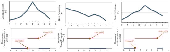
Figure 3.
Examples of the discretization of continuous time series data into bi-valued chronograms. The abscissa (respectively ordinate) represents time (respectively gene expression levels). In this example, the expression level is discretized according to a threshold fixed to half of the maximum gene expression value. change(t) indicates that the expression level of a biological component, here a gene, changes its value at a time point t.
Definition 11 (Chronogram).
A chronogram is a discretization of the time series data for each component of a biological regulatory network. It is presented by the following function Γ,
with T the maximum time point regarding the time series data called the size of the chronogram and n the maximum level of discretization.
We denote a chronogram of the time series data for a component a.
Algorithm 1, MoT-AN (Modeling Timed Automata networks), shows the pseudocode of our implemented algorithm. It will generate all possible timed local transitions that can realize each observed change. A change corresponds to a modification of a component expression level. It happens because of an activation or an inhibition of the changed component by a timed local transition. Thanks to MoT-AN, we compute the discrete levels of the origin and the destination of timed local transitions and the discrete levels of all automata involved in its condition. Thus, finding this timed local transition responsible for this change is also finding the sign of the interaction responsible for this change.
| Algorithm 1 MoT-AN: modeling timed automata networks. |
|
Because of the delays and the non-deterministic semantics, it is not possible to decide whether a timed local transition is absolutely correct or not. However, we can output the minimal sets of timed local transitions, which are necessary to realize all of the dynamics changes. However, since observations are not perfect, we cannot safely remove non-consistent transitions. Thus, we refine the output model by filters taking into account the different possible perturbations. These filters are detailed more later in Section 5.
For the rest of the article, we denote by the last change of each component x comparing to t ( i.e., ).
Theorem 1 (Completeness).
Let be a T-AN, Γ be a chronogram of the components of , i the indegree with and the set of timed local transitions that realized the chronogram Γ, such that . Let χ be the regulation influences of all . Let be a T-AN. Given , Γ, χ and i as input, Algorithm 1 is complete: it will output a set of T-AN ϕ, such that with .
Proof.
Let us suppose that the algorithm is not complete, then there is a timed local transition that realized Γ and . In Algorithm 1, after Step 1, φ contains all timed local transitions that can realize each change of the chronogram Γ. Here, there is no timed local transition that realizes Γ, which is not generated by the algorithm, so . Then, it implies that at Step 2, . However, since h realizes one of the changes of Γ and h is generated at Step 1, then it will be present in one of the minimal subsets of timed local transitions; such that h will be in one of the networks outputted by the algorithm. ☐
If is a T-AN learned model regarding the chronogram Γ and the interaction graph χ of the automata in Σ, such that , which realize .
Theorem 2 (Complexity).
Let be a T-AN, be the number of automata of , η the total number of local states of an automaton of and i the maximal in-degree of all transitions with . Let Γ be a chronogram of the components of over T units of time, such that c is the number of changes in Γ, . The memory use of Algorithm 1 belongs to that is bounded by . The complexity of learning by generating timed local transitions from the observations of Γ with Algorithm 1 belongs to c that is bounded by .
Proof.
Let p be an automaton local state of , then is the maximal number of automaton that can influence p. There is possible combinations of those regulators that can influence p at the same time forming a timed local transition. There is at most T possible delays, so that there are possibles timed local transitions; thus, in Algorithm 1 at Step 1, the memory is bounded by , which belongs to since . Generating all minimal subsets of timed local transitions φ of that can realize Γ can require one to generate at most sets of rules. Thus, the memory of our algorithm belongs to and is bounded by .
The complexity of this algorithm belongs to . Since and , the complexity of Algorithm 1 is bounded by .
Each set has to be compared with the others to keep only the minimal ones, which costs . Furthermore, each set of timed local transitions has to realize each change of Γ; it requires to check that c changes, and it costs . Finally, the total complexity of learning by generating timed local transitions from the observations of Γ belongs to that is bounded by .
In practice, we can fix the maximal indegree of the generated timed local transitions and consider binary automaton (maximum of two local levels per automaton: ) to make the computation tractable. Considering an indegree , the complexity falls down to . If at each time step, there is a change, so it is bounded by .
Indeed, in biological systems, the number of interactions between components is not too large, so it is not the source of complexity, but the fact that we generate all possible minimal models. Besides, behavior can be captured with a simple combination consisting of two components, like in Section 3.2 of [4]. If we output only one model, we find that the complexity falls down to .
5. Refining
In Section 4, we create as many models as possible that satisfy our semantics and the given dynamics (time series data). However, in these models, there may exist some contradictions. Thus, in this section, we introduce a set of refinements to perform model curation and keep the ones that are the most consistent with some given assumptions.
5.1. Synchronous Behavior
As detailed in Section 2, in our semantics, we impose the synchronous semantics behavior as long as there is no conflict between transitions. In other words, for any step, if there is at least one transition τ that is not blocked by another one and τ can be played, then τ should be fired.
Definition 12 (Synchronous and not in conflict transitions).
Let be a learned T-AN model regarding a chronogram Γ and an interaction graph χ of all automata in Σ. The model is said to be coherent with the synchronous and non-conflict behavior in Γ if and only if if is playable at a time step t in Γ and , such that is in conflict with τ, then in Γ with .
This filter checks whether each model is consistent with the synchronous and not in conflict transitions (Theorem 12). If this is not the case, then the model will be discarded from the output of Algorithm 1.
5.2. More Frequent Timed Automata Networks
All outputted models have one execution, which exactly reproduces the given observations (see Theorem 1); thus, it is interesting to compare all of these models and to find the transitions that are more commonly performed.
Definition 13 (Transition frequency).
Let be the set of found models by Algorithm 1. Let be the frequency of appearance of a transition in all of these models:
with,
Giving a minimal frequency to this filter, , it maintains only transitions τ, such that . It can happen that some transitions are lost that are important, but it keeps only the transitions that are more relevant.
5.3. Deterministic Influence
In a T-AN model, we do not want a component to inhibit and activate another with the same level of expression because biologically, this is generally not the case. In Definition 14, we say that the component b with a level of expression k cannot be a part of the conditions that activate () and inhibit () a.
Definition 14 (Distinct influence).
Let be a T-AN model, , , with and . If ∧, then with , .
Therefore, this filter eliminates all learned models in which there exists transitions that do not satisfy the deterministic influences between components (Definition 14).
5.4. Several Delays
Usually in the same model for the same transition, there is only one delay. However, when learning models from real-time series data (e.g., data coming from cell cancer lineages, circadian clock, …), we may not be guaranteed that the data have been normalized, even after discretization. Indeed, there is often noise in data. Thus, after computing the delays, Algorithm 1 can find the same transition with different delays. Here, the user (biologist) can choose whether to keep all of these transitions or we propose to him/her to merge all of them and keep only one transition with an interval of delays by computing the maximum value and the minimum one.
Definition 15 (Interval of delays).
t.q , , ..., with , and then: merge all transitions in one transition τ:
such that:
On the other hand, we can compute a delay equal to the average value of all of these transitions that differ only by delays (see Definition 16). The intuition is that, in practice, if there are enough observations, the delay of those actions should tend to the real value.
Definition 16 (Average of delays).
t.q , , ..., with , and then: merge all transitions in one transition τ:
such that:
In Definition 17, we want each learned transition to have only one delay in one model.
Definition 17 (deterministic delay)
Let be a T-AN model, if such that , , , then .
6. Case Study
In this section, we show how this method generates a T-AN model consistent with the set of biological regulatory time series data. First, the method uses discretized observations as an input (i.e., chronogram), thus, it is necessary to process at the beginning the time series data with another method (as shown in Figure 3) in order to discretize it.
Our method may be summarized as follows:
- -
- Detect biological components’ changes;
- -
- Compute the candidate timed local transitions responsible for the network changes;
- -
- Generate the minimal subset of candidate timed local transitions that can realize all changes;
- -
- Filter the timed candidate actions.
We apply Algorithm 1 on learning the timed local transition of the example of a network with 3 components () whose chronogram is detailed in Figure 3 on page 13:
The first change occurs at , denoted by . It is the gene z whose value changes from zero to one; thus the timed local transition that has realized this change has this form , where ℓ can be any combination of the values of the regulators of z.
Let be the set of regulation influences among the components of the network. According to χ, the set of genes having influence on z is . This means that , or , or . The expression level of the genes of when the researched candidate timed local transition () is ongoing, i.e., during the partial steady state between two successive changes ( and ). This level is computed from the chronograms as follows:
Thus, ℓ= or ℓ= or ℓ=, and the set of candidate timed local transitions is: . Since it is the first change, the delay of each timed local transition is the same: .
The second change occurs at and is denoted by . Here, it is the gene a whose state changes from to ; thus, the timed local transition that realizes this change has this form where ℓ can be any combination of the regulators value at of z. According to χ, the genes influencing a are . This means that , and the expression level of a between and is . Therefore, . Thus, there is only one candidate timed local transition: .
The third change occurs at , . Here, it is the gene b whose value changes from to ; thus, the timed local transition that realizes this change is of this form, where ℓ can be any combination of the regulators value at of b. According to χ, there is no gene that can influence b; thus, no timed local transition can realize this change.
The fourth change occurs at , . Here, it is a whose expression decreases and changes from to ; thus, the candidate timed local transition that could realize this change has this form, where ℓ can be any combination of the regulators value at of a. According to χ, the set of genes having influences on a is . Again, as the expression level of a since its last change is . We have , and there is only one candidate timed local transition: .
The fifth change occurs at , . Here, it is z whose value changes from to ; thus, the time local transition that has realized this change has the form of: where ℓ can be any combination of the regulators’ value at of b. Since , this means that or or The expression level of a and b at is respectively and . Thus, or or . The candidate timed local states are:
The last change of a is at , and the last change of b is at . Thus, , , .
After processing all changes, the set of timed local transitions that could realize the chronograms is:
All learned timed local transitions are consistent with all observed time series data and the regulation influences given as input. The used method ensures completeness; we have the full set of timed local transitions that can explain the observations. By generating all minimal subsets of this set of timed local transitions, one of those subsets (as in Figure 4) define the model that realized the observations.
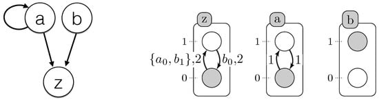
Figure 4.
(Left) Influence graph modeling of the case study example (Figure 3); (right) one of the T-AN generated by Algorithm 1. The labels of each local transition stand for the local states of the automata, which make the transition playable, and its delay (time needed for the transition to be performed).
7. ASP Encoding
7.1. ASP Syntax
In this section, we briefly recapitulate the basic elements of ASP [36], a declarative language that proved efficient to address highly computational problems. An answer set program is a finite set of rules of the form:
where , is a propositional atom or ⊥; all are propositional atoms, and the symbol “” denotes negation as failure. The intuitive reading of such a rule is that whenever are known to be true and there is no evidence for any of the negated atoms to be true, then has to be true, as well. If , then the rule becomes a constraint (in which case the symbol ⊥ is usually omitted). As ⊥ can never become true, if the right-hand side of a constraint is validated, it invalidates the whole solution.
In the ASP paradigm, the search of solutions consists of computing the answer sets of a given program. An answer set for a program is defined by Gelfond and Lifschitz [37] as follows. An interpretation I is a finite set of propositional atoms. A rule r as given in (1) is true under I if and only if:
An interpretation I is a model of a program P if each rule is true under I. Finally, I is an answer set of P if I is a minimal (in terms of inclusion) model of , where is defined as the program that results from P by deleting all rules that contain a negated atom that appears in I and deleting all negated atoms from the remaining rules. Programs can yield no answer set, one answer set or several answer sets. To compute the answer sets of a given program, one needs a grounder (to remove free variables from the rules) and a solver. For the present work, we used CLINGO(we used CLINGO Version 5.0: http://potassco.sourceforge.net/) [38], which is a combination of both.
In the rest of this section, we use ASP to tackle the problems’ learning models from the time series data (i.e., implementing Algorithm 1 and all of the refinements in Section 5).
7.2. All Models
Encoding of the case study in Section 6, Figure 3 on page 13: We encode the observations as a set of predicates obs(X,Val,T), where X is an automaton identifier, Val a level of this automaton and T is a time point, such that the automaton X has the value Val starting from T.
1 % All network components with its levels after discretization
2 automatonLevel("a",0..1). automatonLevel("b",0..1). automatonLevel("c",0..1).
3 % Time series data or the observation of the components
4 obs("a",0,0). obs("a",0,1). obs("a",0,2). obs("a",0,3). obs("a",1,3). obs("a",1,4). obs("a",1,4).
5 obs("a",1,5). obs("a",0,5). obs("a",0,6). obs("a",0,7). obs("b",1,0). obs("b",1,1). obs("b",1,2).
6 obs("b",1,3). obs("b",1,4). obs("b",0,4). obs("b",0,5). obs("b",0,5). obs("b",0,6). obs("b",0,7).
7 obs("c",0,0). obs("c",0,1). obs("c",0,2). obs("c",1,2). obs("c",1,3). obs("c",1,4). obs("c",1,5).
8 obs("c",1,6). obs("c",0,6). obs("c",0,7).
We define in the predicate changeState(X,Val1, Val2, T), the time point T where X changes its level from Val1 to Val2. We admit that at t=0, all components change (lines 11–12). Then, to reduce the complexity of the program, we consider in the predicate time only the time points where the components change their levels (line 18). Similar for the delays, D is a delay when it is equal to the difference between two time steps where some components change their levels (line 19). To compute the chronogram of a component a, we compute the time points where it is constant (i.e., has only one level) between two successive changes of a: T1 and T2 (lines 21–22).
 9 % Changes identification
10 % initialization of all changes for each automaton at t=0 (assumption)
11 changeState(X,Val,Val,0) ← obs(X,Val,0).
12 changeState(X,0) ← obs(X,_,0).
13 % Compute all changes of each component according to the observations (chronogram)
14 changeState(X,Val1, Val2, T) ← obs(X, Val1, T), obs(X,Val2,T),obs(X, Val1, T-1), obs(X, Val2, T+1),
15         Val1!=Val2.
16 changeState(X,T) ← changeState(X,_,_,T).
17 % Find all time points where changes occure (reduce complexity)
18 time(T) ← changeState(_,T).
19 delay(D) ← time(T1), time(T2), D=T2-T1, T2>=T1.
20 % Observations processing
21 obs_normalized(X,Val,T1,T2) ← obs(X,Val,T1), obs(X,Val,T2), T1<T2, not existChange(X,Val,T1,T2),
22         time(T1), time(T2).
23 % Verify if X changes its level between two time points T1 and T2
24 existChange(X,Val,T1,T2) ← obs(X,Val,T1), obs(X,Val,T2), obs(X,Val1,T), T>T1, T<T2, Val!=Val1.
25 existChange(X,Val,T1,T2) ← obs(X,Val,T1), obs(X,Val,T2), changeState(X,T), T>T1, T<T2.
26 existChange(X,Val,T1,T2) ← obs(X,Val,T1), obs(X,Val,T2), T1<T2, changeState(X,Val,Val_,T1), Val!=Val_.
We detailed in Section 3 how to compute the delays. Therefore, the delay is the difference between the time where the change happens (changeState) and the last change of the components involved in the local transition: the influenced one, X, and the influencing one(s) (here, we detail only the transition with indegree = 1). Find the last component that has changed, the influenced component X, the influencing component Y or one of the components influenced by X, such that there exists a transition in conflict with the computing one. This last time step of the change H comparing to the time step T2 for the component X having as an influence Y is computed in the predicate lastChange(X,Y,H,T2) (lines 29–39). In other words, H=
.
27 % Find the time step when the transition has started playing
28 % The last change of X such that W is influencing by X and X is influencing by Y
29 lastchange(X,Y,W,Max,T2) ← Max=#max{ T : changeState(Y,T;X,T;W,T), T<T2}, changeState(X, T2),
30         existInfluence(X,Y), existInfluence(W,X), Max>=0.
31 lastChangeAll(X,Y,Max,T2) ← lastchange(X,Y,W,Max,T2), transition(X,_,W,_,_,D, change(T3)), T3<T2,
32         T2-U>D, lastConditionChange(X,Y,U,T2).
33 % Last change between X and its influencing component Y
34 lastConditionChange(X,Y,H,T2) ← H=#max{ T : changeState(Y,T;X,T) , T<T2}, changeState(X, T2),
35         existInfluence(X,Y), H>=0.
36 % Find the time point of the  last change: it is the last change of X, or of the component influenced by X
37 % or of the components involved in the transition condition
38 lastChange(X,Y,Max,T2) ← lastChangeAll(X,Y,Max,T2).
39 lastChange(X,Y,H,T2) ← lastConditionChange(X,Y,H,T2), not lastChangeAll(X,Y,H,T2), H!=H, delay(H).
We propose below Figure 5 where we simplify the explication of the encoding part. It illustrates which resources are necessary to compute the origin, destination, conditions and delay of each timed local transition.
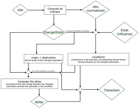
Figure 5.
An illustration of how the ASP encoding computes the timed local transitions "transition" from the observations "obs". The names in lozenges correspond to the predicates in the ASP code.
To create as many models as possible that satisfy the given time series data, we add in the head of the rule the brackets { } between the predicates of the transition (see lines 41–43). Then, we make sure that we keep exactly one transition for each change at a step T by component X. We compute this number of different transitions in Tot by the predicate getTransNumber(Tot,X,T) (line 46). Therefore, we eliminate all models that do not satisfy this assumption by the constraints in lines 48–49.
40 % Compute all models with all candidate timed local transitions
41 {transition(Y,Valy,X,Val1,Val2,D, change(T2))} ← obs_normalized(X,Val1,T1,T2),
42         obs_normalized(Y,Valy,T1,T2), changeState(X,Val1,Val2,T2), existInfluence(X,Y),
43         lastChange(X,Y,T1,T2), T2=T1+D, delay(D).
44 transition(Y,Valy,X,Val1,Val2,D) ← transition(Y,Valy,X,Val1,Val2,D, _).
45 % for each change keep only one transition (xOR)
46 getTransNumber(Tot,X,T)← Tot={transition(_,_,X,_,_,_, change(T))}, changeState(X,T), T!=0.
47 % Exactly one transition by change in a model
48 ← getTransNumber(Tot,X,T), changeState(X,T), Tot=0.
49 ← getTransNumber(Tot,X,T), changeState(X,T), Tot>1.
7.3. Refinement
In this section, we show the encoding part of the filters presented in Section 5 to eliminate all contradiction between transitions in the same model or between the transition and the semantics.
7.4. Refinement According to the Semantics
The following constraint ensures that each output model will respect Definition 14: a component cannot inhibit and activate another one with the same level (line 51).
50 % A component with the same level inhibits and activates the same component
51 ← transition(Y,Valy,X,Val1,Val2,_), transition(Y,Valy,X,Val3,Val4,_), Val1<Val2, Val3>Val4.
Furthermore, according to Definition 14, a component cannot have the same effect on another one with the same level of expression. This property is encoded by the following constraint (line 53).
52 % A component with different levels influence another component with the same effect
53 ← transition(Y,Valy,X,Val1,Val2,_), transition(Y,Valy_,X,Val1,Val2,_), Valy_!=Valy.
According to Definition 12, a transition that is playable at a time point and that is not in conflict with another one should be played (synchronous behavior). If this is not the case, the model is not correct and will be eliminated by the following constraint in lines 68–69.
54 % Last time points in the data
55 timeSeriesSize(Last) ← Last=#max{ T : obs(_,_,T) }.
56 step(0..Last)← timeSeriesSize(Last).
57 % Compute all the obs between all the time points in the data
58 obs_(X,Val,T1,T2) ← obs(X,Val,T1), obs(X,Val,T2), T1<T2, not existsChange(X,Val,T1,T2).
59 existsChange(X,Val,T1,T2) ← obs(X,Val1,T), T>T1, T<T2, Val1!=Val, obs(X,Val,T1), obs(X,Val,T2).
60 % There is a transition with different delays
61 existTransDiffDelays(Y,Valy,X,Val1,Val2,D1,D2) ← transition(Y,Valy,X,Val1,Val2,D1),
62         transition(Y,Valy,X,Val1,Val2,D2), D1!=D2.
63 % There is a transition in conflict with "transition(Y,Valy,X,Val1,Val2,D1)"
64 existTransInConflict(Y,Valy,X,Val1,Val2,D1,T1,T2) ← transition(Y,Valy,X,Val1,Val2,D1),
65         transition(X,Val1,_,_,_,D2,change(T3)), T3>=T2, D2>=D1, T3-D2 <=T2, step(T2),
66         step(T1), T1<T2, D1=T2-T1, obs_(X,Val1,T1,T2), obs_(Y,Valy,T1,T2).
67 % Eliminate all models that do not respect the semantics (Definitions 5–6)
68 ← transition(Y,Valy,X,Val1,Val2,D), obs_(X,Val1,T1,T2), obs_(Y,Valy,T1,T2), step(D),
69         not changeState(X,Val1,Val2,T2), not existTransInConflict(Y,Valy,X,Val1,Val2,D,T1,T2),
70         not existTransDiffDelays(Y,Valy,X,Val1,Val2,D,D2), changeState(X,Val1,Val2,T3),
71         T2!=Max, timeSeriesSize(Max), obs_(X,Val1,T1,T3), T3-T1=D2, delay(D2), D=T2-T1.
7.5. Refinement on the Delays
The several refinements of the generated models we propose can be seen as parameters that can be combined or not. For example, the user can specify that for the same transition, if we find different delays, we can take the average value or even specify an interval in which we define the minimum value and the maximum value.
According to Definition 17, in one model, a transition cannot have different delays; so that such models can be eliminated by the following constraint in line 12.
73 % No different delays for the same transition
74 ← transition(Y,Valy,X,Val1,Val2,D1), transition(Y,Valy,X,Val1,Val2,D2), D1!=D2.
Otherwise, we can merge all transitions that only differ by their delay in one transition, but whose delay is equal to the average delay of these transitions. To compute the average delays for a transition in the same model according to Definition 16, we do as follows in ASP. First, we compute the total number of these transitions in Tot by nbreTotTrans(Y,Valy,X,Val1,Val2,Tot) (lines 77–77), where the shared part between all transitions is Y,Valy,X,Val1,Val2; then, the sum of all of these delays in S by the predicate sumDelays (lines 80–81). To find the average, we divide S by Tot (Davg=S/Tot). The new transition after merging is then transAvgDelay(Y,Valy,X,Val1,Val2,Davg) (lines 83–84).
75 % Transitions with the average of delays
76 % Number of the repetition of each transition
77 nbreTotTrans(Y,Valy,X,Val1,Val2,Tot) ← Tot={transition(Y,Valy,X,Val1,Val2,_,_)},
78         transition(Y,Valy,X,Val1,Val2,_).
79 % The sum of the delays for each transition
80 sumDelays(Y,Valy,X,Val1,Val2,S) ← S=#sum{ D: transition(Y,Valy,X,Val1,Val2,D)},
81         transition(Y,Valy,X,Val1,Val2,_), S!=0.
82 % Compute the average delay for each transition
83 transAvgDelay(Y,Valy,X,Val1,Val2,Davg) ← nbreTotTrans(Y,Valy,X,Val1,Val2,Tot),
84 sumDelays(Y,Valy,X,Val1,Val2,S), Davg=S/Tot.
It is also possible to compute the interval of the delays according to Definition 15: [Max, Min] with Max is the maximum value of the delays of this transition, computed by the predicate maxDelay (lines 86–87); Min is the minimum value of the delays computed by the predicate minDelay (lines 88–89). Finally, the generation of a transition after merging is done by the predicate transIntervalDelay in lines 90–91.
85 % Compute the maximum value and the minimum value of the delays of a same transition
86 maxDelay(Y,Valy,X,Val1,Val2,Max) ← Max=#max{ D : transition(Y,Valy,X,Val1,Val2,D)},
87         transition(Y,Valy,X,Val1,Val2,_).
88 minDelay(Y,Valy,X,Val1,Val2,Min) ← Min=#min{ D : transition(Y,Valy,X,Val1,Val2,D)},
89         transition(Y,Valy,X,Val1,Val2,_).
90 transIntervalDelay(Y,Valy,X,Val1,Val2,interval(Min,Max)) ← minDelay(Y,Valy,X,Val1,Val2,Min),
91         maxDelay(Y,Valy,X,Val1,Val2,Max).
According to the Definition 13, we want to find the more frequent transitions in the models. In ASP, the option "
” computes the cautious consequences (intersection of all answer sets) of a logic program (algorithm implementation in ASP). Therefore, we use this option while executing.
8. Evaluation
In this section, we provide two assessments of Algorithm 1. We evaluate the capacity of our algorithm ( all programs, described in this article for timed automata network generation are implemented in ASP and are available online at: http://www.irccyn.ec-nantes.fr/~benabdal/modeling-biological-regulatory-networks.zip) to build models for prediction and the impact of the quantity of observations on run time. Here, we process chronograms obtained from time series data of the DREAM4 challenge [39] and of the DREAM8 challenge [40].
8.1. DREAM4
In this section, we assess the efficiency of our algorithm through case studies coming from the DREAM4 challenge. DREAM challenges are annual reverse engineering challenges that provide biological case studies. In this section, we focus on the datasets coming from DREAM4 (available online at https://www.synapse.org/#!Synapse:syn3049712/wiki/74630). It provides data for systems of different size (10 genes on the one hand; 100 genes on the other), allowing us to assess the scalability of our approach. The input data that we tackle here consist of the following: five different systems each composed of 100 genes, all coming from Escherichia coli and yeast networks. For every such system, the available data are the following: (i) 10 time series data with 21 time points, and 1000 is the duration of each time series; (ii) steady state for the wild-type; (iii) steady states after knocking out each gene; (iv) steady states after knocking down each gene (i.e., forcing its transcription rate at 50%); (v) steady states after some random multifactorial perturbations. We processed all of the data. Here, we focus on the management of time series data.
Each time series includes different perturbations that are maintained all of the time during the first 10 time points and applied to at most 30% of the genes. In this setting, a perturbation means a significant increase or decrease of the gene expression. In the raw data of the time series, gene expression values are given as real numbers between zero and one.
The discretization is a crucial part for the abstraction of the data. However, in this article, we do not develop the method of the discretization, and we suppose this as already chosen. There are many ways to discretize those data; using biological databases and statistical methods, we could identify gene expression thresholds. Clustering techniques could be used to group data points into discrete levels. On the other hand, rather than considering thresholds, we could focus on components’ speed evolution to discretize the data. It is indeed a perspective of optimization to regularize the model through different levels and methods of discretization. However, in this article, we focus on the learning algorithm and consider discretization as more or less given.
To apply our approach, we chose to discretize those data into two to six qualitative values. Increasing the number of qualitative values from two to four improves the precision, but then the score decreases from five, most likely because of over-fitting: the relations learned become too precise and cannot be applied on something else other than the training data. The best score we obtained was with four qualitative values and is reported in Table 2. Each gene is discretized in an independent manner, with respect to the following procedure: we compute the average value of the gene expression among all data of a time series, then the values between the average and the maximal/minimal value are divided into as many levels. Discretizing the data according to the average value of expression is expected to reduce the impact of perturbation on the discretization and, thus, on the model learned.
Table 2.
Evaluation of our method on the learning and prediction of the evolution of gene regulatory network benchmarks from the DREAM4 challenge [39] through the Mean Square Error (MSE): 10 variables benchmarks (left); and 100 variables benchmarks (right).
The DREAM4 challenge offers two different problems, which consist of predicting: (i) the structure of the gene interactions (in terms of an unsigned directed graph); (ii) attractors in some given conditions. Our method is not designed to tackle the first issue; indeed, we need to know those influences. However, the models we learn can be applied to predict trajectories and thus attractors. Here, we use the influences graphs expected in the first problem as the background knowledge (inferred by the Gene Network Weaver [41]) to tackle the attractor prediction part of the challenge.
8.2. Results
For this evaluation, we are given an initial state and five different dual gene knockout conditions. The goal is to predict the attractor in which the system will fall from the initial state for each dual knockout. Here, we just choose the first model that our algorithm outputs and use the biggest set of fireable timed local transitions at each time step to produce a trajectory until a cycle is detected. The first state of this cycle is reverse discretized and proposed as the predicted state. In the challenge, the quality of the prediction is evaluated by computing the mean square error (MSE) between the predicted state and the expected one. As shown in Table 2, the precision we achieved in those experiments is quite good considering the results of the competitors of the DREAM4 challenge [39]. Their results range between 0.010 and 0.075 for the same evaluation settings, which are comparable to (0.033 to 0.086), giving us encouraging results. Regarding run time, learning and predicting the trajectories of the benchmarks of 10 genes took less than 30 s, and the same experiments for the benchmarks of 100 genes took about 3 h and 20 min on a one-processor Intel Core2 Duo (P8400, 2.26 GHz).
To achieve this score, we had to perform several tests by varying the discretization precision and the complexity of the dynamics learned. Figure 6 shows the score we got on predicting the training data of DREAM4 benchmarks of size 10 starting with two levels of discretization until 20. Here, we take the series of each benchmark as the input, and the first state of each series is used to start a prediction. MSE is computed over the 21 points of the original series against the predicted ones. We can see that increasing the discretization precision improves the prediction precision until five levels of discretization. Then, the model prediction quality decreases as it tends to overfit the data. Those tests also allow us to assess the scalability of our approach in practice. Figure 7 shows the impact of both timed local transition indegree and discretization level on run time when learning the DREAM4 benchmarks of size 100.
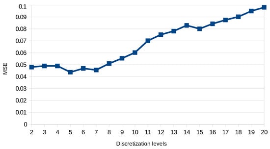
Figure 6.
Evaluation of the discretization impact on model precision over training data of DREAM4 benchmarks of a size of 10.
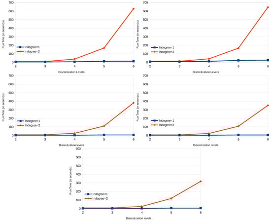
Figure 7.
Evolution of run time on processing different models inferred from time series data of DREAM4 (100 variables benchmarks), varying the indegree of local timed transitions and discretization levels. These tests were performed on a processor of Intel Core i7 (4700, 3 GHz) with 16 GB of RAM.
In the results obtained from the experimentation of our algorithm on the time series data of the DREAM4, we can see the exponential influence on the run time of the indegree per local transition considered, as well as the level of discretization chosen for all five different networks. However, it also shows that in practice, our approach can tackle big networks; here, 100 genes.
8.3. DREAM8
We recently started to test our method on the DREAM8 [40]: Heritage-DREAM breast cancer network inference challenge (the data set is available online at https://www.synapse.org/#!Synapse:syn1720047/wiki/55342). The challenge is about the inference of causal signaling networks and prediction of protein phosphorylation dynamics. As for DREAM4, we are focusing on the prediction part. The aim is to build dynamical models that can predict trajectories of phosphoproteins. An important emphasis is on the ability of models to generalize beyond the training data by predicting trajectories under perturbations not seen in the training data. This sub-challenge is split into two independent parts: A, breast cancer proteomic data; B, in silico data; and we choose to start with the first one.
Training data come from experiments on four breast cancer cell lines stimulated with various ligands. The data comprise protein abundance time courses under inhibitor perturbations. Training data are provided for each of the 32 biological contexts defined by the combination of cell line and growth condition (stimulus). These data comprise time courses for about 45 phosphoproteins under a vehicle control (DMSO) and under inhibitor perturbations of network nodes, as shown in Figure 8 (Figure 8 is from https://www.synapse.org/#!Synapse:syn1720047/wiki/56061). Using these training data, participants are asked to build dynamical models that can predict phosphoprotein trajectories specific to each of the 32 biological contexts (32 cell line/stimulus pairs) and under the inhibition of phosphoproteins that were not perturbed in the training data.
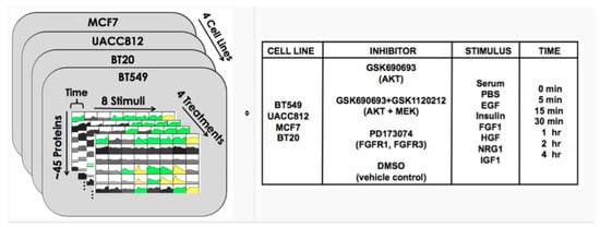
Figure 8.
DREAM8 time series data [42].
Here, we deal with about 48 variables per cell line, which is tractable for our algorithm. The quantity of time series is also more generous than in DREAM4. The difficulty for us lies in the small amount of data point per series: seven points (0, 5, 15, 30, 60 min and 2, 4 h). Even though, we succeed at producing models that can be used for the time course prediction.
8.4. Results
To evaluate their precision, predicted trajectories are compared with experimental test data obtained in each of the 32 cell line/stimulus contexts and following the inhibition of phosphoprotein nodes by test inhibitors. These experiments are over the same time period as the training data (up to 4 h). To get our precision score, we used dreamtools [43], an open-source Python package for evaluating DREAM challenge scoring metrics. The scoring metric of this sub-challenge is based on multiple metrics; so far, we focused on the mean RMSE (Root Mean Squared Error) provided by dreamtools. In those experiments, we chose to abstract the data into a fixed number of discrete levels as for the DREAM4 experiment (see Section 8.1). By varying the number of level of discretization (see Table 3), our best score was obtained with five levels of discretization. Considering less levels results in a prediction that is too general, while considering more levels results in a tendency to overfit the modelw.r.t. the observed data. The best score we could get so far was 0.5528 mean RMSE, which would rank our method around the ninth and 11th leader board method (the DREAM8 Subchallenge 2A leader board is available at https://www.synapse.org/#!Synapse:syn1720047/wiki/56831), which got scored between 0.5139 and 0.5564 on this metric. On this challenge, the best performing methods are based on statistical analysis (see https://www.synapse.org//#!Synapse:syn2343141). The interest of our method is that the model we learn is human readable, as well as the trajectory prediction. Indeed, we explain the dynamical behavior of the network by providing detailed interactions between components to explain each change step by step. These transitions are enriched by signs (activation/inhibition), the level of expression (thresholds) and delays. The final model can be understood statically and can be used to predict dynamical behaviors with respect to a known semantics.
Table 3.
Evaluation results of our methods on DREAM8 Subchallenge 2A data.
Like for DREAM4, to achieve this score, we had to perform several tests by varying the discretization precision and the complexity of the dynamics learned. Table 4 shows the score we got on predicting the training data of DREAM8 benchmarks with two and five levels of discretizations (here, we show only the detailed score for two levels, because of time (about 15 h per level after five)).
Table 4.
Evaluation results of our methods on DREAM8 training data.
8.5. Discussion
We propose a new method, MoT-AN (Algorithm 1), to automatically infer models that could explain the dynamical evolution of the biological systems. The contribution of our method lies in the fact that it identifies the set of interactions between biological components by concertizing the signs (negative or positive), providing thresholds and associating the quantitative time delays for each local transition.
We illustrated the merits of this method by applying it on large real biological systems (DREAM4 and DREAM8 challenges). As a result, we obtain in a few seconds models that are proven to be relevant (this relevance is qualified in terms of mean square error using dream tools) This algorithm is implemented using ASP [36,44], thus providing the exhaustive enumeration of all models.
The main limit of the approach presented in this paper is the fact that the topology of the network is considered as granted. As discussed in the Introduction of the paper, there is a wide range of algorithms designed to address this issue [41,45]. Furthermore, such interaction graphs could be deduced from the available reliable databases of biological networks. Some examples of databases for human regulatory knowledge are: the Pathways Interaction Database [46], the Human Integrated Pathway DB [47] and the Causal Biological Network Database [48].
Various inference approaches [46,49,50] from time series data based on prior knowledge about component interactions have been proposed. However, they share a common limit: they focus on static characterization of the interactions, and they do not allow one to infer dynamic behaviors where delays are involved. The merits of our contribution lie in the fact that we overcome such limits, and we infer delays in a qualitative dynamic modeling of the network.
9. Conclusions and Perspectives
In this paper, we propose an approach that takes the background knowledge under the form of regulation graph and time series data as the input. The originality of our work is three-fold: (i) the identification of the sign of the interactions; (ii) the direct integration of quantitative time delays in the learning approach; and (iii) the identification of the qualitative discrete levels that lead to the systems dynamics. As a result, we produce a set of T-AN that explains the biological network evolution. Algorithm 1 is implemented in ASP. We illustrated the applicability and limits of the proposed method through benchmarks from DREAM4. We also improved our method and made it more robust against noisy and scarce data by proposing some refinements. Then, we applied it on the DREAM8 dataset: Heritage-DREAM breast cancer network. These results open the way to promising applications in the cooperation between biologists and computer scientists. Further works now consist of discussing the kind of information one can get on T-AN by analyzing the associated non-timed model.
Supplementary Materials
The supplementary materials are available online at www.mdpi.com/1999-4893/10/1/8/s1.
Acknowledgments
We thank Laurent Trilling for valuable discussions.
Author Contributions
Emna Ben Abdallah and Tony Ribeiro did the formalization. Emna Ben Abdallah designed and implemented the algorithms. Tony Ribeiro performed the experiments. Emna Ben Abdallah and Tony Ribeiro wrote the paper. Morgan Magnin and Olivier Roux and Katsumi Inoue supervised the work.
Conflicts of Interest
The authors declare no conflict of interest.
Abbreviations
The following abbreviations are used in this manuscript:
| AN | Automata Network |
| T-AN | Timed Automata Network |
| ASP | Answer Set Programming |
References
- Marx, V. Biology: The big challenges of big data. Nature 2013, 498, 255–260. [Google Scholar] [CrossRef] [PubMed]
- Callebaut, W. Scientific perspectivism: A philosopher of science’s response to the challenge of big data biology. Stud. Hist. Philos. Sci. Part C 2012, 43, 69–80. [Google Scholar] [CrossRef] [PubMed]
- Fan, J.; Han, F.; Liu, H. Challenges of big data analysis. Natl. Sci. Rev. 2014, 1, 293–314. [Google Scholar] [CrossRef] [PubMed]
- Akutsu, T.; Kuhara, S.; Maruyama, O.; Miyano, S. Identification of genetic networks by strategic gene disruptions and gene overexpressions under a Boolean model. Theor. Comput. Sci. 2003, 298, 235–251. [Google Scholar] [CrossRef]
- Sima, C.; Hua, J.; Jung, S. Inference of gene regulatory networks using time-series data: A survey. Curr. Genom. 2009, 10, 416–429. [Google Scholar] [CrossRef] [PubMed]
- Koksal, A.S.; Pu, Y.; Srivastava, S.; Bodik, R.; Fisher, J.; Piterman, N. Synthesis of biological models from mutation experiments. In Proceedings of the 40th Annual ACM SIGPLAN-SIGACT Symposium on Principles of Programming Languages, Rome, Italy, 23–25 January 2013; Volume 48, pp. 469–482.
- Kim, S.Y.; Imoto, S.; Miyano, S. Inferring gene networks from time series microarray data using dynamic Bayesian networks. Brief. Bioinform. 2003, 4, 228–235. [Google Scholar] [CrossRef] [PubMed]
- Zhao, W.; Serpedin, E.; Dougherty, E.R. Inferring gene regulatory networks from time series data using the minimum description length principle. Bioinformatics 2006, 22, 2129–2135. [Google Scholar] [CrossRef] [PubMed]
- Koh, C.; Wu, F.X.; Selvaraj, G.; Kusalik, A.J. Using a state-space model and location analysis to infer time-delayed regulatory networks. EURASIP J. Bioinform. Syst. Biol. 2009, 2009. [Google Scholar] [CrossRef] [PubMed]
- Liu, T.F.; Sung, W.K.; Mittal, A. Learning multi-time delay gene network using Bayesian network framework. In Proceedings of the 16th IEEE International Conference on Tools with Artificial Intelligence, Boca Raton, FL, USA, 15–17 November 2004; pp. 640–645.
- Silvescu, A.; Honavar, V. Temporal Boolean network models of genetic networks and their inference from gene expression time series. Complex Syst. 2001, 13, 61–78. [Google Scholar]
- Zhang, Z.Y.; Horimoto, K.; Liu, Z. Time Series Segmentation for Gene Regulatory Process with Time-Window-Extension. In Proceedings of the 2nd International Symposium on Optimization and Systems Biology, Lijiang, China, 31 October–3 November 2008; pp. 198–203.
- Akutsu, T.; Tamura, T.; Horimoto, K. Completing networks using observed data. In Algorithmic Learning Theory; Springer: Berlin/Heidelberg, Germany, 2009; pp. 126–140. [Google Scholar]
- Matsuno, H.; Doi, A.; Nagasaki, M.; Miyano, S. Hybrid Petri net representation of gene regulatory network. Pac. Symp. Biocomput. 2000, 5, 341–352. [Google Scholar]
- Siebert, H.; Bockmayr, A. Temporal constraints in the logical analysis of regulatory networks. Theor. Comput. Sci. 2008, 391, 258–275. [Google Scholar] [CrossRef]
- Ahmad, J.; Bernot, G.; Comet, J.P.; Lime, D.; Roux, O. Hybrid modelling and dynamical analysis of gene regulatory networks with delays. ComPlexUs 2006, 3, 231–251. [Google Scholar] [CrossRef]
- Casagrande, A.; Dreossi, T.; Piazza, C. Hybrid Automata and epsilon-Analysis on a Neural Oscillator. In Hybrid Systems Biology: First International Workshop, HSB 2012, Newcastle Upon Tyne, UK; Cinquemani, E., Donzé, A., Eds.; Lecture Notes in Computer Science; Springer International Publishing: Cham, Switzerland, 2012; pp. 58–72. [Google Scholar]
- Paoletti, N.; Yordanov, B.; Hamadi, Y.; Wintersteiger, C.M.; Kugler, H. Analyzing and synthesizing genomic logic functions. In Computer Aided Verification; Springer: Cham, Switzerland, 2014; pp. 343–357. [Google Scholar]
- Li, R.; Yang, M.; Chu, T. Synchronization of Boolean networks with time delays. Appl. Math. Comput. 2012, 219, 917–927. [Google Scholar] [CrossRef]
- Ribeiro, T.; Magnin, M.; Inoue, K.; Sakama, C. Learning delayed influences of biological systems. Front. Bioeng. Biotechnol. 2014, 2. [Google Scholar] [CrossRef] [PubMed]
- Donnarumma, F.; Murano, A.; Prevete, R.; della Battaglia, V.S.M. Dynamic network functional comparison via approximate-bisimulation. Control Cybern. 2015, 44, 99–127. [Google Scholar]
- Girard, A.; Pappas, G.J. Approximate bisimulations for nonlinear dynamical systems. In Proceedings of the 44th IEEE Conference on Decision and Control and European Control Conference (CDC-ECC 2005), Seville, Spain, 12–15 December 2005; pp. 684–689.
- Comet, J.P.; Fromentin, J.; Bernot, G.; Roux, O. A formal model for gene regulatory networks with time delays. In Computational Systems-Biology and Bioinformatics; Springer: New York, NY, USA, 2010; pp. 1–13. [Google Scholar]
- Merelli, E.; Rucco, M.; Sloot, P.; Tesei, L. Topological characterization of complex systems: Using persistent entropy. Entropy 2015, 17, 6872–6892. [Google Scholar] [CrossRef]
- Merelli, E.; Pettini, M.; Rasetti, M. Topology driven modeling: The IS metaphor. Nat. Comput. 2015, 14, 421–430. [Google Scholar] [CrossRef] [PubMed]
- Ben Abdallah, E.; Ribeiro, T.; Magnin, M.; Roux, O.; Inoue, K. Inference of Delayed Biological Regulatory Networks from Time Series Data. In Computational Methods in Systems Biology, Proceedings of the 14th International Conference, CMSB, Cambridge, UK, 21–23 September 2016; Springer International Publishing AG: Dordrecht, The Netherlands, 2016; pp. 30–48. [Google Scholar]
- Paulevé, L.; Magnin, M.; Roux, O. Refining Dynamics of Gene Regulatory Networks in a Stochastic π-Calculus Framework. In Transactions on Computational Systems Biology XIII; Springer: Berlin/Heidelberg, Germany, 2011; Volume 6575, pp. 171–191. [Google Scholar]
- Paulevé, L.; Chancellor, C.; Folschette, M.; Magnin, M.; Roux, O. Analyzing Large Network Dynamics with Process Hitting. In Logical Modeling of Biological Systems; Wiley: New York, NY, USA, 2014; pp. 125–166. [Google Scholar]
- Paulevé, L. Goal-Oriented Reduction of Automata Networks. In Computational Methods in Systems Biology Proceedings of the 14th International Conference, CMSB, Cambridge, UK, 21–23 September 2016; Springer International Publishing AG: Dordrecht, The Netherlands, 2016. [Google Scholar]
- Goldstein, Y.A.; Bockmayr, A. A lattice-theoretic framework for metabolic pathway analysis. In Computational Methods in Systems Biology; Springer: Berlin/Heidelberg, Germany, 2013; pp. 178–191. [Google Scholar]
- Thomas, R. Regulatory networks seen as asynchronous automata: A logical description. J. Theor. Biol. 1991, 153, 1–23. [Google Scholar] [CrossRef]
- Harvey, I.; Bossomaier, T. Time out of joint: Attractors in asynchronous random Boolean networks. In Fourth European Conference on Artificial Life; MIT Press: Cambridge, MA, USA, 1997; pp. 67–75. [Google Scholar]
- Folschette, M.; Paulevé, L.; Inoue, K.; Magnin, M.; Roux, O. Identification of Biological Regulatory Networks from Process Hitting models. Theor. Comput. Sci. 2015, 568, 49–71. [Google Scholar] [CrossRef]
- Freedman, P. Time, Petri nets, and robotics. IEEE Trans. Robot. Autom. 1991, 7, 417–433. [Google Scholar] [CrossRef]
- Ben Abdallah, E.; Folschette, M.; Roux, O.; Magnin, M. Exhaustive analysis of dynamical properties of Biological Regulatory Networks with Answer Set Programming. In Proceedings of the IEEE International Conference on Bioinformatics and Biomedicine (BIBM), Washington, DC, USA, 9–12 November 2015; pp. 281–285.
- Baral, C. Knowledge Representation, Reasoning and Declarative Problem Solving; Cambridge University Press: Cambridge, UK, 2003. [Google Scholar]
- Gelfond, M.; Lifschitz, V. The Stable Model Semantics for Logic Programming. In Proceedings of the 5th International Logic Programming Conference and Symposium, Seattle, WA, USA, 15–19 August 1988; pp. 1070–1080.
- Gebser, M.; Kaminski, R.; Kaufmann, B.; Ostrowski, M.; Schaub, T.; Wanko, P. Theory Solving Made Easy with Clingo 5. In Proceedings of the Technical Communications of the 32nd International Conference on Logic Programming (ICLP), New York City, USA, 16–21 October 2016; pp. 1–15.
- Prill, R.J.; Saez-Rodriguez, J.; Alexopoulos, L.G.; Sorger, P.K.; Stolovitzky, G. Crowdsourcing network inference: The DREAM predictive signaling network challenge. Sci. Signal. 2011, 4. [Google Scholar] [CrossRef] [PubMed]
- Hill, S.M.; Heiser, L.M.; Cokelaer, T.; Unger, M.; Nesser, N.K.; Carlin, D.E.; Zhang, Y.; Sokolov, A.; Paull, E.O.; Wong, C.K.; et al. Inferring causal molecular networks: Empirical assessment through a community-based effort. Nature methods 2016, 13, 310–318. [Google Scholar] [CrossRef] [PubMed]
- Schaffter, T.; Marbach, D.; Floreano, D. GeneNetWeaver: In silico benchmark generation and performance profiling of network inference methods. Bioinformatics 2011, 27, 2263–2270. [Google Scholar] [CrossRef] [PubMed]
- Hill, S.M.; Nesser, N.K.; Johnson-Camacho, K.; Jeffress, M.; Johnson, A.; Boniface, C.; Spencer, S.E.F.; Lu, Y.; Heiser, L.M.; Lawrence, Y.; et al. Context Specificity in Causal Signaling Networks Revealed by Phosphoprotein Profiling. Cell Syst. 2016. [Google Scholar] [CrossRef] [PubMed]
- Cokelaer, T.; Bansal, M.; Bare, C.; Bilal, E.; Bot, B.; Chaibub Neto, E.; Eduati, F.; de la Fuente, A.; Gönen, M.; Hill, S.; et al. DREAMTools: A Python package for scoring collaborative challenges. F1000Research 2016, 4. [Google Scholar] [CrossRef] [PubMed]
- Anwar, S.; Baral, C.; Inoue, K. Encoding Higher Level Extensions of Petri Nets in Answer Set Programming. In Logic Programming and Nonmonotonic Reasoning; Springer: New York, NY, USA, 2013; pp. 116–121. [Google Scholar]
- Villaverde, A.F.; Becker, K.; Banga, J.R. PREMER: Parallel Reverse Engineering of Biological Networks with Information Theory. In Computational Methods in Systems Biology, Proceedings of the 14th International Conference, CMSB, Cambridge, UK, 21–23 September 2016; Springer: Berlin, Germany; pp. 323–329.
- Ostrowski, M.; Paulevé, L.; Schaub, T.; Siegel, A.; Guziolowski, C. Boolean Network Identification from Multiplex Time Series Data. In Computational Methods in Systems Biology, Proceedings of the 13th International Conference, CMSB, Nantes, France, September 16–18 2015; Springer: Dordrecht, The Netherlands, 2015; pp. 170–181. [Google Scholar]
- Yu, N.; Seo, J.; Rho, K.; Jang, Y.; Park, J.; Kim, W.K.; Lee, S. hiPathDB: A human-integrated pathway database with facile visualization. Nucleic Acids Res. 2012, 40, D797–D802. [Google Scholar] [CrossRef] [PubMed]
- Talikka, M.; Boue, S.; Schlage, W.K. Causal Biological Network Database: A Comprehensive Platform of Causal Biological Network Models Focused on the Pulmonary and Vascular Systems. In Computational Systems Toxicology; Springer: New York, NY, USA, 2015; pp. 65–93. [Google Scholar]
- Saez-Rodriguez, J.; Alexopoulos, L.G.; Epperlein, J.; Samaga, R.; Lauffenburger, D.A.; Klamt, S.; Sorger, P.K. Discrete logic modelling as a means to link protein signalling networks with functional analysis of mammalian signal transduction. Mol. Syst. Biol. 2009, 5. [Google Scholar] [CrossRef] [PubMed]
- Gallet, E.; Manceny, M.; Le Gall, P.; Ballarini, P. An LTL model checking approach for biological parameter inference. In Formal Methods and Software Engineering, Proceedings of the 16th International Conference on Formal Engineering Methods, ICFEM, Luxembourg, Luxembourg, 3–5 November 2014; Springer: Heidelberg, Germany; pp. 155–170.
© 2017 by the authors. Licensee MDPI, Basel, Switzerland. This article is an open access article distributed under the terms and conditions of the Creative Commons Attribution (CC BY) license ( http://creativecommons.org/licenses/by/4.0/).