
Evolution of Ozone above Togo during the 1979–2020 Period

 ,
,
Abstract
:1. Introduction
2. Data
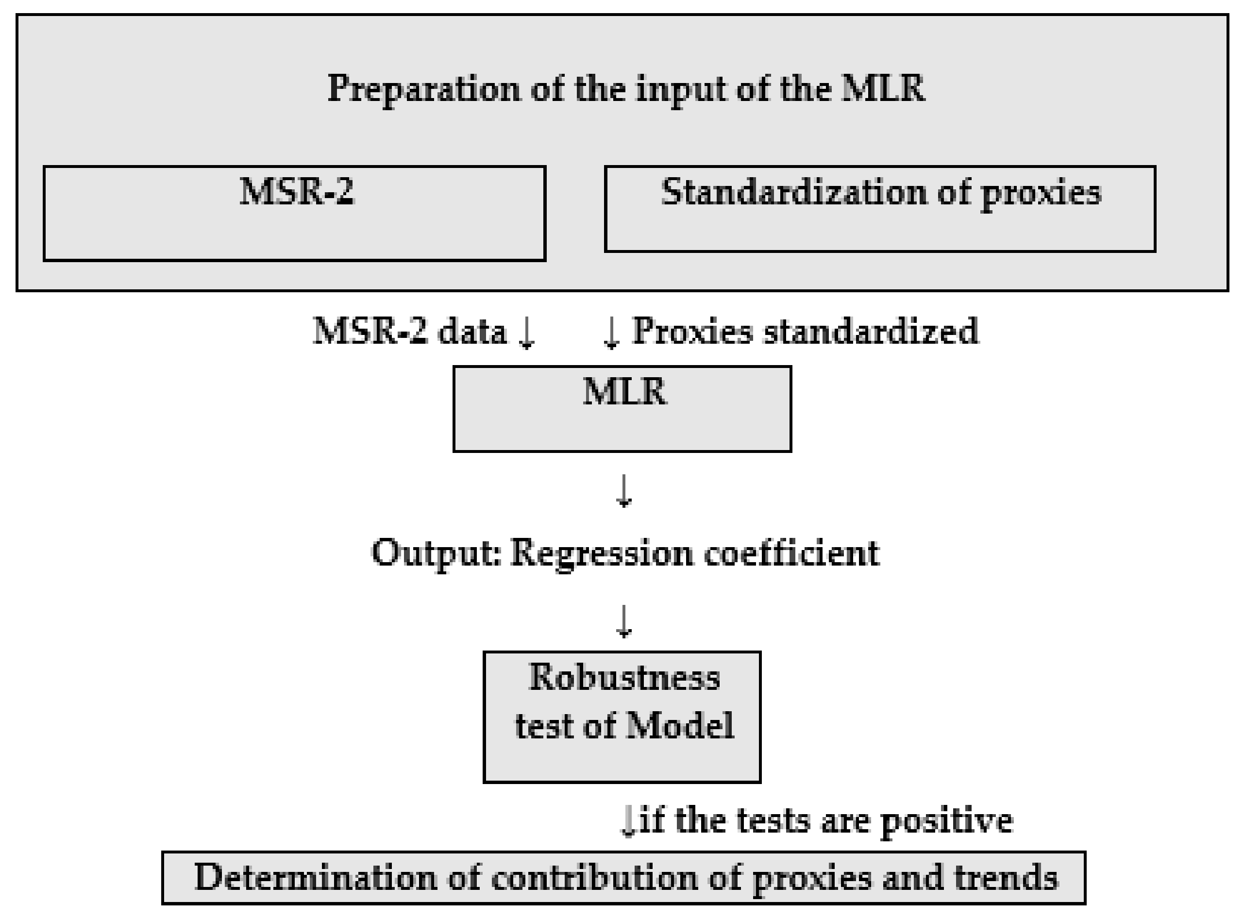
3. Methodology
- ■
- Y(t) is the monthly TOC average,
- ■
- t designates the month between 1 and 504, i.e., the number of months between 1979 and 2020,
- ■
- K denotes the constant (intercepts) of the model,
- ■
- Cproxy designates the regression coefficients of different proxies, and
- ■
- ∈ (t) is the total of the residuals of the ozone anomalies.
- ■
- The explained variable is the monthly average TOC for the time series and constitutes the input value of the MLR; and
- ■
- The explanatory variables are the Annual Oscillation (AnO), the Semi-Annual Oscillation (SAnO), the anomalies of the Solar Flux (SF), the El Niño–Southern Oscillation (ENSO), the Quasi-Biennial Oscillation at 30 mb (QBO30), the Quasi-Biennial Oscillation at 10 mb (QBO10), and the linear trend functions (T1; T2). The QBO, ENSO, and SF explanatory variables linked to the contribution of dynamical and radiative processes on total ozone interannual variability are the usual ones already used in different studies [22,34].
- ■
- t is the rank of the months in the time series, and
- ■
- I is the phasing coefficient between the TOC time signal and the AnO or SanO.
4. Results and Discussion
4.1. Evaluation of the MLR Model
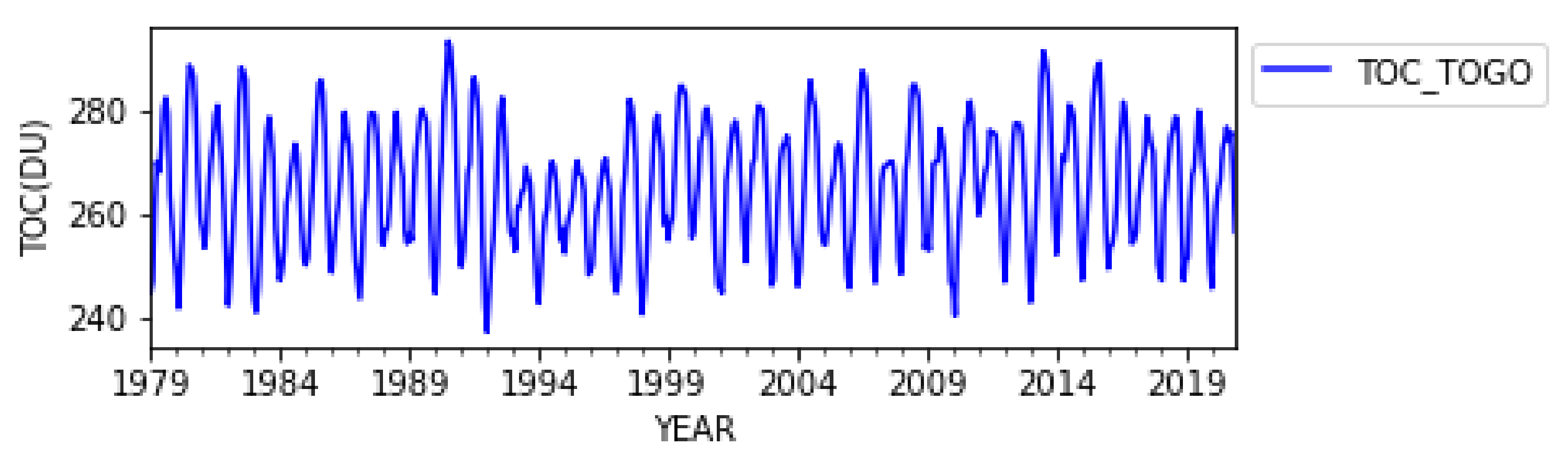
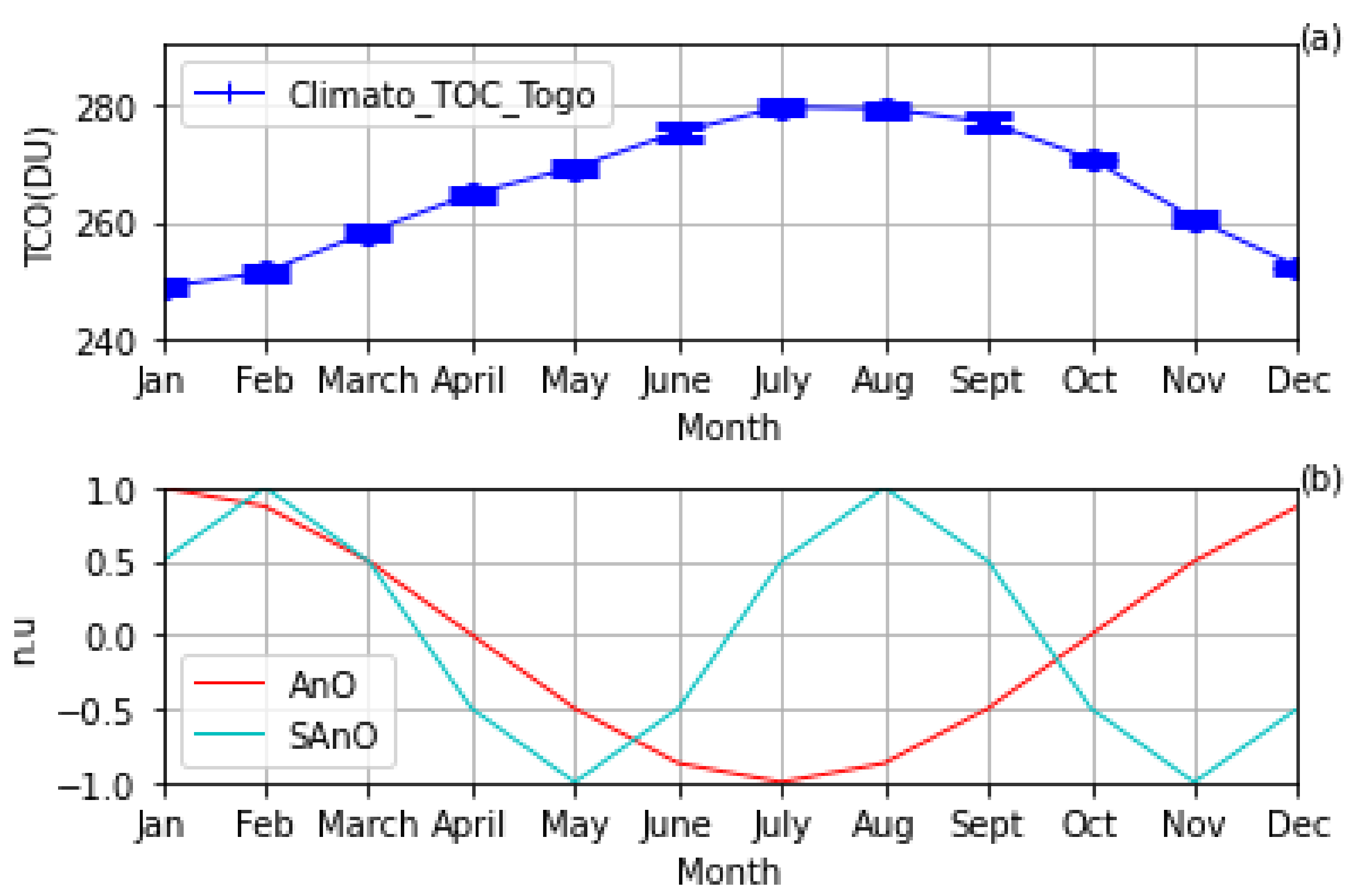
4.2. Ozone above Togo
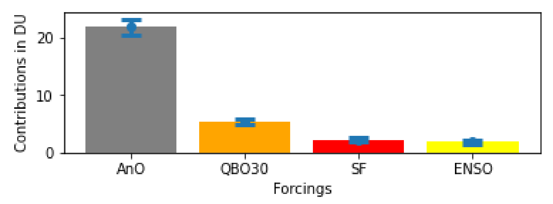
4.3. Contributions of Different Proxies
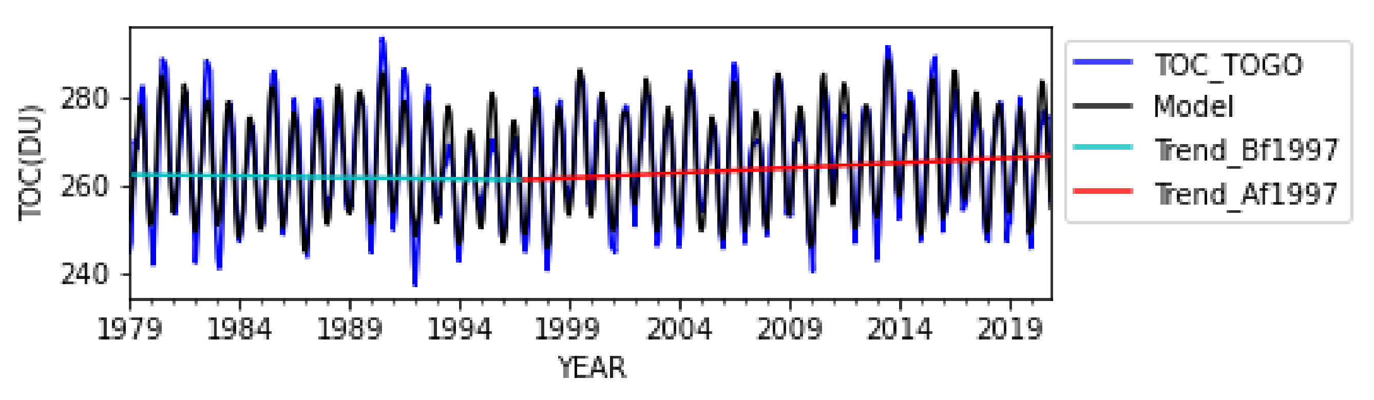
4.4. Interannual Trends
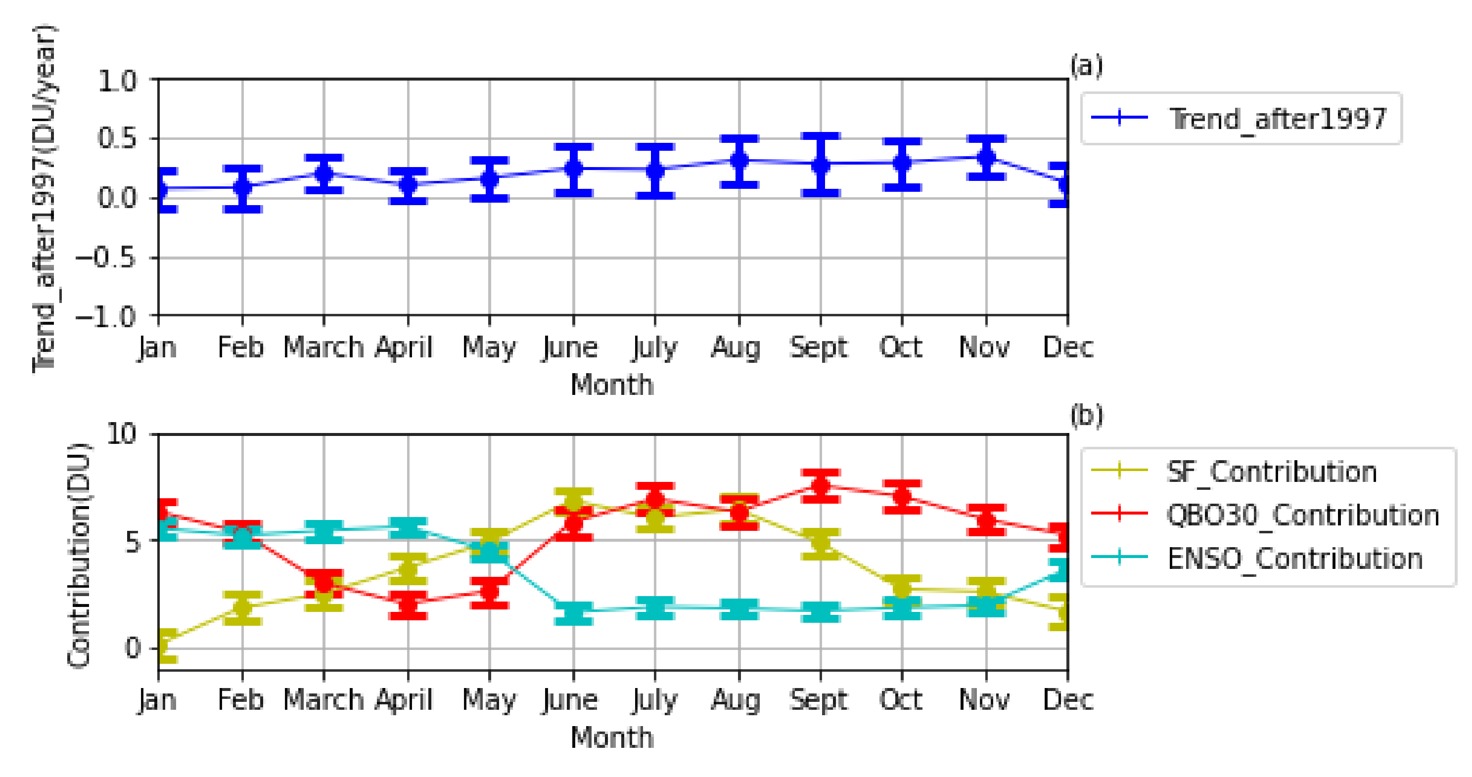
4.5. Trend by Month
5. Conclusions
Author Contributions
Funding
Institutional Review Board Statement
Data Availability Statement
Acknowledgments
Conflicts of Interest
Appendix A
References
- McMichael, A.J.; Haines, J.A.; Slooff, R.; Sari Kovats, R.; World Health Organization. Climate Change and Human Health: An Assessment; No. WHO/EHG/96.7; World Health Organization: Geneva, Switzerland, 1996. [Google Scholar]
- Kakani, V.G.; Reddy, K.R.; Zhao, D.; Sailaja, K. Field crop responses to ultraviolet-B radiation: A review. Agric. For. Meteorol. 2003, 120, 191–218. [Google Scholar] [CrossRef]
- Vernet, M.; Brody, E.A.; Holm-Hansen, O.; Mitchell, B.G. The response of Antarctic phytoplankton to ultraviolet radiation: Absorption, photosynthesis, and taxonomic composition. In Ultraviolet Radiation in Antarctica: Measurements and Biological Effects; Weiler, C.S., Penhale, P.A., Eds.; American Geophysical Union: Washington, DC, USA, 1994; pp. 143–158. [Google Scholar]
- Butchart, N. The Brewer-Dobson circulation. Rev. Geophys. 2014, 52, 157–184. [Google Scholar] [CrossRef]
- Harris, N.R.; Kyrö, E.; Staehelin, J.; Brunner, D.; Andersen, S.-B.; Godin-Beekmann, S.; Dhomse, S.; Hadjinicolaou, P.; Hansen, G.; Isaksen, I.; et al. Ozone trends at northern mid- and high latitudes—A European perspective. Geophys. Ann. 2008, 26, 1207–1220. [Google Scholar] [CrossRef] [Green Version]
- Weber, M.; Dikty, S.; Burrows, J.; Garny, H.; Dameris, M.; Kubin, A.; Abalichin, J.; Langematz, U. The Brewer-Dobson circulation and total ozone from seasonal to decacadal time scale. Atmos. Chem. Phys. 2011, 11, 11221–11235. [Google Scholar] [CrossRef] [Green Version]
- Montzka, S.; Reimannander, S.; Engel, A.; Kruger, K.; Simon, O.; Sturges, W.; Blake, D.; Dorf, M.; Fraser, P.; Froidevaux, L.; et al. Ozone-Depleting Substances (ODSs) and Related Chemicals, Chapter 1. In Scientific Assessment of Ozone Depletion: 2010, Global Ozone Research and Monitoring Project-Report No.52; World Meteorological Organization: Geneva, Switzerland, 2011. Available online: https://tsapps.nist.gov/publication/get_pdf.cfm?pub_id=909747 (accessed on 4 December 2022).
- Kuttippurath, J.; Lefèvre, F.; Pommereau, J.; Roscoe, H.K.; Goutail, F.; Pazmiño, A.; Shanklin, J.D. Antarctic ozone loss in 1979–2010: First sign of ozone recovery. Atmos. Chem. Phys. 2013, 13, 1625–1635. [Google Scholar] [CrossRef] [Green Version]
- Krzyścin, W.J.; Baranowski, D.B. Signs of the ozone recovery based on multi sensor reanalysis of total ozone for the period 1979–2017. Atmos. Environ. 2019, 199, 334–344. [Google Scholar] [CrossRef]
- Reinsel, G.C.; Miller, A.J.; Weatherhead, E.C.; Flynn, L.E.; Nagatani, R.M.; Tiao, G.C.; Wuebbles, D.J. Trend analysis of total ozone data for turnaround and dynamical contributions. J. Geophys. Res. 2005, 110, D16306. [Google Scholar] [CrossRef]
- Farman, J.; Gardiner, B.; Shanklin, J. Large losses of total ozone in Antarctica reveal seasonal ClOx/NOx interaction. Nature 1985, 315, 207–210. [Google Scholar] [CrossRef]
- World Meteorological Organization (WMO). Scientific Assessment of Ozone Depletion: 2014; World Meteorological Organization (WMO): Geneva, Switzerland, 2014. [Google Scholar]
- Solomon, S.; Garcia, R.; Rowland, F.; Donald, J. On the depletion of Antarctic ozone. Nature 1986, 321, 755–758. [Google Scholar] [CrossRef] [Green Version]
- McElroy, M.; Salawitch, R.; Wofsy, S.; Logan, J. Reductions of Antarctic ozone due to synergistic interactions of chlorine and bromine. Nature 1986, 321, 759–762. [Google Scholar] [CrossRef]
- UNEP. Handbook for the Montreal Protocol on Substances that Deplete the Ozone Layer, 13th ed.; Ozone Secretariat: Nairobi, Kenya, 2019. [Google Scholar]
- WMO (World Meteorological Organization). Scientific Assessment of Ozone Depletion: 2018, Global Ozone Research and Monitoring; Project-Report No.58; WMO (World Meteorological Organization): Geneva, Switzerland, 2018. [Google Scholar]
- Klobas, J.E.; Weisenstein, D.K.; Salawitch, R.J.; Wilmouth, D.M. Reformulating the bromine alpha factor and equivalent effective stratospheric chlorine (EESC): Evolution of ozone destruction rates of bromine and chlorine in future climate scenarios. Atmos. Chem. Phys. 2020, 20, 9459–9471. [Google Scholar] [CrossRef]
- Newman, A.; Daniel, J.S.; Waugh, D.W.; Nash, E.R. A new formulation of equivalent effective stratospheric chlorine (EESC). Atmos. Chem. Phys. 2007, 7, 3963–4000. [Google Scholar]
- Braesicke, P.; Neu, J.L.; Fioletov, V.E.; Godin-Beekmann, S.; Hubert, D.; Petropavlovskikh, I.; Shiotani, M.; Sinnhuber, B.M.; Ball, W.; Chang, K.L.; et al. Update on Global Ozone: Past, Present, and Future, Chapter 3. In WMO Scientific Assessment of Ozone Depletion (2018); WMO: Geneva, Switzerland, 2018; Volume 58. [Google Scholar]
- Ball, W.T.; Alsing, J.; Mortlock, D.J.; Staehelin, J.; Haigh, J.D.; Peter, T.; Tummon, F.; Stübi, R.; Stenke, A.; Anderson, J.; et al. Evidence for a continuous decline in lower stratospheric ozone offsetting ozone layer recovery. Atmos. Chem. Phys. 2018, 18, 1379–1394. [Google Scholar] [CrossRef] [Green Version]
- Smyshlyaev, S.; Galin, V.Y.; Blakitnaya, A.; Jakovlev, A.R. Numerical Modeling of the Natural and Manmade Factors Influencing Past and Current Changes in Polar, and Tropical Ozone. Atmosphere 2020, 11, 76. [Google Scholar] [CrossRef] [Green Version]
- Coldewey-Egbers, M.; Loyola, D.G.; Lerot, C.; Roozendael, M.V. Global, regional and seasonal analysis of total ozone trends derived from the 1995–2020 GTO-ECV climate data record. Atmos. Chem. Phys. 2022, 22, 6861–6878. [Google Scholar] [CrossRef]
- Meul, S.; Dameris, M.; Langematz, U.; Abalichin, J.; Kerschbaumer, A.; Kubin, A.; Oberländer-Hayn, S. Impact of rising greenhouse gas concentrations on future tropical ozone and UV exposure. Geophys. Res. Lett. 2016, 43, 2919–2927. [Google Scholar] [CrossRef] [Green Version]
- Szeļag, M.E.; Sofieva, V.F.; Degenstein, D.; Roth, C.; Davis, S.; Froidevaux, L. Seasonal stratospheric ozone trends over 2000–2018 derived from several merged data sets. Atmos. Chem. Phys. 2020, 20, 7035–7704. [Google Scholar]
- Weber, M.; Arosio, C.; Coldewey-Egbers, M.; Fioletov, V.E.; Frith, S.M.; Wild, J.D.; Tourpali, K.; Burrows, J.; Loyola, D. Global total ozone recovery trends attributed to ozone-depleting substance (ODS) changes derived from. Atmos. Chem. Phys. 2022, 22, 6843–6859. [Google Scholar] [CrossRef]
- Ramaswamy, V.; Schwarzkopf, M.D.; Randel, W.J.; Santer, B.D.; Soden, B.J.; Stenchikov, G.L. Anthropogenic and natural influences in the evolution of lower stratospheric cooling. Science 2006, 311, 1138–1141. [Google Scholar] [CrossRef]
- Bencherif, H.; Toihir, A.; Mbatha, N.; Sivakumar, V.; du Preez, D.; Bègue, N.; Coetzee, G. Ozone Variability and Trend Estimates from 20-Yearsof Ground-Based and Satellite Observations at Irene Station, South Africa. Atmosphere 2020, 11, 1216. [Google Scholar] [CrossRef]
- Pazmiño, A.; Godin-Beekmann, S.; Hauchecorne, A.; Claud, C.; Khaykin, S. Multiple symptoms of total ozone recovery inside the Antarctic. Atmos. Chem. Phys. 2018, 18, 7557–7572. [Google Scholar]
- Nair, J.; Godin-Beekmann, S.; Kuttippurath, J.; Ancellet, G.; Goutail, F.; Pazmiño, A.; Froidevaux, L.; Zawodny, J.M.; Evans, R.D.; Wang, H.J.; et al. Ozone trends derived from the total column and vertical profiles at a northern mid-latitude station. Atmos. Chem. Phys. 2013, 13, 7081–7112. [Google Scholar] [CrossRef] [Green Version]
- Van Der A, R.J.; Allaart, M.A.F.; Eskes, H.J. Multi sensor re-analysis of total ozone. Atmos. Chem. Phys. 2010, 10, 11277–11294. [Google Scholar] [CrossRef]
- Van Der A, R.J.; Allaart, M.A.F.; Eskes, H.J. Extended and refined multi sensor reanalysis of total ozone for the period 1970–2012. Atmos. Meas. Tech. 2015, 8, 3021–3035. [Google Scholar] [CrossRef] [Green Version]
- R Core Team (2022) R: A Language and Environment for Statistical Computing; R Foundation for Statistical Computing: Vienna, Austria. Available online: https://www.R-project.org/ (accessed on 16 August 2022).
- Tiao, G.; Reinse, G.; Xu, D.; Pedrick, J.; Zhu, X.; Miller, A.; Deluis, I.J.; Mateer, C.; Wuebbles, D. Effects of correlation and temporal sampling schemes on estimates of trend and spatial correlation. J. Geophys. Res. 1990, 95, 507–517. [Google Scholar] [CrossRef]
- Toihir, A.M.; Portafaix, T.; Sivakumar, V.; Bencherif, H.; Pazmino, A.; Bègue, N. Variability and trend in ozone over the southern tropics and subtropics. Ann. Geophys. 2018, 36, 381–404. [Google Scholar] [CrossRef] [Green Version]
- Olsen, M.A.; Manney, G.L.; Liu, J. The ENSO and QBO impact on ozone variability and stratosphere-Troposphere exchange relative to the subtropical jets. J. Geophys. Res. Atmos. 2019, 124, 7379–7392. [Google Scholar] [CrossRef]
- Han, Z.; Chongping, J.; Libo, Z. QBO Signal in total ozone over Tibet. Adv. Atmos. Sci. 2000, 17, 562–568. [Google Scholar] [CrossRef]
- Chehade, W.; Weber, M.; Burrows, J.P. Total ozone trends and variability during 1979–2012 from merged data sets of various satellites. Atmos. Chem. Phys. 2014, 14, 7059–7074. [Google Scholar] [CrossRef] [Green Version]
- Jin, D.; Kirtman, B. The impact of ENSO periodicity on North Pacific SST variability. Clim. Dyn. 2010, 34, 1015–1039. [Google Scholar] [CrossRef]
- Dijkstra, H.A. The ENSO phenomenon: Theory and mechanisms. Adv. Goesci. 2006, 6, 3–15. [Google Scholar] [CrossRef] [Green Version]
- Shiotani, M. Annual, quasi-biennial, and El Nino-Southern Oscillation (ENSO) time-scale variations in equatorial total ozone. J. Geophys. Res. 1992, 97, 7625–7633. [Google Scholar] [CrossRef]
- Randel, W.J.; Garcia, R.R.; Calvo, N.; Marsh, D. ENSO influence on zonal mean temperature and ozone in the tropicallower stratosphere. Geophys. Res. Lett. 2009, 36, L15822. [Google Scholar] [CrossRef]
- Bourassa, A.E.; Degenstein, D.A.; Randel, W.J.; Zawodny, J.M.; Kyrölä, E.; McLinden, C.A.; Sioris, C.E.; Roth, C.Z. Trends in stratospheric ozone derived from merged SAGE II and Odin-OSIRIS satellite observations. Atmos. Chem. Phys. 2014, 14, 6983–6994. [Google Scholar] [CrossRef] [Green Version]
- Li, K.-F.; Jiang, X.; Liang, M.-C.; Yun, Y.L. Simulation of solar-cycle response in tropical total column ozone using. Atmos. Chem. Phys. 2012, 12, 1867–1893. [Google Scholar]
- Bojkov, R.D.; Fioletov, V.E. Total ozone variations in the tropical belt: An application for quality of ground based measurements. Mefeorology Atmos. Phys. 1996, 58, 223–240. [Google Scholar] [CrossRef]
- Labitzke, K. The global signal of the 11-year solar cycle in the stratosphere: Observations and models: Differences between solar maxima and minima. Meteorol. Z. 2001, 10, 83–90. [Google Scholar] [CrossRef]
- Gray, L.J.; Beer, J.; Geller, M.; Haigh, J.D.; Lockwood, M.; Matthes, K.; Cubasch, U. Solar influences on climate. Rev. Geophys. 2010, 48, 2010. [Google Scholar] [CrossRef] [Green Version]
- Soukharev, B.E.; Hood, L.L. Solar cycle variation of stratospheric ozone: Multiple regression analysis of long-term satellite data sets and comparisons with models. J. Geophys. Res. 2006, 111, D20314. [Google Scholar] [CrossRef] [Green Version]
- Reinsel, G.C.; Weatherhead, E.; Tiao, G.C.; Miller, A.J.; Nagatani, R.M.; Wuebbles, D.J.; Flynn, L.E. On detection of turnaround and recovery in trend of ozone. J. Geophys. 2002, 107, 4078. [Google Scholar] [CrossRef]
- Petropavlovskikh, I.; Godin-Beekmann, S.; Hubert, D.; Damadeo, R.; Hassler, B.; Sofieva, V. SPARC/IO3C/GAW Report on Long-term Ozone Trends and Uncertainties in the Stratosphere. PARC/IO3C/GAW, 2019: SPARC Report No. 9, GAW Report No. 241, WCRP-17/2018. Available online: www.sparc-climate.org/publications/sparc-reports (accessed on 11 November 2022).
- Steinbrecht, W.; Hassler, B.; Claude, H.; Winkler, P.; Stolarski, R.S. Global distribution of total ozone and lower stratospheric temperature variations. Atmos. Chem. Phys. 2003, 3, 1421–1438. [Google Scholar] [CrossRef] [Green Version]
- Zerefos, C.S.; Bais, A.F.; Ziomas, I.C.; Bojkov, R.D. On the relative importance of Quasi-Biennial Oscillation and El Ni ño/Southern Oscillation in the Revised Dobson Total Ozone Records. J. Geophys. Res. 1992, 97, 10135–10144. [Google Scholar] [CrossRef]
- Poulain, V.; Bekki, S.; Marchand, M.; Chipperfield, M.; Khodri, M.; Lefèvre, F.; Dhomse, S. Evaluation of the Inter-Annual Variability of Stratospheric Chemical Composition in Chemistry-Climate Models Using Ground-Based Multi Species Time. J. Atmos. Sol. Terr. Phys. 2016, 145, 61–84. [Google Scholar] [CrossRef] [Green Version]
- Ball, W.T. (QOS) Evidence that tropical total column ozone no longer represents stratospheric changes. Personal communication, 2021. [Google Scholar]
- Godin-Beekmann, S.; Azouz, N.; Sofieva, V.; Hubert, D.; Petropavlovskikh, I.; Effertz, P.; Ancellet, G.; Degenstein, D.A.; Zawada, D.; Froidevaux, L.; et al. Updated trends of thozone vertical distribution in the in the 60° S–60° N latitude range based an LOTUS regression model. Atmos. Chem. Phys. 2022, 22, 11657–11673. [Google Scholar] [CrossRef]
- Thompson, A.M.; Stauffer, R.M.; Wargan, K.; Witte, J.C.; Kollonige, D.E.; Ziemke, J.R. Regional and Seasonal Trends in Tropical Ozone From SHADOZ Profiles: Reference for Models and Satellite Products. J. Geophys. Res. Atmos. 2021, 126, e2021JD034691. [Google Scholar] [CrossRef]
- Leventidou, E.; Weber, M.; Eichmann, K.-U.; Burrows, J.; Heue, K.; Thompson, A.M. Harmonisation and trends of 20-year tropical tropospheric ozone data. Atmos. Chem. Phys. 2018, 18, 9189–9205. [Google Scholar] [CrossRef] [Green Version]
- Gaudel, A.; Cooper, O.R.; Ancellet, G.; Barret, B.; Boynard, A.; Burrows, J.; Clerbaux, C.; Coheur, P.-F.; Cuesta, J.; Cuevas, E.; et al. Tropospheric Ozone Assessment Report: Present-day distribution and trends of tropospheric ozone relevant to climate and global atmospheric chemistry model evaluation. Elem. Sci. Anthr. 2018, 6, 39. [Google Scholar] [CrossRef] [Green Version]
- Tarasick, D.; Galbally, I.E.; Cooper, O.R.; Schultz, M.G.; Ancellet, G.; Leblanc, T.; Wallington, T.J.; Ziemke, J.; Liu, X.; Steinbacher, M.; et al. Tropospheric Ozone Assessment Report: Tropospheric ozone from 1877 to 2016, observed levels, trends and uncertainties. Elem. Sci. Anthr. 2019, 7, 39. [Google Scholar] [CrossRef] [Green Version]
- Butchart, N.; Scaife, A.; Bourqui, M.; Grandpré, J.d.; Hare, S.; Kettleborough, J.; Langematz, U.; Manzini, E.; Sassi, F.; Shibata, K.; et al. Simulations of anthropogenic change in the strength of the Brewer-Dobson circulation. Clim. Dyn. 2006, 27, 727–741. [Google Scholar] [CrossRef]
- Eyring, V.; Shepherd, T.; Waugh, D. (Eds.) SPARC, 2010: SPARC CCMVal Report on the Evaluation of Chemistry-Climate Models. SPARC Report No. 5, WCRP-30/2010, WMO/TD—No. 40. Available online: www.sparc-climate.org/publications/sparc-reports/ (accessed on 4 December 2022).
- Montzka, S.; Dutton, G.; Yu, P.; Ray, E.; Portmann, R.W.; Daniel, J.S.; Kuijpers, L.; Hall, B.D.; Mondeel, D.; Siso, C.; et al. An unexpected and persistent increase in global emissions of ozone-depleting CFC-11. Nature 2018, 557, 413–417. [Google Scholar] [CrossRef] [Green Version]
- Okoro, E.; Okeke, F.; Omeje, L. Investigating Contributions of Total Column Ozone Variation on Some Meteorological Parameters in Nigeria. Atmos. Clim. Sci. 2022, 12, 132–149. [Google Scholar] [CrossRef]
- Verma, S.; Yadava, P.K.; Lal, D.M.; Mall, R.K.; Kumar, H.; Payra, S. Role of Lightning NOx in Ozone Formation: A Review. Pure Appl. Geophys. 2021, 178, 1425–1443. [Google Scholar] [CrossRef]


| Proxy | Source | Characteristics |
|---|---|---|
| QBO 30 and 10 | Freie Universität Berlin Department of Earth Sciences/Institute of Meteorology/Atmospheric Dynamics https://www.geo.fu-berlin.de/met/ag/strat/produkte/qbo/qbo.dat accessed on 22 September 2021 | Monthly mean quasi-biennial oscillation at 30 mb and 10 mb |
| ENSO_MEI | NOAA Physical Science Laboratory https://psl.noaa.gov/enso/mei/data/meiv2.data accessed on 17 September 2021 | Monthly average of the Multivariate ENSO Index Version 2 |
| SF | The National Research Council of Canada Dominion Radio Astrophysical Observatory in Penticton ftp://ftp.geolab.nrcan.gc.ca/data/solar_flux/monthly_averages/solflux_monthly_average.txt ftp://ftp.seismo.nrcan.gc.ca/spaceweather/solar_flux/monthly_averages/solflux_monthly_average.txt both accessed on 25 November 2021 | Monthly averages of Solar Flux at a 10.7 cm wavelength |
| R2 | R2 Adjusted | p-Value |
|---|---|---|
| 76% | 75% | <5.37 × Exp(−147) |
| Proxies | AnO | SAnO | QBO 30 | QBO10 | SF | ENSO |
|---|---|---|---|---|---|---|
| Regression coefficients in the DU | −15.38 ± 0.71 | 0.59 ± 0.71 | 9.39 ± 0.29 | 0.98 ± 0.31 | 6.62 ± 0.17 | −5.22 ± 0.18 |
| Contributions to the DU | 21.84 ± 1.42 *** | 0.84 ± 1.42 | 5.35 ± 0.57 *** | 0.60 ± 0.61 | 2.25 ± 0.34 *** | 1.88 ± 0.36 *** |
| Contribution in % | 67 | 3 | 16 | 2 | 7 | 6 |
| QBO30 mb | ENSO | SF | Trend | Adjusted R2 | ρ | |
|---|---|---|---|---|---|---|
| January | 6.31 ± 0.46 | −5.54 ± 0.36 | −0.12 ± 0.60 | 0.07 ± 0.16 | 55% | 0.20 |
| February | 5.36 ± 0.46 | −5.21 ± 0.36 | 1.84 ± 0.64 | 0.08 ± 0.18 | 55% | 0.00 |
| March | 2.99 ± 0.48 | −5.44± 0.36 | 2.50 ± 0.59 | 0.20 ± 0.14 | 64% | 0.10 |
| April | 2.02 ± 0.53 | −5.63 ± 0.36 | 3.70 ± 0.56 | 0.10 ± 0.13 | 68% | 0.20 |
| May | 2.62± 0.58 | −4.49 ± 0.36 | 4.89 ± 0.53 | 0.16 ± 0.16 | 56% | 0.10 |
| June | 5.82 ± 0.62 | −1.62 ± 0.37 | 6.83 ± 0.55 | 0.24 ± 0.20 | 48% | 0.00 |
| July | 6.92 ± 0.64 | 1.89 ± 0.37 | 6.04 ± 0.50 | 0.23 ± 0.20 | 54% | 0.40 |
| August | 6.31 ± 0.65 | 1.82 ± 0.37 | 6.43 ± 0.58 | 0.31 ± 0.20 | 56% | 0.00 |
| September | 7.55± 0.63 | 1.69± 0.37 | 4.89 ± 0.59 | 0.28 ± 0.24 | 55% | 0.20 |
| October | 7.03 ± 0.62 | −1.85 ± 0.37 | 2.71± 0.60 | 0.29 ± 0.20 | 53% | 0.30 |
| November | 5.97± 0.57 | −1.95 ± 0.37 | 2.59 ± 0.62 | 0.34 ± 0.16 | 53% | 0.00 |
| December | 5.23 ± 0.51 | −3.63 ± 0.37 | 1.68 ± 0.65 | 0.12 ± 0.16 | 37% | 0.10 |
Publisher’s Note: MDPI stays neutral with regard to jurisdictional claims in published maps and institutional affiliations. |
© 2022 by the authors. Licensee MDPI, Basel, Switzerland. This article is an open access article distributed under the terms and conditions of the Creative Commons Attribution (CC BY) license (https://creativecommons.org/licenses/by/4.0/).
Share and Cite
Ayassou, K.; Pazmiño, A.; Sabi, K.; Bazureau, A.; Godin-Beekmann, S. Evolution of Ozone above Togo during the 1979–2020 Period. Atmosphere 2022, 13, 2066. https://doi.org/10.3390/atmos13122066
Ayassou K, Pazmiño A, Sabi K, Bazureau A, Godin-Beekmann S. Evolution of Ozone above Togo during the 1979–2020 Period. Atmosphere. 2022; 13(12):2066. https://doi.org/10.3390/atmos13122066
Chicago/Turabian StyleAyassou, Koffi, Andrea Pazmiño, Kokou Sabi, Ariane Bazureau, and Sophie Godin-Beekmann. 2022. "Evolution of Ozone above Togo during the 1979–2020 Period" Atmosphere 13, no. 12: 2066. https://doi.org/10.3390/atmos13122066
APA StyleAyassou, K., Pazmiño, A., Sabi, K., Bazureau, A., & Godin-Beekmann, S. (2022). Evolution of Ozone above Togo during the 1979–2020 Period. Atmosphere, 13(12), 2066. https://doi.org/10.3390/atmos13122066