Article

Active Air Monitoring for Understanding the Ventilation and Infection Risks of SARS-CoV-2 Transmission in Public Indoor Spaces

1
Global Centre for Clean Air Research (GCARE), School of Sustainability, Civil and Environmental Engineering, Faculty of Engineering and Physical Sciences, University of Surrey, Guildford GU2 7XH, UK
2
Institute for Sustainability, University of Surrey, Guildford GU2 7XH, UK
3
Centre for Mathematical Sciences, Department of Applied Mathematics and Theoretical Physics, University of Cambridge, Wilberforce Road, Cambridge CB3 0WA, UK
4
National Heart & Lung Institute, Imperial College London, London SW3 6LY, UK
5
Department of Materials Science and Engineering, Imperial College London, London SW7 2AZ, UK
6
Department of Life Sciences, Imperial College London, Silwood Park Campus, Buckhurst Road, Ascot SL5 7PY, UK
7
School of Medicine, University of Liverpool, Liverpool L69 3GE, UK
8
Earth Science and Engineering, Imperial College London, London SW7 2AZ, UK
*
Author to whom correspondence should be addressed.
Atmosphere 2022, 13(12), 2067; https://doi.org/10.3390/atmos13122067
Submission received: 6 November 2022 / Revised: 3 December 2022 / Accepted: 5 December 2022 / Published: 8 December 2022
(This article belongs to the Section Air Quality and Human Health)

Abstract

:
Indoor, airborne, transmission of SARS-CoV-2 is a key infection route. We monitored fourteen different indoor spaces in order to assess the risk of SARS-CoV-2 transmission. PM2.5 and CO2 concentrations were simultaneously monitored in order to understand aerosol exposure and ventilation conditions. Average PM2.5 concentrations were highest in the underground station (261 ± 62.8 μgm−3), followed by outpatient and emergency rooms in hospitals located near major arterial roads (38.6 ± 20.4 μgm−3), the respiratory wards, medical day units and intensive care units recorded concentrations in the range of 5.9 to 1.1 μgm−3. Mean CO2 levels across all sites did not exceed 1000 ppm, the respiratory ward (788 ± 61 ppm) and the pub (bar) (744 ± 136 ppm) due to high occupancy. The estimated air change rates implied that there is sufficient ventilation in these spaces to manage increased levels of occupancy. The infection probability in the medical day unit of hospital 3, was 1.6-times and 2.2-times higher than the emergency and outpatient waiting rooms in hospitals 4 and 5, respectively. The temperature and relative humidity recorded at most sites was below 27 °C, and 40% and, in sites with high footfall and limited air exchange, such as the hospital medical day unit, indicate a high risk of airborne SARS-CoV-2 transmission.

1. Introduction

Severe acute respiratory syndrome coronavirus 2 (SARS-CoV-2) is a single-stranded RNA virus that causes coronavirus disease 2019 (COVID-19) [1,2]. Table 1 presents various studies which have monitored PM2.5 and CO2 levels to estimate the risk of COVID infection transmission.
The first outbreak of COVID-19 was reported in December 2019, in Wuhan, China [13] and was declared as a pandemic on 11 March 2020 by the WHO. The lack of understanding of the disease, its transmission, progression, and the relative unavailability of drugs and vaccines forced governments across the world to impose travel and social restrictions, and lockdowns at various stages of the pandemic, to reduce the pressure on healthcare infrastructure and prevent deaths. Self-isolation, track and trace were some of the effective tools that were used to break the chain of transmission [14,15]. Some developed countries including the United States of America (USA), United Kingdom (UK) and Italy experienced the greatest initial impact of these tools [16]. It has been established that the virus can be transmitted during the incubation as well as infection [17,18]. Initially, close-range droplets and fomites were believed to be the key route of transmission and, consequently, governments across the world-imposed lockdowns with the recommendation of 2-m interpersonal distancing, social distancing, and good hygiene practices [19]. It is now widely accepted that airborne transmission is also a key route for the spread of infection [20,21,22]. Experimental studies carried out using air samplers placed close to COVID patients have detected SARS-CoV-2 RNA on airborne particles [23,24]. The risk of infection is higher in indoor spaces where the majority of transmission occurs [25] and improved building ventilation could be an effective tool to reduce this risk [26]. In some hospitals, for example, where ventilation is poor, portable air cleaners carrying high-efficiency particulate air (HEPA) filters can be considered to provide optimal ventilation [27].
Ventilation plays a critical role in reducing indoor airborne disease transmission. Infection risk estimation in a mixed ventilation environment requires real time ventilation rates which are difficult to obtain in non-laboratory, real-world scenarios. We all produce and exhale CO2 which can be used as a marker for estimating the ventilation rate, and therefore the risk of SARS-CoV-2 transmission [28]. Though, indoor CO2 is a good marker for ventilation [29], airborne PM2.5 has strong links with the spread of COVID-19, including hospitals [30]. Therefore, we measured the concentrations of both PM2.5 and CO2. The aim of this paper is to assess environmental CO2 levels in indoor hot spots such as busy, essential, working public spaces, to understand the ventilation types, rate, dispersion mechanism, and to identify the risk of transmission of airborne diseases such as COVID-19. To achieve this, we monitored PM2.5 and CO2 in all sites and, in a limited number of sites, in tandem, we recorded the number of occupants/CO2 sources. We combined the sources and time-series of CO2 to estimate the ventilation efficiency of these spaces, and finally, the risk of transmission.

2. Materials and Methods

2.1. Description of the Sampling Area

The study was carried out in the Greater London area. The selected sampling sites were working indoor spaces including hospitals (2 ICUs, 1 respiratory ward, 2 emergency rooms and 1 outpatient ward), schools/research institutes (20%), pubs/bars (10%), and indoors of bus/train stations (10%). The concentration levels of PM2.5 and CO2 were collected at these sampling sites. We refer to the sites by their code names, as classified and listed in Table 2, to maintain their anonymity. Table 2 and Table S2 also presents a brief description of each sampling site, date of sampling, and the sampling duration. The sampling days’ corresponding number of recorded cases and infection prevalence (%) were calculated against the London population and the cumulative days since 11 February 2020 (Table S1). We collected data for 3–10 h during working hours (e.g., 08:00 h to 17:00 h) on sites where instruments needed to be supervised. On unsupervised sites, we collected data for 24 h.
Hospital #1 (respiratory ward)—(HS1-RW): Located alongside a major arterial road. Samples taken in a six-bed respiratory ward located on the 5th floor of the building. During the monitoring period, four out of six beds were occupied by COVID-19 patients who were not receiving supplemental oxygen support. The ward was mechanically ventilated, and data was collected for a period of 2 h 30 min.
Hospital #1 (intensive care unit (ICU))—(HS1-ICU): Located on the 11th floor. Two beds occupied by COVID-19 patients on ventilators, attended periodically by medical staff. The ICU had negative pressure ventilation and a room volume of 71 m3. The sampling was carried out in three different runs, each with different sampling duration as listed in Table 2.
Hospital #1 (accident and emergency room)—(HS1-AER): Located in an accident and emergency room on the ground floor. Room was ventilated mechanically with a room volume of ≅126 m3 and a seating capacity of 29, with an occupancy rate ranging from 5 to 14 personnel (including one nurse organising the patients for their appointments). The air pollutants data were collected for a duration of around 7 h.
Hospital #2 (ICU): An 18-bed adult intensive care unit (AICU) located on the third floor, equipped with negative pressure ventilation and room volume of 65 m3. The sampling was carried out for 5 h and 35 min to collect the air pollutants data.
Hospital #3 (medical day unit)—(HS3-MDU): Waiting room for cancer patients awaiting treatment, located on the ground floor. The room was mechanically ventilated with a volume of ~604 m3 and containing 50 chairs (for patients waiting) and 24 recliners (for patients receiving treatment) with an average of around 12 to 14 patients waiting from 08:30 h to 12:30 h. PM2.5 and CO2 levels were monitored in three different runs for three different durations as listed in Table 2.
Hospital #4 (emergency/outpatient room)—(HS4-EOM): Emergency and outpatient waiting room on the ground floor, located close to a busy road. The room was mechanically ventilated, with a volume of ≅350 m3. Occupancy was around 12 to 30 personnel (including three staffs in the reception area and one nurse), with a higher footfall from 13:00 to 17:00 h. The average patient waiting time was around 7 to 10 min. Two sampling runs were carried out to measure the concentrations of PM2.5 and CO2 for different durations as detailed in Table 2.
Hospital #5 (outpatient waiting room)—(HS5-OPR): Outpatient waiting room on the ground floor close to a minor road connecting to a busy road. The waiting room had a seating capacity of 19 and was busy between 09:30 h and 12:30 h with an average of 15 patients/carers and 6 medical personnel. The room was mechanically ventilated with a volume of ≅641 m3. The data collection involves four different sampling runs to collect the air pollutants data, which is listed in Table 2.
Research Institute—(RI): Microscopy suite of a research institute situated in West London on the ground floor. Samplers were placed in the corridor of the suite, which has 7 microscope rooms with at least one person per room. The whole suite was mechanically ventilated with a volume of ≅311 m3. The footfall was in the range of 3 to 4 people at a time. The sampling was carried out during the weekend for a total duration of around 73 h.
School—(SCH): A South-London junior school for children aged between 7 to 11, located approximately 400 m away from the busy road. The sampling area was mechanically ventilated, and the samplers were placed in the classroom corridor on the ground floor. Data acquisition was carried out continuously for a period of 30 h, including school hours.
Pub/Restaurant—(PR): Seating capacity of 120 with a volume of ~1613 m3 on the ground floor. The building housing the pub, situated in west-central London, was mechanically ventilated, with additional ventilation from an external door opening (1.1 m wide). We monitored the space during the England vs. Denmark European Cup semi-final match. We started data acquisition an hour prior to the match; although footfall varied (between 20–100 people) during the monitoring period, the number of occupants were counted and recorded every hour. The monitoring was carried out for a duration of around 4 h.
Train station (main concourse)—(TSM): A major Central London railway terminus at ground level with access to the Underground Train network. Samplers were placed near the information boards, where footfall and stationary time of passengers is higher than other areas of the station. The station is partially enclosed with natural ventilation. Concentrations of air pollutants were carried out in three different sampling runs with different durations listed in Table 2.
Underground station site #1—(UG-S1): Same site as TSM and serves as a connection from the underground network to the Great Western railway service. The sampling site was at the Gate Line Assistance Point (GLAP) located close to the passenger escalators leading to two underground platforms. The samplers were placed on the curb near the passenger flow and the footfall was very high, ranging from 800 to 1400 passengers during peak hours. The sampling was carried out in two sampling runs of 8 and 10 h.
Underground station site #2—(UG-S2): Near the ticket vending machine close to the entry gate to the underground station. The residence time of passengers is around 30 to 60 s for ticket payment in a high footfall area. The samplers were placed at around 1 m from the ticket machines and at a height of 1.5 m from the ground. Data was collected for around 10 h.
Underground station site #3—(UG-S3): Platform, 16 m below ground level. High footfall during peak hours and moderate footfall during non-peak hours. Passenger residence time of 1 to 3 min (waiting for train arrival). The samplers were placed at around 1.5 to 2 m from the train track (on the platform) and measurements were carried out for 10 h.

2.2. Measurement Instrumentation

PM2.5 and CO2 concentrations were measured by pDR-1500 and HOBO set up adjacent to each other on a tripod. The pDR-1500 (Thermo Scientific, Franklin, MA, United States of America (USA) measures size-segregated PM concentrations (e.g., PM10, PM4, PM2.5, PM1, etc.) using two different types of particle size-selective inlet cyclones. The instrument uses a highly sensitive nephelometric (i.e., photometric) monitoring technique to measure the respirable fraction of airborne dust in both indoor and outdoor environments. The instrument covers a wide measurement range of 0.001 mg.m−3 to 400 mg.m−3 with a precision of ±0.2% or ±0.0005 mg.m−3, whichever is larger, for 60 s averaging time and a flow rate of 1 to 3.5 L min−1. The pDR-1500 can log data from 1 s to 1 h intervals with up to 500,000 data points. The particle size measured depends on the flow rate at which the instrument is operated. In this study, we measured PM2.5 concentration at an interval of 60 s operating at a flow rate of 1.52 L.min−1. Additionally, we employed temperature and relative humidity (RH) sensors to mitigate the positive bias arising due to the elevated ambient RH [31]. The air sample was subsequently passed through a 37 mm glass microfiber filter (WhatmanTM 934-AHTM CAT No. 1827-037, with 2.0 μm pore size), from which PM were collected for gravimetric and chemical analyses. The filters containing the collected particles were desiccated for 24 h to remove any moisture, and then weighed using a microbalance (Mettler Toledo, XPR10), to determine the PM mass.
The CO2 concentrations were measured by using HOBO MX data logger and Temptop M2000C CO2 logger which uses a non-dispersive infrared (NDIR) self-calibrating CO2 sensor technology to measure the CO2 concentrations in the range of 0 to 5000 ppm with an accuracy of ±50 ppm or ±5% of reading. The instrument is equipped with a data logger at a logging rate of 1 s to 18 h. In this study, we logged data every 60 s. Additionally, integrated sensors provided temperature and RH data at the sampling sites. The CO2 concentrations and RH measurements were extracted from the HOBO MX logger, excluding the following sites: HS1-RW; HS1-ICU and HS2-ICU, where the temptop CO2 logger was used and the RH values were extracted from pDR1500.

2.3. Data Collection and Analysis

PM2.5, CO2 concentrations, temperature and RH data were collected from the sampling sites for a duration of 8 to 10 h (except in the pub, where the sampling was carried out for 4 h) in supervised sampling sites and for 24 h and more at unsupervised sampling sites, with sampling duration solely dependent on access to the sites. The PM2.5 data was extracted from pDR-1500 using the communication software application pDR port version 2.0.2.5 and processed using Microsoft Excel. The CO2 data was obtained using the software application ONSET HOBO mobileR for Android, version 2.0 build:1029. The collected CO2 data was the readout from the mobile application, extracted as a .csv file and then processed using Microsoft Excel Version 2205, Microsoft Corporation (Redmond, WA, USA) and ORIGIN 2020 (64 bit) version 9.7.0.185.

2.4. Estimation of Ventilation

CO2 is inherently produced by the occupants and other anthropogenic activities, which is constantly removed by building ventilation. To estimate the ventilation rate, we applied a CO2 component balance [32] with the following assumptions: (1) the indoor space is well mixed; (2) unless specifically mentioned, occupants are the only source of CO2; and (3) breathing rate, and the CO2 concentration in the exhaled breath is constant for each of the occupants.
C o Q ( t ) C ( t ) Q ( t ) + n ( t ) C b q = V d C ( t ) d t  
where C0 (ppm), C(t) (ppm), and Cb (ppm) are outdoor, indoor, and exhaled breath CO2 concentrations, respectively, q (m3 h−1) represents the breathing rate of occupants, n(t) is the number of occupants, V (m3) is the volume of the space and Q (m3 h−1) is the ventilation rate. Rearranging Equation (1) yields,
Q ( t ) =   n ( t ) C b q V d C ( t ) d t   ( C ( t ) C o )
The CO2 time series data allow us to calculate d C ( t ) d t , which enables us to estimate the ventilation rate (m3 h−1). In a fully mixed indoor environment, the component balance on CO2 produced by the occupants allows us to calculate the instantaneous ventilation rate, given by Equation (2). To calculate the ventilation rate, the raw data is filtered and smoothed using a Gaussian filter in Matlab (Figure 1). Subsequently, the smoothed data is differentiated to obtain realistic values of d C d t , and from Equation (2) the instantaneous ventilation rates. Air change per hour (ACH) can be calculated by A C H = Q V .

2.5. Evaluation of the Infection Risk

The potential risk of airborne disease transmission including SARS-CoV-2 is often estimated employing a fully mixed standard atmospheric box model/Wells-Riley model [33]. We assume that, initially, no virus was present in the space, the viral load builds over the period, and for the entire duration of risk estimation, the infected and susceptible individuals always occupy the space, and for this scenario, the probability of infection can be estimated using Equation (3). The viral load used here is expressed in terms of quanta emission rates (ERq, quanta h−1), which provides key information to simulate the dispersion of diseases in indoor environments [34].
R = ( 1 e I R × C a v g   × t × ( 1 f ) )
where R is probability of infection (%), IR is the breathing rate (0.8 m3 h−1) [35]), t is time of exposure (h); f is facemask efficiency (unless it is specified, we have used 50% as default) and Cavg is time-averaged quanta concentration (quanta m−3). Cavg is estimated based on site specific parameters such as quanta loss rate (λ = λk + λv + λd; h−1) due to virus inactivation (λk = 0.32 h−1), ventilation (λv; h−1) and surface deposition (λd = 0.3 h−1), virus emission rates per person (E: 2, 9.4, and 60.5 quanta h−1) and (V) volume of indoor space (m3), and is given by Equation (4),
C a v g = E × ( 1 f ) λ × v × ( 1 1 λ × t × ( 1 e ( λ × t ) ) )
The dimensions of the indoor space—the height (H); width (W) and length (L) in metres—was measured using a handheld laser enabled distance measurement device to calculate the room volume. The average ventilation rate in ACH (λv) is estimated (Section 3.2) for all sites using CO2 concentrations and occupancy data [36]. In the Wells-Riley model-based infection modelling, the input parameter, virus quanta generation rate pertains to uncertainties. The rate of exhaled virus quanta was assumed to be constant for an infectious person in a well-mixed environment for each activity (breathing, speaking and loud speaking). The quanta level in the background/fresh air was assumed to be zero during the infection probability estimation using Equation (3). We considered two extreme emission scenarios (i) resting—normal speaking; (ii) upper range of resting—loudly speaking to compare the probability of infection at different sampling sites with varied air change rates. In this study, we are considering the aerosol transmission risk and not the close-range droplet transmission for both the expiratory activities [37,38].

3. Results and Discussion

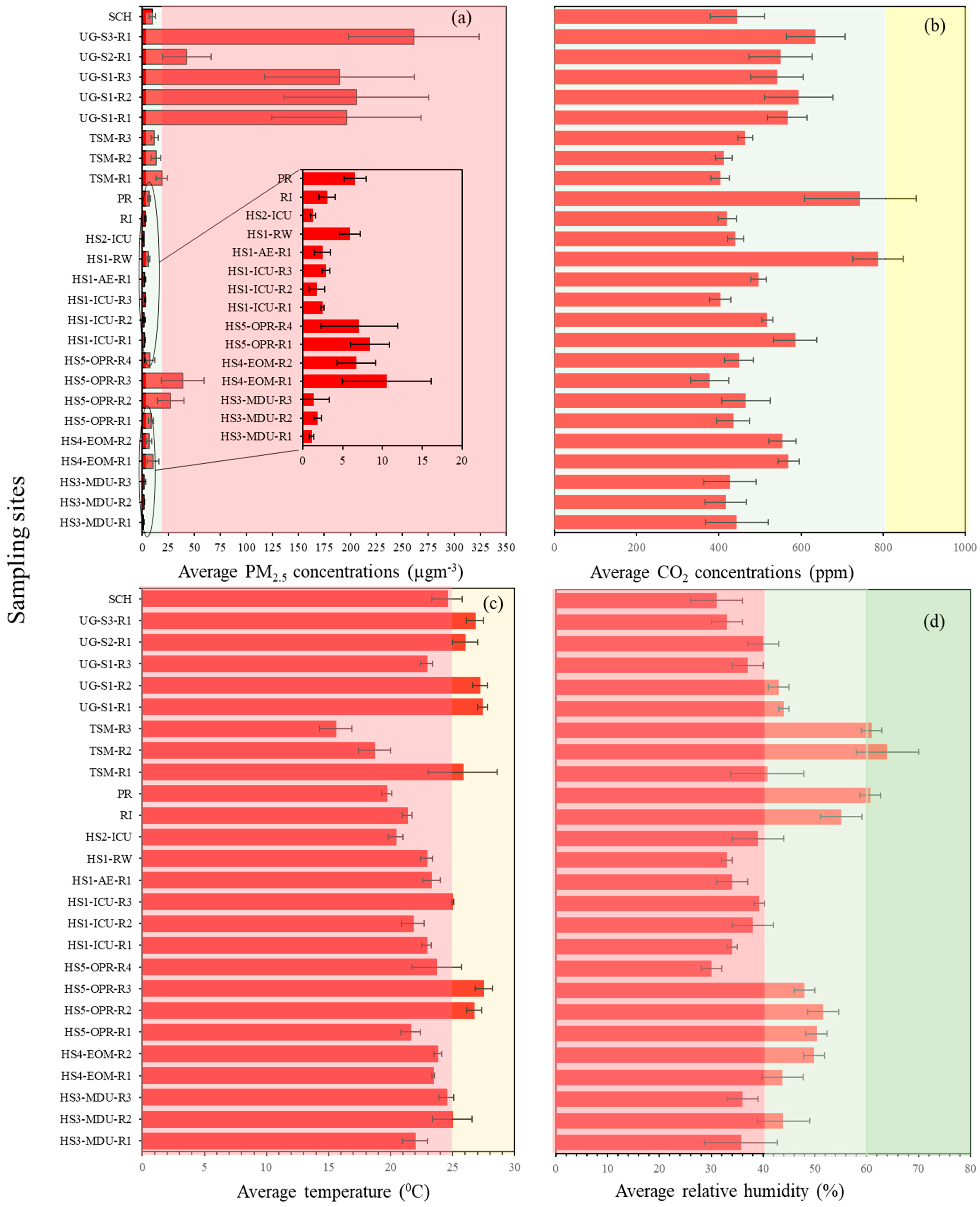
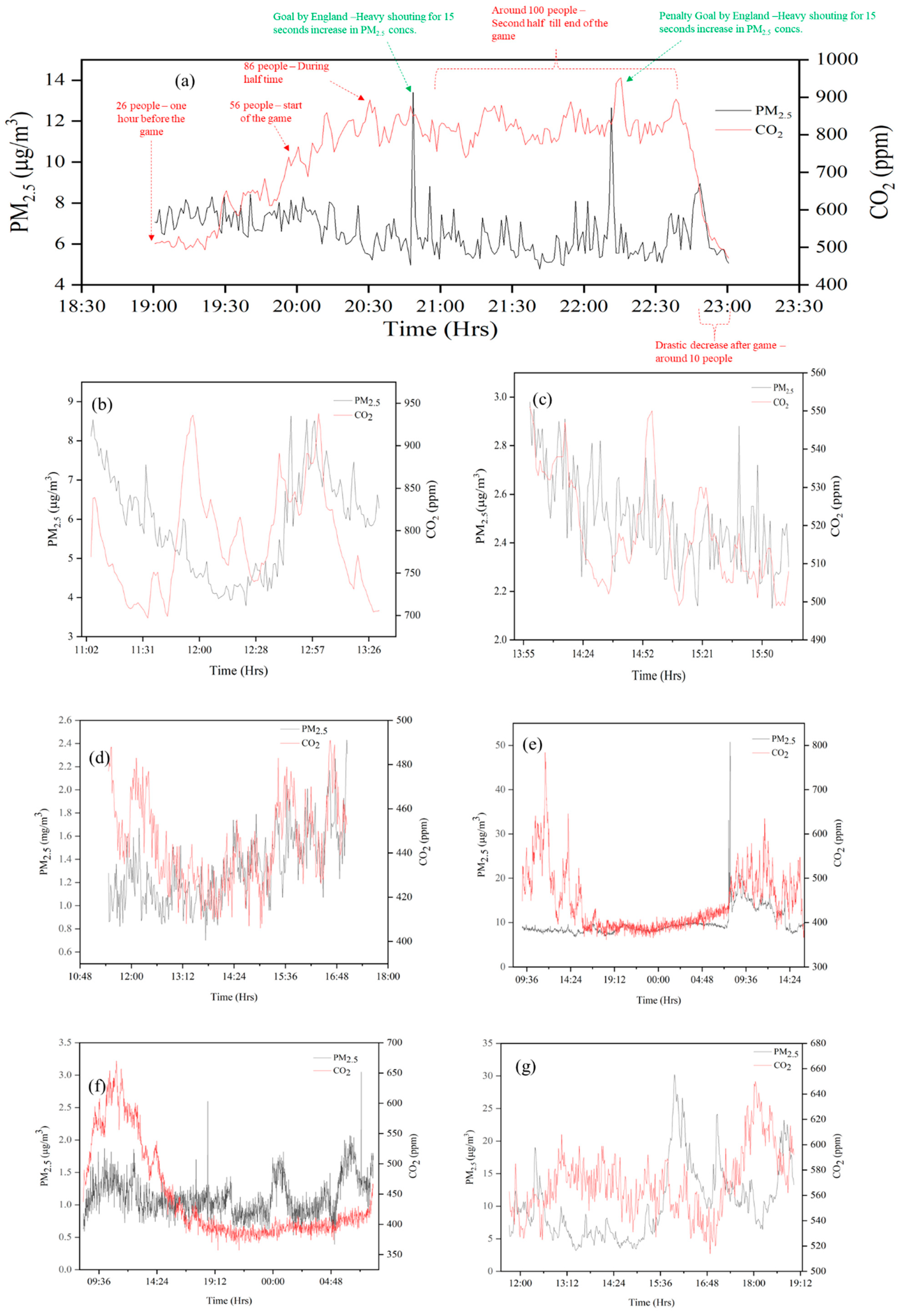
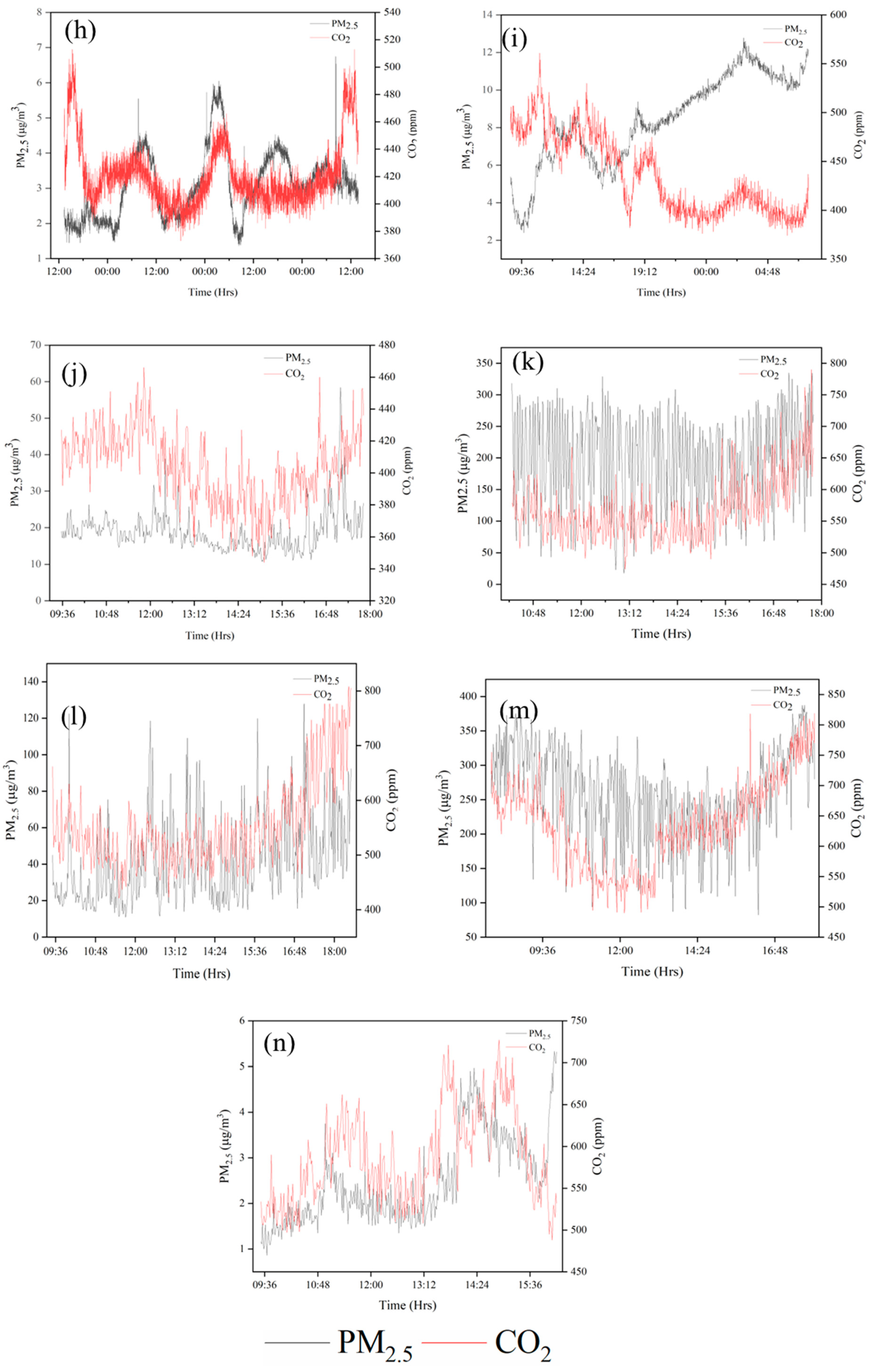
3.1. PM2.5 and CO2 Concentrations in Different Microenvironments

We monitored 14 different indoor spaces, including hospitals, train stations, a pub, a school, and a research institute; the key results such as the concentrations of PM2.5, CO2, relative humidity (RH) and temperature (mean, max, min and the standard deviation) are summarized in Figure 2 and Table S2, and the time series values are given in Figure 3. Among the hospitals, we measured a maximum CO2 concentration of 938 ppm, with the highest mean CO2 concentration of 789 ± 61 ppm recorded in the respiratory ward at Hospital number one (HS1-RW). We recorded second highest CO2 concentrations at the accident and emergency waiting rooms, and outpatient waiting room of HS1-AER—586 ± 58 ppm, HS4-EOM—570 ± 26 ppm and HS5-OPR—466 ± 59 ppm. Furthermore, the ICUs recorded 518 ± 13 ppm for HS1-ICU, 441 ± 19 ppm for HS2-ICU and 444 ± 76 ppm for the medical day unit at hospital 3. The peak concentrations recorded in the hospitals remained less than 800 ppm (except for respiratory ward in hospital 1) suggest that ventilation maybe adequate at these sampling sites. However, the high peak concentration of CO2 in the respiratory ward (HS1-RW > 800 ppm) implies that the ventilation at this site maybe suboptimal due to the full capacity of the ward due to COVID infection. At the school (SCH), train station main concourse (TSM) and research institute (RI) sites, we recorded concentrations in the range of 403 to 445 ppm. The RI sampling recorded an average concentration of 421 ± 23 ppm due to around 70% of the sampling duration taking place during the weekend when the occupancy was significantly less compared to other indoor sites. The school (SCH) sampling recorded a CO2 concentration of 445 ± 66 ppm, with a maximum concentration of 784 ppm recorded at 11:00 h, illustrating that the students’ and teachers’ breathing increased the CO2 concentrations. The lowest concentration of 403 ± 23 ppm was observed in the train station main concourse (TSM) due to the station having a solid roof but open sides, allowing enough outdoor air to circulate into the site, resulting in concentrations of CO2 close to background levels (404 ppm).
In Figure 4, we compare the mean CO2 and PM2.5 concentrations for all sites and the plot clearly demonstrates that the CO2 and PM2.5 concentrations are not correlated. The lack of correlation between these two values could be attributed to their different sources. There are also cases where they have the same source—for example, a person exhaling CO2 and PM2.5 (from their surroundings) is one source, but the CO2 and PM2.5 are produced, originally, by different mechanisms. We measured relatively low CO2 (636 ± 71 ppm) and very high PM2.5 (261 ± 62.8 μg m−3) concentrations on the underground station platform (UG-S3); the high PM2.5 concentration is attributed to the underground train emissions from the wear of train parts such as abrasions from brake shoes, brake blocks, and station sources such as escalator abrasion emissions and their resuspension due to train movements [39]. Similarly, monitoring sites near major roads—for example, HS5-OPR (38.6 ± 20.4 μg m−3), show high indoor PM levels, attributed to outdoor PM concentrations. Similar results of high PM2.5 concentrations (45.3 ± 56.4 μg m−3) (Table S2) have been observed in the indoor environment of hospitals in urban areas of Iran [40]. The air drawn into buildings for ventilation should be filtered to remove PM, since ventilation systems play a vital role in reducing indoor PM concentrations [41]. Conversely, indoor sites located at a considerable distance of about 300 to 400 m from a busy road (ICUs and MDUs of hospitals HS1, HS2 and HS3) have a PM2.5 concentration range of 1 to 3 µg m−3 with the lowest concentration of 1.1 µg m−3 and highest concentration of 2.9 µg m−3. At the school (SCH) we recorded a mean PM2.5 concentration of 10 μg m−3, which is lower than the 24 h mean concentration limit of 15 μg m−3 given by the WHO (2021). However, a surge in PM2.5 concentrations (up to 50 μg m−3) was recorded for a period of about 20 min (from 06:40 am to 07:00 am before the start of the school day), a result of the cleaning activities before school hours. The research institute had a relatively low PM2.5 concentration (3.1 ± 1 μg m−3) compared to other indoor environments (except hospital indoor sites). This is due to regular and deep cleaning meaning that there were low levels of PM2.5 available for resuspension by people. The TSM sampling recorded mean PM2.5 concentrations ranging from 13 to 19 µg m−3. However, we observed concentrations rising to 51 μg m−3 during evening peak hours (17:00 to 18:00 h). The increase in population density (due to the crowding in passenger information and train schedule board area) near the samplers, compared to other areas of the station, would have caused this increase in PM2.5 concentrations [42].
Time series data from the pub (PR); monitoring was undertaken during a major sporting event (a major football match) and the sudden spikes in PM2.5 levels were due to anthropogenic activities (such as moving and jumping) when goals were scored. These activities resuspended the particles present. It is instructive to note that the CO2 monitors did not register a similar spike and we show that CO2 and PM emission are not directly correlated (Figure 4), nevertheless CO2 gives the measure of ventilation rate which removes the pollutants from the space. Hence, the crowded sampling sites demonstrate that the occupancy is directly proportional to CO2 concentrations. However, the CO2 concentrations were less than 1000 ppm, which shows good ventilation at all the sampling sites. Similarly, the PM2.5 concentrations were relatively low and well within the DEFRA UK recommended guidelines, except for the HS5-OPR hospital close to a busy road, and the train stations (both main concourse and underground stations).
The UK’s SAGE acceptable CO2 levels of (<800 ppm) is highlighted in green and >800-ppm, highlighted in yellow, indicates poor ventilation. (c) Mean temperature recorded at all the sampling sites. The red shaded section highlights temperatures from 0 °C to 25 °C where virus viability is optimal, the yellow shaded area highlights the temperature range >25 °C to 30 °C where virus viability is moderate, and >30 °C (not included in the graph) is the temperature range with low virus viability. (d) Mean average concentrations of RH for all sampling sites. The red shaded part highlights a RH < 40% resulting in higher virus transmission risk, the pale green shaded part highlights RH of 40% to 60%, reduced transmission risk conditions, the green shaded part shows RH at 60%, which represents a potentially lower virus transmission risk, and the red shaded part with RH 0% to 40% highlights the range with increased virus transmission risk. The day of sampling and sampling duration are listed in Table 2.

3.2. Variations in Indoor Temperature and Relative Humidity

Both indoor temperature and RH are important determinants of airborne transmission and infectivity of the SARS-CoV-2 virus because these conditions affect the evaporation of the aerosol droplets. Evaporation changes the constituents within the droplets which impacts the ability of the virus to survive [43]. These conditions also influence the immune response of the recipient and therefore their susceptibility to infection [44,45].
The RH of the indoor sites is presented in Table S2. The RH values were around 40% to 64% in most of the sites located near to outdoor areas and some indoor areas, particularly those with a higher footfall. This includes outdoor sites such as the pub/restaurant (PR), research institute (RI) and the train station (TSM), and indoor sites; the underground station (UG-S1, UG-S2, UG-S3), emergency room (HS4) and outpatient room (HS5). The hospital respiratory wards (HS1-RW), ICUs (HS1-ICU and HS2-ICU), accident and emergency rooms (HS1-AER), medical day unit (HS3-MDU), school (SCH) and underground station platform (UG-S3) possess mean RH values below 40% which is optimum for maintaining the viability of the virus. Previous reports have stated that a range of RH between 40 and 60% is ideal to reduce virus transmission and SARS-CoV-2 survival [46], but it is also important to consider the influence of temperature.
Mean indoor temperatures recorded at all the sampling sites range from 15 °C to 28 °C. The lowest temperature (15.6 °C ± 1.3 °C) was recorded in the main concourse of the train station (TSM-R3), and the highest temperature (27.5 °C ± 0.7 °C) was recorded in the outpatient room (HS5). The temperature recorded in all the sampling sites, excluding the hospital indoor sites, range from 15.6 °C to 27.4 °C. Recorded temperatures in the hospital sites were in the range 20.4 °C to 27.5 °C; note that hospitals were air conditioned and ventilation units programmed to maintain a comfortable indoor temperature.
Previous modelling of the influence of temperature on the virulence of the SARS-CoV-2 virus has reported an increasing risk between 5.8 °C and 30.8 °C with case fatality risk (CFR) of 3.5 and 6.4, respectively [47]. However, the virus transmission at temperatures under 24 °C, (during the cold season) shows a negative correlation between temperature and transmission risk, though the influence of temperature on infection risk is less marked during the hot season (over 24 °C) [48]. There is also an interaction between temperature and RH. Based on a review of medical experiments on virus survival and virus transmission, virus viability and infectivity were reported to increase at a low temperature and reduced at higher temperatures. Virus survival and transmission were found to be highly efficient in a dry environment with low relative humidity, and in a wet environment with high relative humidity, and it was minimal at intermediate relative humidity [49,50]. Based on the recordings of temperatures in our study of 15.6 °C to 27.4 °C, and of RH values between 40–60%, we believe that these are low risk environments for survival and transmission of the SARS-CoV-2 virus, although the ideal temperature for reduced virus survival is between 25 °C and 30 °C.

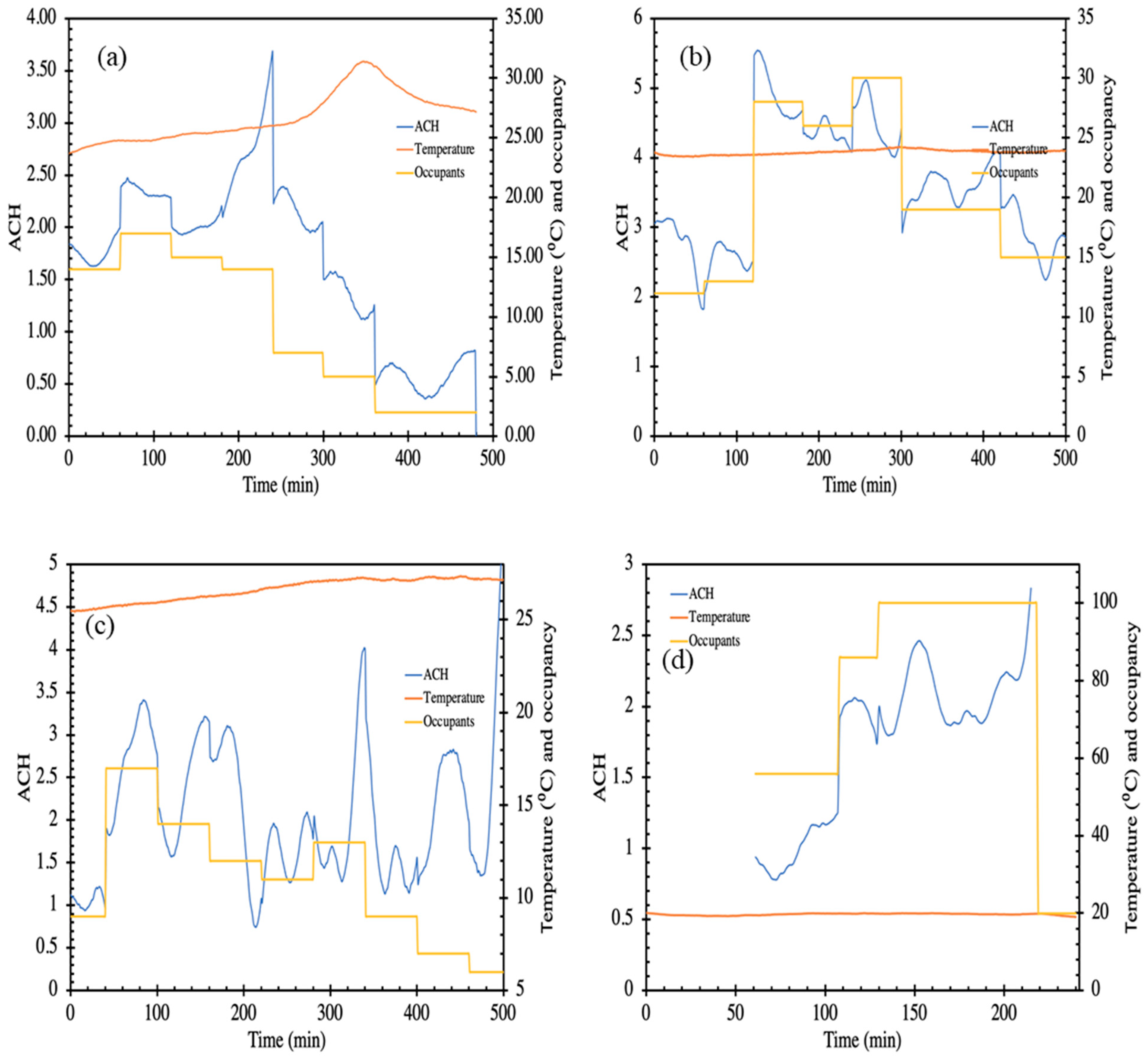
3.3. Ventilation Conditions

Figure 5 and Figure 6 present the estimated air changes and ventilation rates per person for the hospital waiting areas and pub, respectively. The air changes have been calculated only for those sites where the number of occupants were counted and recorded. Occupant data is not available for some of the sites due to limitations in permission. Figure 5a presents the measured air changes and occupancy in the medical day care unit (HS3-MDU). This space was air conditioned, and the occupancy level was high during the first half of the day (08:30 to 12:30 h). The heat and CO2 produced by the occupants are removed by the building ventilation at the rate required to maintain the temperature which, in turn, is dependent upon the heat generated internally and incoming air temperature. Qualitatively, the data presented in Figure 5b shows that a relatively constant indoor temperature was maintained, despite the variation in occupancy level, implying that the ventilation responded effectively to the changing occupancy. CO2 showed a trend similar to the occupancy—increase in occupancy also increases the CO2 level and vice versa nevertheless, at no point was the CO2 level excessively high. Data from the air-conditioned emergency waiting room (HS5-OPR) is presented in Figure 5c. CO2 concentration increases with occupancy; however, the ventilation unit was able to maintain a constant pre-set temperature (see Figure 5b), automatically adjusting the ventilation according to the occupancy. Similar trends of rise in CO2 levels with respect to the occupancy increase have been observed in experimental investigations carried out in educational buildings [51]. We want to emphasize that we estimated the ventilation rate, Q, by smoothing and differentiating a single point time series data for CO2 concentration, C(t), vs. time, t. Therefore, the caveats associated with this method are (1) the single point concentration may or may not exactly represent the global concentration in the space, (2) the errors associated with smoothing and numerical differentiation, and (3) the assumption that CO2 exhaled by the occupants are instantly mixed in the entire room. Nevertheless, this method provides a window of opportunity to examine the ventilation systems and their response to the changing occupancy. In Figure 5a, at 240 min, the occupancy decreases sharply, and so does the CO2 concentration, which the model is able to account for, but we also see a sharp peak which is an artefact of the estimation method, which could be removed by employing more sensors and obtaining an accurate measure of global CO2.
Figure 6a,b plots the ACH against the ventilation rate per person, and ventilation rate per person against the volume of the site. The ventilation rate per person in HS5-OPR was the highest (24 L person−1 s−1), followed by HS4-EOM and HS3-MDU with a ventilation rate of 19 L person−1 s−1, and the pub recorded the lowest ventilation rate of 13 L person−1 s−1. The highest site volume (1614 m3) was the pub, which was at maximum capacity, resulting in the lowest ventilation rate per person. However, ventilation rates per person were well above the guidelines (10 L person−1 s−1) as recommended by the UK government [50]. Similarly, the HS3-MDU and HS4-EOM sites have higher ventilation rates, even though the volume of the former is twice that of the latter. This could be due to lower occupancy and the location of the HS4-EOM, which was near the curbside with an automatic door opening, resulting in good fresh air exchange.
Likewise, the pub (PR) during the football match was mechanically ventilated and the doors and windows were open, providing some level of natural ventilation. The ventilation unit was able to maintain a constant indoor temperature during the match and pre-match. The CO2 concentration did not exceed 1000 ppm at any of these four sites. Hence, the ventilation per person and the air changes at all the sampling sites (HS5-OPR, HS3-MDU, HS4-EOM and PR) are well within the recommended guidelines and the ventilation settings at all sites provided sufficient air changes.

3.4. Estimation of COVID Infection Probability

We estimated the infection probability for various scenarios in which an infected individual present in a hospital waiting room speaks normally or loudly. The infected and susceptible individuals occupy the space together for the entire period and the initial concentration of virus present is assumed to be zero. We assume the following: (i) an infected individual speaking normally produces 9.4 quanta h−1; (ii) an individual speaking loudly, produces significantly more, 60.5 quanta h−1; (iii) facemasks/covering filters out 50% of the particles (Figure 7); (iv) the infected individual/speaker does not wear a mask (v) the environment is fully mixed, and a box/Wells Riley model is applicable.
We calculated the potential relative risk of infection in HS5-OPR, HS3-MDU and HS4-EOM at ventilation rates of 0.5, 1, 2, 3 and 4 ACH (Figure 7), and for different periods of exposure (between 1–8 h). The infection transmission risk values for these scenarios are tabulated in Table S3. The model estimating risk is a dynamic model and accounts for build-up of virus; the room volume influences the concentration and consequently the risk of infection. Figure 7 compares the relative risks—for the same ACH and virus released by an infected individual, the risks are different which we attribute to the room volume, and influences both the ventilation rate per person and dynamics of increasing virus. For the same ACH and number of occupants in rooms of different volumes, the ventilation rate, and the ventilation rate per person, are inherently higher for the room with larger volume, V , and consequently, the risk is expected to be higher in a room with smaller room volume and vice versa.
The volume of HS5-OPR, HS3-MDU and HS4-EOM are 640, 611 and 377 m3, respectively, and so for the same virus release rate and ACH, it is expected that the infection probability will be higher in HS4-EOM compared to HS5-OPR and HS3-MDU. The average waiting time in an emergency ward is between 2 to 4 h, and so we compared the risk of infection for a period of 4 h and at 0.5 ACH; in HS4-EOM the infection rate was estimated to be 8.5% compared to 5.1% and 5.4% at HS5-OPR and HS3-MDU, respectively.
In Figure 8, we compare the relative risks for the actual ventilation rate that were measured for different spaces. The risk of infection is very low, and this could be attributed to the higher ventilation rates, also reflected in CO2 concentrations which remained very low, indicating good ventilation levels. The probability of infection after two hours of exposure for the speaking loudly scenario (60.5 quanta h−1) (Table S5) at HS3-MDU and HS5-OPR are 1% and 1.7% at HS4-EOM (Figure S1). The infection increased to 2% and 1.5% at HS3-MDU and HS5-OPR, respectively, whereas a 0.1% decrease was found in HS4-EOM. The increase in infection transmission risk is due to the air change rate reduction in HS3-MDU (2.0 h−1) and HS5-OPR (2.72 h−1), whereas HS4-EOM has twice the air change rate (4.92 h−1) than the previous hour, which caused a 0.1% risk decrease in HS4-EOM. The infection risk for the actual ventilation rate measured for all the sites were less than the modelled scenarios, and the lowest ventilation was observed in HS3-MDU (1.7 h−1). The HS3-MDU has the second highest volume among the three hospital sites and even in the lowest ACH scenario, the infection risk is only 3% for an exposure time of 4 h. Similarly, the highest ACH (3.7 h−1) observed at HS4-EOM has the lowest room volume among these sites and the risk of infection is 2.8%. The individual, hour-based infection transmission risks for the speaking normally scenario (9.4 quanta h−1) are illustrated in Figure S2. Hence, the site (HS3-MDU) with twice the volume and half the ventilation gives the same infection risk when compared to the site (HS4-EOM) with twice the ventilation and half the volume. Once again, the results are attributed to the volume of the room and the ventilation rates, which are the main drivers of infection risk in these hospital sites.
In relation to the assumptions in the model presented here, the risk of COVID-19 infection is relatively high when the residence time of the patients/occupants is long, irrespective of the ventilation rate. We conclude that, reducing waiting times in hospitals and increasing ventilation changes in relation to the volume of the room, would significantly reduce infection risk.

4. Conclusions

In this study, we measured the PM2.5 and CO2 concentrations, RH and temperature levels, under mechanically and naturally ventilated indoor and outdoor environments of various busy, public spaces in London. In addition, the levels of CO2 in these environments have been used as a proxy to estimate the ventilation and COVID-19 transmission risk, as a result of co-exhalation of pathogen-laden particles by an infected occupant. The following conclusions are drawn:
PM2.5 concentrations in all sampling sites highlight the influence of anthropogenic PM sources. The relationship between air pollution and COVID-19 infection risk, through airborne transmission, are correlated here. We found that the total sampling area is a key driver of airborne virus transmission risk. CO2 concentration levels observed in all sites are within the SAGE UK limits for CO2 levels, except for HS1-RW (respiratory ward) and PR (Pub/Restaurant), highlighting that increasing levels of occupancy are an important contributor to CO2 levels. In addition, the room volume also plays a vital role in affecting the CO2 levels. For example, in HS1-AER, CO2 concentrations were higher than HS4-EOM and HS5-OPR, which had the same occupancy levels, but three- and five-times higher room volumes, respectively. The RH values recorded in crowded public environments such as the hospitals (emergency room (HS4) and outpatient room (HS5)), train stations (both main concourse (TSM), underground (UG)) and pub/restaurant (PR) are in the range of 44% to 64% which is optimal for reducing SARS-CoV-2 transmission risk. However, the ICUs (HS1 and HS2), Accident & Emergency room (HS1), medical day units (HS3-MDU), respiratory ward (HS1), school (SCH) and the underground platform (UG-S3) have RH measurements less than 40%, which increase the virus stability. The low RH tends to cause droplet shrinkage in the exhaled cough droplets, and prolonged suspension in ambient air, which increase the risk of airborne transmission. Conversely, higher RH increases the droplet size and increase the deposition efficiency and reducing the ambient air suspension time, thereby reducing the airborne transmission risk.
Indoor temperature values recorded at all sampling sites ranged from 15.6 °C to 27.5 °C, which is an optimal temperature range for replication of respiratory viruses in the upper airways. The indoor temperatures recorded at all sites indicate that they are high risk environments for virus spread, particularly hospital sites (HS1-RW, HS1-ICU, HS1-AER, HS4-EOM and HS5-OPR) with temperatures in the range of 22 °C to 27 °C. However, the sites such as PR, TSM, RI and hospitals near busy roadways (HS4-EOM and HS5-OPR) possess RH values in the range of 40% to 60%, reducing their viral infectivity risk. Therefore, meteorological factors such as RH and temperature are key to controlling the transmission of airborne SARS-CoV-2.
The ACH has been calculated for the mechanically ventilated sites. Exhaled CO2 and increases in temperature produced by occupants are constantly removed/corrected by ventilation systems. The trends obtained from all the environments studied indicate that, whenever the occupancy of a site increases, the CO2 levels increase and vice versa. The ventilation settings at all sampling sites were found to maintain sufficient air changes with respect to the room volume and occupancy.
The infection probability calculated using the assumed ACH values (0.5, 1, 2, 3 and 4) show that the room/space volume and occupancy plays a vital role in either reducing or increasing the infection transmission. The probability of infection calculated for 0.5 ACH (assumed low ACH value) showed twice the infection risk (HS4-EOM) of HS5-OPR and HS3-MDU whose volumes were two times higher than HS4-EOM. However, the calculated ACH value was higher in HS4-EOM followed by HS5-OPR and HS3-MDU. The higher ACH in hospital sites HS4-EOM and HS5-OPR in comparison with HS3-MDU, resulted in increased probability of infection in both the quanta emission rates of speaking loudly and normally, at 50% face mask efficiency. These results indicate that the infection transmission risk in indoor environments is correlated to the volume, ventilation conditions, and exposure time.
In order to reduce the airborne transmission of the virus, certain considerations are needed to control the thermal comfort parameters such as RH and temperature, and the provision of fresh air exchange. For example, the waiting areas of hospitals hold both undiagnosed and infected patients who may come in close contact with vulnerable patients. Our study showed that the infection probability is very low (<1%) in the hospital waiting rooms with adequate outdoor air flow, compared with the waiting room with comparatively low outdoor air influx (>1%), supporting the assertion that adequate outdoor airflow has a direct influence on reducing the risk of airborne virus transmission. Therefore, ensuring adequate fresh air exchange was found to be an effective mechanism to minimise the risk of airborne virus transmission.
This work presents a unique dataset collected in different indoor environments during the restriction periods (January 2021 to December 2021) of COVID-19, to build an understanding of their ventilation conditions and if and how that relates to the risk of airborne transmission. There is a need for similar long-term and continuous measurements at such high-occupancy sites in order to build a comparative dataset at different sites in different seasons of the year. Such a dataset would be valuable to understand the risk of airborne transmission under varying meteorological, ventilation and occupancy conditions. Additionally, it would help to appraise indoor air quality and support the validation of numerical models. Such an understanding is vital to devise mitigation strategies for controlling airborne transmission risks for viruses such as COVID-19.

Supplementary Materials

The following supporting information can be downloaded at: https://www.mdpi.com/article/10.3390/atmos13122067/s1, Figure S1: Probability of COVID-19 transmission (%) for the scenario of speaking loudly at (a) Hour one; (b) Hour 2; (c) Hour 3; (d) Hour 4; (e) Hour 5; (f) Hour 6; (g) Hour 7 and (h) Hour 8 where both infected/uninfected occupants wore face masks with 50% efficiency versus time; Figure S2: Probability of COVID-19 transmission (%) for the scenario of speaking normally at (a) Hour one; (b) Hour 2; (c) Hour 3; (d) Hour 4; (e) Hour 5; (f) Hour 6; (g) Hour 7 and (h) Hour 8 where both infected/uninfected occupants wore face masks with 50% efficiency versus time; Figure S3: Relative probability of infection transmission using HS5-OPR as the base case scenario with respect to HS4-EOM and HS3-MDU; Figure S4: Mean ACH values for mechanically ventilated indoor environments against Size/Occupancy for HS5-OPR, HS3-MDU, HS4-EOM and PR. Table S1: List of sampling days and the relevant number of recorded cases and the infection prevalence (%) calculated against the London population for each day and the cumulative days since 11 February 2020. (Ref: https://coronavirus.data.gov.uk/details/cases?areaType=region&areaName=London, accessed on 10 November 2022); Table S2. Brief description of sampling sites, site codes, description of the site, and the total sampled hours. All the sampling sites have been anonymised for confidentiality reasons; Table S3: Probability of infection transmission (%) using the assumed ventilation values (ACH) such as 0.5, 1, 2, 3 and 4 for the two scenarios: speaking loudly (SL-60.5 quanta h−1) and speaking normal (SN-9.4 quanta h−1) for HS5-OPR, HS4-EOM and HS3-MDU; Table S4. Probability of infection transmission (%) using the calculated ventilation value (ACH) for the two scenarios: speaking loudly (SL-60.5 quanta h−1) and speaking normal (SN-9.4 quanta h−1) for HS5-OPR, HS4-EOM and HS3-MDU.

Author Contributions

Conceptualization, P.K.; methodology, P.K., G.K. and R.K.B.; validation, G.K. and R.K.B.; formal analysis, G.K., R.K.B. and P.K.; investigation, S.M., I.M.A., A.E.P., E.R., H.A.-W., S.S., P.B., C.D., C.C.P. and K.F.C.; data curation, P.K., G.K. and R.K.B.; writing—original draft preparation, P.K., G.K. and R.K.B.; writing—review and editing, P.K., G.K., R.K.B., S.M., I.M.A., A.E.P., E.R., H.A.-W., S.S., P.B., C.D., C.C.P., F.F. and K.F.C.; visualization, P.K., G.K. and R.K.B.; supervision, P.K.; project administration, P.K., G.K. and C.D.; funding acquisition, P.K., C.C.P. and K.F.C. All authors have read and agreed to the published version of the manuscript.

Funding

This work has been carried out as a part of the Engineering and Physical Research Council (EPSRC) funded COVAIR (EP/V052462/1; Is SARS-CoV-2 airborne and does it interact with particle pollutants?) project under the COVID-19 call. R.K.B. acknowledges support from Leverhulme Trust.

Institutional Review Board Statement

Not applicable.

Informed Consent Statement

Not applicable.

Data Availability Statement

Not applicable.

Acknowledgments

The authors thank the authorities of the hospitals, train stations, schools, research institutes and pub/restaurants for granting permissions to sample on their premises, and for their help in setting up the instruments to carry out the air sampling. The views presented in this paper are those of the authors, except otherwise indicated. The authors do not certify, endorse, or recommend any trade names or commercial products referred to in this article.

Conflicts of Interest

The authors declare no conflict of interest.

References

  1. Lednicky, J.A.; Lauzard, M.; Fan, Z.H.; Jutla, A.; Tilly, T.B.; Gangwar, M.; Usmani, M.; Shankar, S.N.; Mohamed, K.; Eiguren-Fernandez, A.; et al. Viable SARS-CoV-2 in the air of a hospital room with COVID-19 patients. Int. J. Infect. Dis. 2020, 100, 476–482. [Google Scholar] [CrossRef] [PubMed]
  2. Li, Q.; Guan, X.; Wu, P.; Wang, X.; Zhou, L.; Tong, Y.; Ren, R.; Leung, K.S.M.; Lau, E.H.Y.; Wong, J.Y.; et al. Early Transmission Dynamics in Wuhan, China, of Novel Coronavirus–Infected Pneumonia. N. Engl. J. Med. 2020, 382, 1199–1207. [Google Scholar] [CrossRef] [PubMed]
  3. Li, C.; Tang, H. Comparison of COVID-19 infection risks through aerosol transmission in supermarkets and small shops. Sustain. Cities Soc. 2022, 76, 103424. [Google Scholar] [CrossRef] [PubMed]
  4. Miranda, M.T.; Romero, P.; Valero-Amaro, V.; Arranz, J.I.; Montero, I. Ventilation conditions and their influence on thermal comfort in examination classrooms in times of COVID-19. A case study in a Spanish area with Mediterranean climate. Int. J. Hyg. Environ. Health 2022, 240, 113910. [Google Scholar] [CrossRef] [PubMed]
  5. Kumar, P.; Omidvarborna, H.; Tiwari, A.; Morawska, L. The nexus between in-car aerosol concentrations, ventilation and the risk of respiratory infection. Environ. Int. 2021, 157, 106814. [Google Scholar] [CrossRef]
  6. Stabile, L.; Buonanno, G.; Frattolillo, A.; Dell’Isola, M. The effect of the ventilation retrofit in a school on CO2, airborne particles, and energy consumptions. Build. Environ. 2019, 156, 1–11. [Google Scholar] [CrossRef]
  7. Di Gilio, A.; Palmisani, J.; Pulimeno, M.; Cerino, F.; Cacace, M.; Miani, A.; de Gennaro, G. CO2 concentration monitoring inside educational buildings as a strategic tool to reduce the risk of SARS-CoV-2 airborne transmission. Environ. Res. 2021, 202, 111560. [Google Scholar] [CrossRef]
  8. Villanueva, F.; Notario, A.; Cabañas, B.; Martín, P.; Salgado, S.; Gabriel, M.F. Assessment of CO2 and aerosol (PM2.5, PM10, UFP) concentrations during the reopening of schools in the COVID-19 pandemic: The case of a metropolitan area in Central-Southern Spain. Environ. Res. 2021, 197, 111092. [Google Scholar] [CrossRef]
  9. Schade, W.; Reimer, V.; Seipenbusch, M.; Willer, U. Experimental investigation of aerosol and CO2 dispersion for evaluation of COVID-19 infection risk in a concert hall. Int. J. Environ. Res. Public Health 2021, 18, 3037. [Google Scholar] [CrossRef]
  10. Bazant, M.Z.; Kodio, O.; Cohen, A.E.; Khan, K.; Gu, Z.; Bush, J.W.M. Monitoring carbon dioxide to quantify the risk of indoor airborne transmission of COVID-19. Flow 2021, 1, 1–18. [Google Scholar] [CrossRef]
  11. Deol, A.K.; Scarponi, D.; Beckwith, P.; Yates, T.A.; Karat, A.S.; Yan, A.W.C.; Baisley, K.S.; Grant, A.D.; White, R.G.; McCreesh, N. Estimating ventilation rates in rooms with varying occupancy levels: Relevance for reducing transmission risk of airborne pathogens. PLoS ONE 2021, 16, e0253096. [Google Scholar] [CrossRef] [PubMed]
  12. Pavilonis, B.; Ierardi, A.M.; Levine, L.; Mirer, F.; Kelvin, E.A. Estimating aerosol transmission risk of SARS-CoV-2 in New York City public schools during reopening. Environ. Res. 2021, 195, 110805. [Google Scholar] [CrossRef] [PubMed]
  13. Holshue, M.L.; DeBolt, C.; Lindquist, S.; Lofy, K.H.; Wiesman, J.; Bruce, H.; Spitters, C.; Ericson, K.; Wilkerson, S.; Tural, A.; et al. First Case of 2019 Novel Coronavirus in the United States. N. Engl. J. Med. 2020, 382, 929–936. [Google Scholar] [CrossRef]
  14. Khanna, C.R.; Cicinelli, M.V.; Gilbert, S.S.; Honavar, G.S.; Gudlavalleti, V.S.M. COVID-19 pandemic: Lessons learned and future directions. Indian J. Ophthalmol. 2020, 68, 703–710. [Google Scholar] [CrossRef] [PubMed]
  15. Al Huraimel, K.; Alhosani, M.; Kunhabdulla, S.; Stietiya, M.H. SARS-CoV-2 in the environment: Modes of transmission, early detection and potential role of pollutions. Sci. Total Environ. 2020, 744, 140946. [Google Scholar] [CrossRef] [PubMed]
  16. Kumar, P.; Hama, S.; Omidvarborna, H.; Sharma, A.; Sahani, J.; Abhijith, K.V.; Debele, S.E.; Zavala-Reyes, J.C.; Barwise, Y.; Tiwari, A. Temporary reduction in fine particulate matter due to ‘anthropogenic emissions switch-off’ during COVID-19 lockdown in Indian cities. Sustain. Cities Soc. 2020, 62, 102382. [Google Scholar] [CrossRef]
  17. Enyoh, C.E.; Verla, A.W.; Qingyue, W.; Yadav, D.K.; Hossain Chowdhury, M.; Isiuku, B.O.; Chowdhury, T.; Ibe, F.C.; Verla, E.N.; Maduka, T.O. Indirect Exposure to Novel Coronavirus (SARS-CoV-2): An Overview of Current Knowledge. J. Teknol. Lab. 2020, 9, 67–77. [Google Scholar] [CrossRef]
  18. Kampf, G.; Todt, D.; Pfaender, S.; Steinmann, E. Persistence of coronaviruses on inanimate surfaces and their inactivation with biocidal agents. J. Hosp. Infect. 2020, 104, 246–251. [Google Scholar] [CrossRef] [Green Version]
  19. Setti, L.; Passarini, F.; De Gennaro, G.; Barbieri, P.; Perrone, M.G.; Borelli, M.; Palmisani, J.; Di Gilio, A.; Piscitelli, P.; Miani, A. Airborne transmission route of COVID-19: Why 2 meters/6 feet of interpersonal distance could not be enough. Int. J. Environ. Res. Public Health 2020, 17, 2932. [Google Scholar] [CrossRef] [Green Version]
  20. Jayaweera, M.; Perera, H.; Gunawardana, B.; Manatunge, J. Transmission of COVID-19 virus by droplets and aerosols: A critical review on the unresolved dichotomy. Environ. Res. 2020, 188, 109819. [Google Scholar] [CrossRef]
  21. Morawska, L.; Cao, J. Airborne transmission of SARS-CoV-2: The world should face the reality. Environ. Int. 2020, 139, 105730. [Google Scholar] [CrossRef] [PubMed]
  22. Wang, D.; Hu, B.; Hu, C.; Zhu, F.; Liu, X.; Zhang, J.; Wang, B.; Xiang, H.; Cheng, Z.; Xiong, Y.; et al. Clinical Characteristics of 138 Hospitalized Patients with 2019 Novel Coronavirus-Infected Pneumonia in Wuhan, China. J. Am. Med. Assoc. 2020, 323, 1061–1069. [Google Scholar] [CrossRef] [PubMed]
  23. Chia, P.Y.; Coleman, K.K.; Tan, Y.K.; Ong, S.W.X.; Gum, M.; Lau, S.K.; Lim, X.F.; Lim, A.S.; Sutjipto, S.; Lee, P.H.; et al. Detection of air and surface contamination by SARS-CoV-2 in hospital rooms of infected patients. Nat. Commun. 2020, 11, 2800. [Google Scholar] [CrossRef] [PubMed]
  24. Zhou, A.J.; Otter, J.A.; Price, J.R.; Cimpeanu, C.; Garcia, M.; Kinross, J.; Boshier, P.R.; Mason, S.; Bolt, F.; Alison, H.; et al. Investigating SARS-CoV-2 surface and air contamination in an acute healthcare setting during the peak of the COVID-19 pandemic in London. medRxiv 2020. [Google Scholar] [CrossRef]
  25. Bulfone, T.C.; Malekinejad, M.; Rutherford, G.W.; Razani, N. Outdoor Transmission of SARS-CoV-2 and Other Respiratory Viruses: A Systematic Review. J. Infect. Dis. 2021, 223, 550–561. [Google Scholar] [CrossRef]
  26. Stabile, L.; Pacitto, A.; Mikszewski, A.; Morawska, L.; Buonanno, G. Ventilation procedures to minimize the airborne transmission of viruses in classrooms. Build. Environ. 2021, 202, 108042. [Google Scholar] [CrossRef]
  27. Rodríguez, M.; Llanos Palop, M.; Seseña, S.; Rodríguez, A. Are the Portable Air Cleaners (PAC) really effective to terminate airborne SARS-CoV-2? Sci. Total Environ. 2021, 785, 147300. [Google Scholar] [CrossRef]
  28. Zhu, S.; Jenkins, S.; Addo, K.; Heidarinejad, M.; Romo, S.A.; Layne, A.; Ehizibolo, J.; Dalgo, D.; Mattise, N.W.; Hong, F.; et al. Ventilation and laboratory confirmed acute respiratory infection (ARI) rates in college residence halls in College Park, Maryland. Environ. Int. 2020, 137, 105537. [Google Scholar] [CrossRef]
  29. Kumar, P.; Rawat, N.; Tiwari, A. Micro-characteristics of a naturally ventilated classroom air quality under varying air purifier placements. Environ. Res. 2022, in press. [Google Scholar] [CrossRef]
  30. Nor, N.S.M.; Yip, C.W.; Ibrahim, N.; Jaafar, M.H.; Rashid, Z.Z.; Mustafa, N.; Hamid, A.H.H.; Chandru, K.; Latif, M.T.; Saw, P.E.; et al. Particulate matter (PM2.5) as a potential SARS-CoV-2 carrier. Sci. Rep. 2021, 11, 2508. [Google Scholar] [CrossRef]
  31. Ahlawat, A.; Wiedensohler, A.; Mishra, S.K. An overview on the role of relative humidity in airborne transmission of SARS-CoV-2 in indoor environments. Aerosol Air Qual. Res. 2020, 20, 1856–1861. [Google Scholar] [CrossRef]
  32. Bhagat, R.; Davies Wykes, M.; Dalziel, S.; Linden, P. Effects of ventilation on the indoor spread of COVID-19. J. Fluid Mech. 2020, 903, F1. [Google Scholar] [CrossRef] [PubMed]
  33. Woodward, H.; de Kreij, R.J.B.; Kruger, E.S.; Fan, S.; Tiwari, A.; Hama, S.; Noel, S.; Wykes, M.S.D.; Kumar, P.; Linden, P.F. An evaluation of the risk of airborne transmission of COVID-19 on an inter-city train carriage. Indoor Air 2022, 32, e13121. [Google Scholar] [CrossRef] [PubMed]
  34. Buonanno, G.; Stabile, L.; Morawska, L. Estimation of airborne viral emission: Quanta emission rate of SARS-CoV-2 for infection risk assessment. Environ. Int. 2020, 141, 105794. [Google Scholar] [CrossRef]
  35. Miller, S.L.; Nazaroff, W.W.; Jimenez, J.L.; Boerstra, A.; Buonanno, G.; Dancer, S.J.; Kurnitski, J.; Marr, L.C.; Morawska, L.; Noakes, C. Transmission of SARS-CoV-2 by inhalation of respiratory aerosol in the Skagit Valley Chorale superspreading event. Indoor Air 2021, 31, 314–323. [Google Scholar] [CrossRef]
  36. Batterman, S. Review and extension of CO2-based methods to determine ventilation rates with application to school classrooms. Int. J. Environ. Res. Public Health 2017, 14, 145. [Google Scholar] [CrossRef] [Green Version]
  37. Kappelt, N.; Russell, H.S.; Kwiatkowski, S.; Afshari, A.; Johnson, M.S. Correlation of Respiratory Aerosols with Metabolic Carbon Dioxide. 2021. Available online: https://www.researchsquare.com/article/rs-490702/v1 (accessed on 20 July 2021).
  38. Pawar, S.; Stanam, A.; Chaudhari, M.; Rayudu, D. Effects of temperature on COVID-19 transmission. medRxiv 2020. [Google Scholar] [CrossRef] [Green Version]
  39. Smith, J.D.; Barratt, B.M.; Fuller, G.W.; Kelly, F.J.; Loxham, M.; Nicolosi, E.; Priestman, M.; Tremper, A.H.; Green, D.C. PM2.5 on the London Underground. Environ. Int. 2020, 134, 105188. [Google Scholar] [CrossRef] [PubMed]
  40. Mohammadyan, M.; Keyvani, S.; Bahrami, A.; Yetilmezsoy, K.; Heibati, B.; Pollitt, K.J.G. Assessment of indoor air pollution exposure in urban hospital microenvironments. Air Qual. Atmos. Health 2019, 12, 151–159. [Google Scholar] [CrossRef]
  41. Morawska, L.; Jamriska, M.; Guo, H.; Jayaratne, E.R.; Cao, M.; Summerville, S. Variation in indoor particle number and PM2.5 concentrations in a radio station surrounded by busy roads before and after an upgrade of the HVAC system. Build. Environ. 2009, 44, 76–84. [Google Scholar] [CrossRef]
  42. Zhao, X.; Zhou, W.; Han, L.; Locke, D. Spatiotemporal variation in PM2.5 concentrations and their relationship with socioeconomic factors in China’s major cities. Environ. Int. 2019, 133, 105145. [Google Scholar] [CrossRef] [PubMed]
  43. Noti, J.D.; Blachere, F.M.; McMillen, C.M.; Lindsley, W.G.; Kashon, M.L.; Slaughter, D.R.; Beezhold, D.H. High Humidity Leads to Loss of Infectious Influenza Virus from Simulated Coughs. PLoS ONE 2013, 8, e57485. [Google Scholar] [CrossRef] [PubMed]
  44. Nottmeyer, L.; Armstrong, B.; Lowe, R.; Abbott, S.; Meakin, S.; O’Reilly, K. The association of COVID-19 incidence with temperature, humidity, and UV radiation-A global multi-city analysis. Sci. Total Environ. 2022, 854, 158636. [Google Scholar] [CrossRef] [PubMed]
  45. Smither, S.J.; Eastaugh, L.S.; Findlay, J.S.; Lever, M.S. Experimental aerosol survival of SARS-CoV-2 in artificial saliva and tissue culture media at medium and high humidity. Emerg. Microbes Infect. 2020, 9, 1415–1417. [Google Scholar] [CrossRef]
  46. Thornton, G.M.; Fleck, B.A.; Dandnayak, D.; Kroeker, E.; Zhong, L.; Hartling, L. The impact of heating, ventilation, and air conditioning (HVAC) design features on the transmission of viruses, including the 2019 novel coronavirus (COVID-19): A systematic review of humidity. PLoS ONE 2022, 17, e0275654. [Google Scholar] [CrossRef] [PubMed]
  47. Yamasaki, L.; Murayama, H.; Hashizume, M. The impact of temperature on the transmissibility and virulence of COVID-19 in Tokyo, Japan. Sci. Rep. 2021, 11, 24477. [Google Scholar] [CrossRef]
  48. Mao, N.; Zhang, D.; Li, Y.; Li, Y.; Li, J.; Zhao, L. How do temperature, humidity, and air saturation state affect the COVID-19 transmission risk? Environ. Sci. Pollut. Res. 2022, 1–15. [Google Scholar] [CrossRef]
  49. Guo, L.; Yang, Z.; Zhang, L.; Wang, S.; Bai, T.; Xiang, Y.; Long, E. Systematic review of the effects of environmental factors on virus inactivation: Implications for coronavirus disease 2019. Int. J. Environ. Sci. Technol. 2021, 18, 2865–2878. [Google Scholar] [CrossRef]
  50. Aganovic, A.; Bi, Y.; Cao, G.; Drangsholt, F.; Kurnitski, J. Estimating the impact of indoor relative humidity on SARS-CoV-2 airborne transmission risk using a new modification of the Wells-Riley model. Build. Environ. 2021, 205, 108278. [Google Scholar] [CrossRef]
  51. Zivelonghi, A.; Lai, M. Mitigating aerosol infection risk in school buildings: The role of natural ventilation, volume, occupancy, and CO2 monitoring. Build. Environ. 2021, 204, 108139. [Google Scholar] [CrossRef]
Figure 1. Schematic representation of raw and smoothened CO2 data in (a) Hospital medical day unit (HS3-MDU); (b) Hospital emergency and outpatient waiting room (HS4-EOM); (c) Hospital outpatient waiting room (HS5-OPR); (d) Pub/restaurant (PR).
Atmosphere 13 02067 g001
Figure 2. (a) Mean PM2.5 concentrations at all sampling sites. The green shaded part shows the DEFRA UK standard acceptable levels for 24 h average exposure to 15 µg m−3 for PM2.5 concentrations. (b) Mean CO2 concentrations at all the sampling sites. (c) Mean temperature recorded at all the sampling sites. The red shaded section highlights temperatures from 0 °C to 25 °C where virus viability is optimal, the yellow shaded area highlights the temperature range >25 °C to 30 °C where virus viability is moderate, and >30 °C (not included in the graph) is the temperature range with low virus viability. (d) Mean average concentrations of RH for all sampling sites. The red shaded part highlights a RH < 40% resulting in higher virus transmission risk, the pale green shaded part highlights RH of 40% to 60%, reduced transmission risk conditions, the green shaded part shows RH at 60%, which represents a potentially lower virus transmission risk, and the red shaded part with RH 0% to 40% highlights the range with increased virus transmission risk.
Atmosphere 13 02067 g002
Figure 3. Time series of PM2.5 and CO2 at all sampling sites (a) PR; (b) HS1-RW; (c) HS1-ICU; (d) HS2-ICU; (e) SCH; (f) HS3-MDU; (g) HS4-EOM; (h) RI; (i) HS5-OPR; (j) TSM; (k) UG-S1; (l) UG-S2; (m) UG-S3; (n) HS1-AER. As an example, the concentration values of the first sampling run are shown in the figure.
Atmosphere 13 02067 g003aAtmosphere 13 02067 g003b
Figure 4. Comparison of mean CO2 and PM2.5 concentrations from all sites to highlight the lack of correlation between the sources of CO2 and PM2.5.
Atmosphere 13 02067 g004
Figure 5. Schematic representation of air changes per hour (ACH), temperature and number of occupants in (a) HS3-MDU; (b) HS4-EOM; (c) HS5-OPR; (d) PR. where the primary axes depicting calculated air change per hour (ACH) plotted against time during the occupancy period. The secondary axis shows the temperature and occupancy.
Atmosphere 13 02067 g005
Figure 6. (a) Mean ACH values for mechanically ventilated indoor environments against ventilation rate per person for HS5-OPR, HS3-MDU, HS4-EOM and PR. (b) Ventilation rate plotted against volume in indoor environments (HS5-OPR, HS3-MDU, HS4-EOM, PR) to show the influence of the room volume on ventilation rate per person.
Atmosphere 13 02067 g006
Figure 7. Probability of COVID-19 transmission (%) for the speaking loudly scenario (SL) and speaking normally (SN) by using the assumed five different ACH values such as 0.5, 1, 2, 3 and 4 to estimate the effect of ACH on the infection transmission for (a) HS5-OPR; (b) HS3-MDU and (c) HS4-EOM.
Atmosphere 13 02067 g007
Figure 8. Probability of COVID-19 transmission (%) for the speaking loudly scenario (SL) and for the scenario of speaking normally (SN) where both infected/uninfected occupants wore face masks with 50% efficiency versus time.
Atmosphere 13 02067 g008
Table 1. Summary of previous studies monitoring PM2.5 and/or CO2 concentrations for assessing the air change rates, ventilation settings and infection transmission of COVID-19.
Type of EnvironmentPollutantsDescriptionReference
Supermarkets and small shopsCO2The average infection risk in supermarkets is higher than small shops (p-value < 0.001). Infection risks are higher for staff working with infected staff compared to customers.[3]
Education centersCO2The maximum CO2 concentration value recorded in one of the tests was 808 ppm, which is the limit for category IDA 2 buildings (including educational establishments), which was not exceeded. The report recommended that windows should be open when outside temperatures are mild.[4]
In carPM2.5 and CO2The probability of transmission from an infected person was found to be lower when the windows were open, the risk of infection increased 2-fold in a windows closed-Air conditioning scenario, and 10-fold in a windows closed-recirculation scenario.[5]
ClassroomsCO2A mass balance approach was used to quantify the ability of both mechanical ventilation and ad hoc airing to mitigate airborne transmission. The mechanically ventilated classrooms required a control unit in order to check the air exchange rate and set the corresponding constant fresh flow rate. Whereas naturally ventilated classrooms needed to have manual airing cycles to increase the air exchange rate, which, in turn, reduced the probability of SARS-CoV-2 infection transmission.[6]
ClassroomsCO2The CO2 monitoring in real-time helps to formulate tailored ventilation protocol to devise effective air exchanges and prevent SARS-CoV-2 transmission.[7]
Educational buildingsCO2, PM2.5, PM10 and UFPThe preschool rooms registered better ventilation conditions, while secondary classrooms exhibited the highest peak and average CO2 concentrations.[8]
Concert halldi-ethylhexyl-sebacate aerosols (0.3 µm) (DEHS) and CO2The results show that a performer who is a potential emitter of aerosols with 0.3 µm diameter at 1.5 m distance would be carried up to the ceiling by the fresh air ventilation system with a vertical air flow of 0.05 m/s. Under these conditions, aerosol and CO2 concentrations did increase significantly in the concert hall. Audiences can wear facemasks to protect against longer range transport of small and large particles.[9]
Lecture HallsCO2CO2 in a well-mixed space acts as a passive scalar by tracking the ambient flow conditions and is removed only through exchange with outdoor air. The use of face masks reduces the ratio of aerosol-borne pathogen to CO2 concentration dramatically, and therefore reduces the risk of indoor transmission.[10]
Primary health clinicCO2Improved ventilation not only potentially reduces COVID-19 deaths, but also reduces the high numbers of deaths that occur from other airborne infectious diseases such as tuberculosis.[11]
ClassroomsCO2Transmission probabilities are lower in older school buildings and lower-income neighborhoods due to the greater outdoor airflow associated with older, non-renovated buildings that are poorly insulated.[12]
Table 2. Description of sampling site, the total number of sampling hours and the number of samples collected and the type of ventilation (NPV—Negative pressure ventilation; MV—Mechanical Ventilation, NV—Natural Ventilation) at all the sampling sites. All the sampling sites have been anonymized for confidentiality reasons.
Sampling Site (Code)Number of Samples (n)Sampling DurationTotal Hours Sampled (h)Type of VentilationOccupants
Start TimeEnd Time
Hospital number 1 Respiratory ward (HS1-RW)14911:03:4513:31:452.28NPV4 patients occupying in a ward with 6 beds
Hospital number 1 Intensive Care Unit (HS1-ICU)12613:58:1716:03:172.05NPVNA
147313:04:4413:37:4424.33NPVNA
36711:45:4017:52:406:07NPVNA
Hospital number 1 Accident and Emergency ward (HS1-AER)40109:30:5716:11:576:41MVAround 5–14 during (09:30 to 16:30 h)
Hospital number 2 Intensive Care Unit (HS2-ICU)33511:2817:03:015.35NPVNA
School (SCH)185808:58:5115:56:5130.57MVNA
Hospital 3 Medical Day Unit (HS3-MDU)145408:04:0908:18:0924.14MVAround 12–15 during (08:30 to 12:30 h)
140608:48:3408:14:3423:36MVAround 12–15 during (08:30 to 12:30 h)
145209:30:0609:42:0624:12MVAround 08–16 during (09:30 to 13:00 h)
Hospital 4 Emergency/Outpatient Room (HS4-EOM)43911:42:4319:01:437.19MVAround 15–20 during (09:00 to 18:00 h)
52009:42:0918:22:098.40MVAround 15–20 during (09:00 to 18:00 h)
Research Institute (RI)435713:15:3913:52:3972:37MVAround 10 during (09:00 to 17:00 h)
Hospital 5 Outpatient Ward (HS5-OPR)139708:42:4307:59:4323.20MVAround 10–12 during (08:30 to 16:00 h)
140209:05:5108:27:5123.38MVAround 10–12 during (08:30 to 16:00 h)
137509:30:4308:25:4322:55MVAround 3–13 during (09:30 to 17:00 h)
144109:35:4809:36:4824:01MVAround 5–14 during (09:35 to 17:00 h)
Pub/Restaurant (PR)25418:46:3323:00:334.14MVAround 80 to 100 during (18:00 to 23:00 h)
Train station main concourse (TSM)49709:31:4517:49:458.18NVCommuters to national rail and tube
54609:20:2218:26:229:06NVCommuters to national rail and tube
42409:15:3916:19:397:04NVCommuters to national rail and tube
Underground Site1 (UG-S1)45310:15:5117:48:517:33MVCommuters to national rail and other tube stations
55609:15:1018:31:109:16MVCommuters to national rail and other tube stations
Underground Site1 (UG-S2)44009:50:0717:10:077:20MVCommuters to national rail and other tube station
54109:30:2618:31:269:01NVCommuters to national rail and other tube station
Underground Site3 (UG-S3)60308:00:0818:03:0810:03MVCommuters to national rail and other tube station
Publisher’s Note: MDPI stays neutral with regard to jurisdictional claims in published maps and institutional affiliations.

