
Improvement in Predicting the Post-Cracking Tensile Behavior of Ultra-High Performance Cementitious Composites Based on Fiber Orientation Distribution


Abstract
:1. Introduction
2. Experimental Program
2.1. Materials and Mix Design
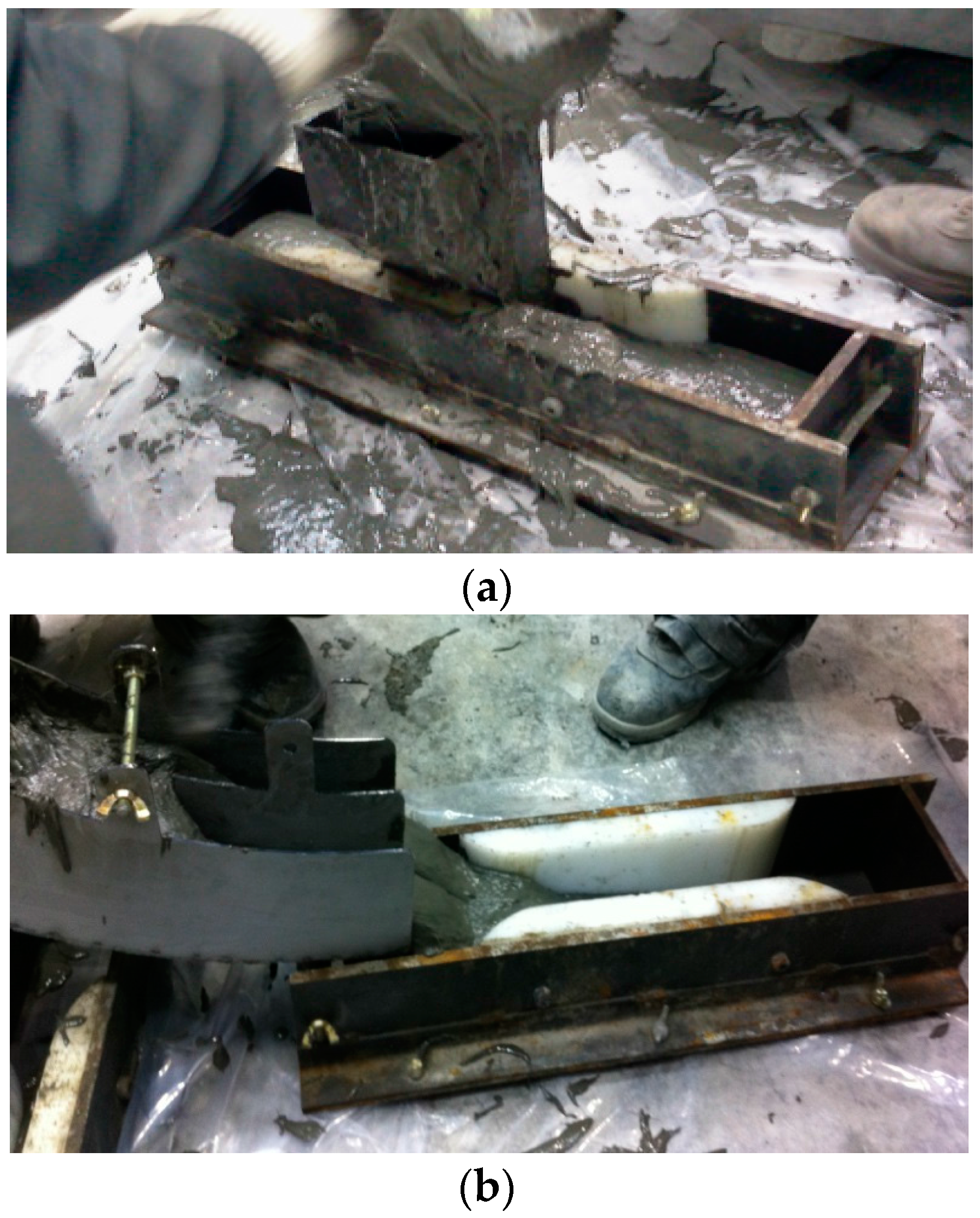
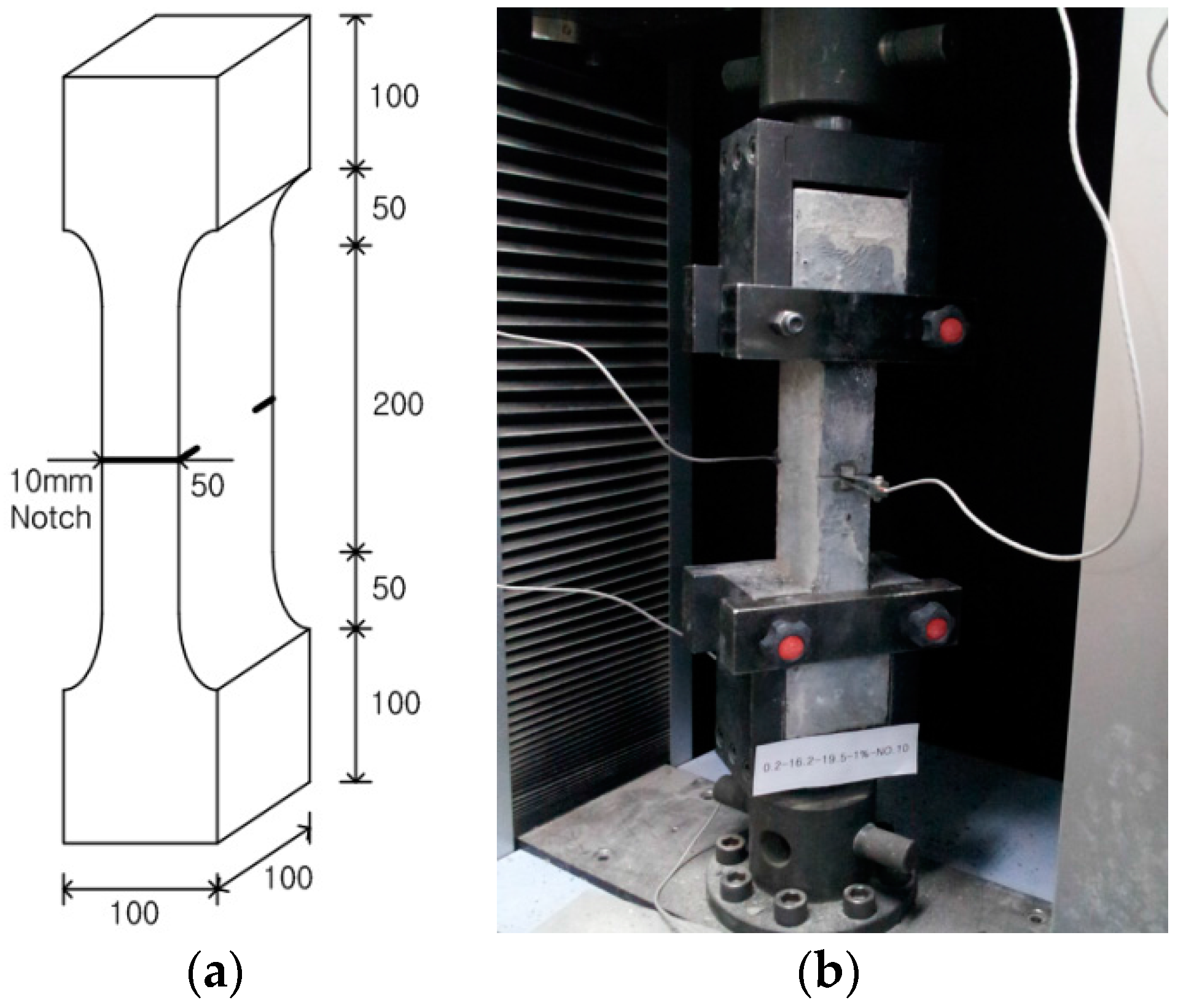
2.2. Specimen Preparation and Experiment
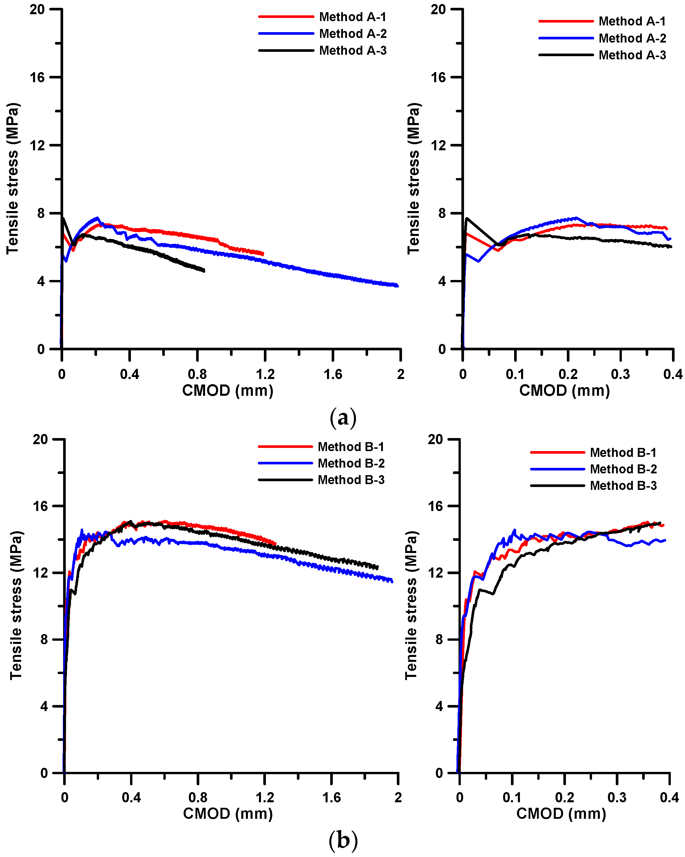
2.3. Test Results
3. Determination of the Post-Cracking Tensile Behavior
3.1. Methodology
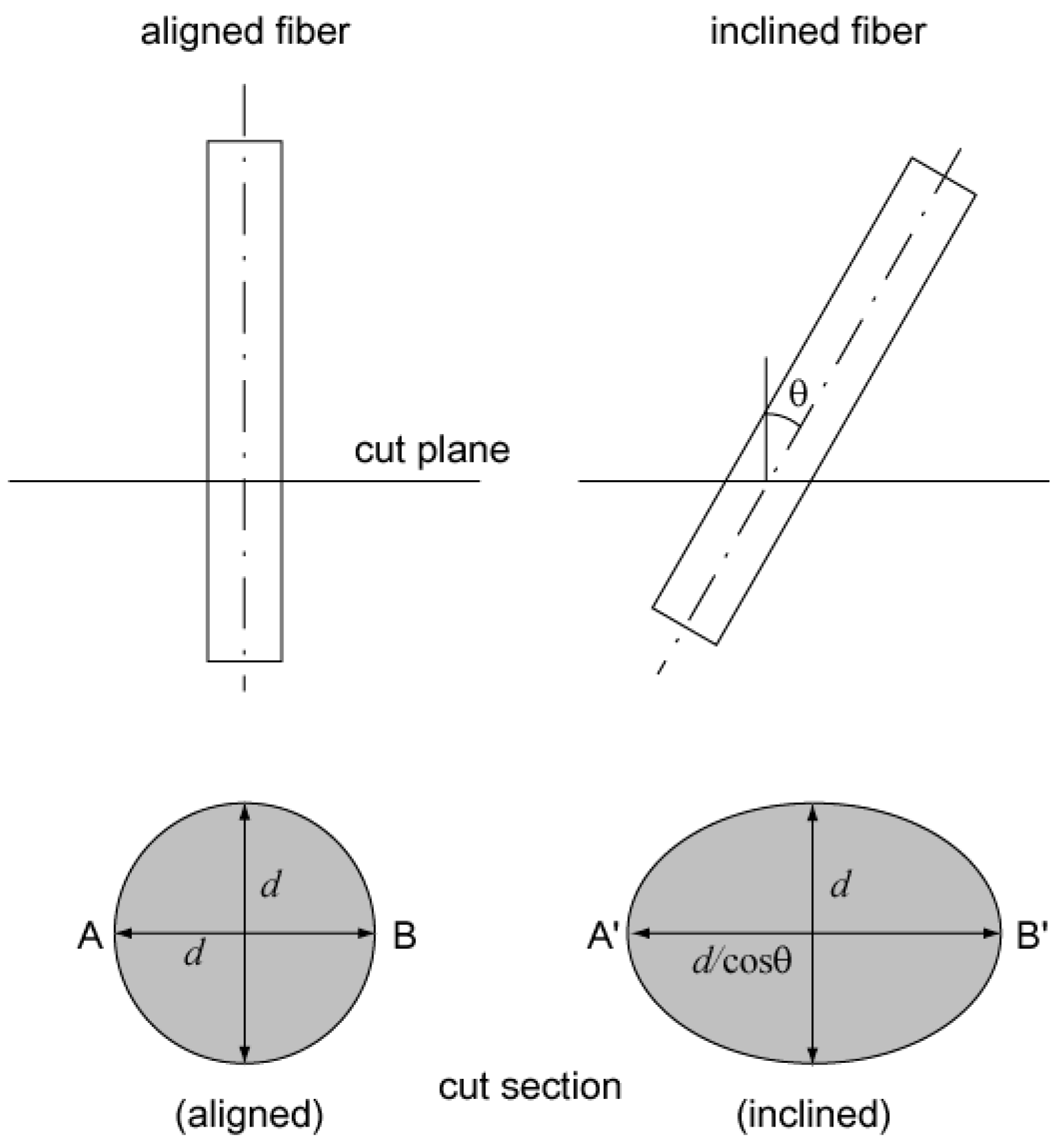
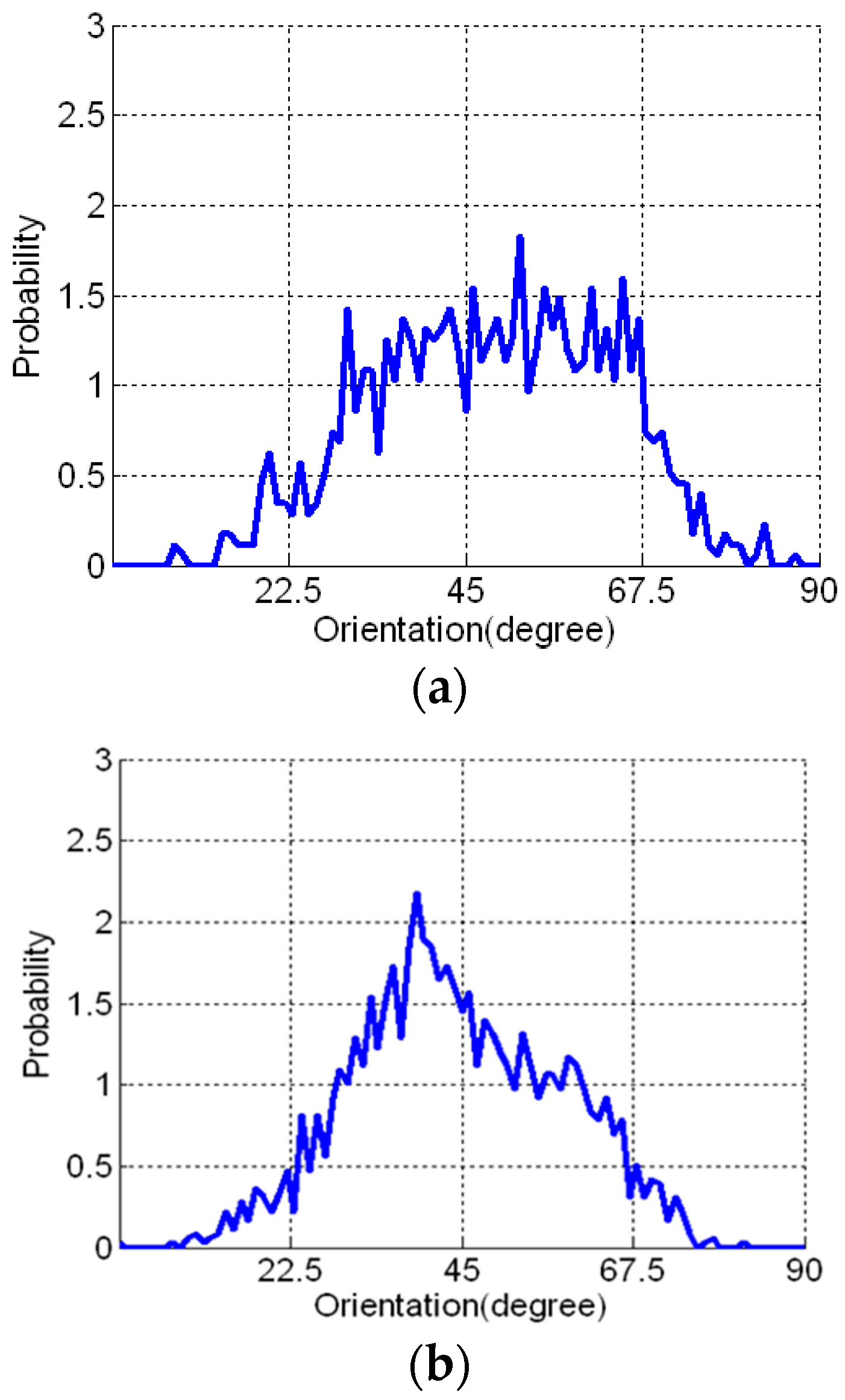
3.2. Determination of Probability Density Distribution of Fiber Orientation
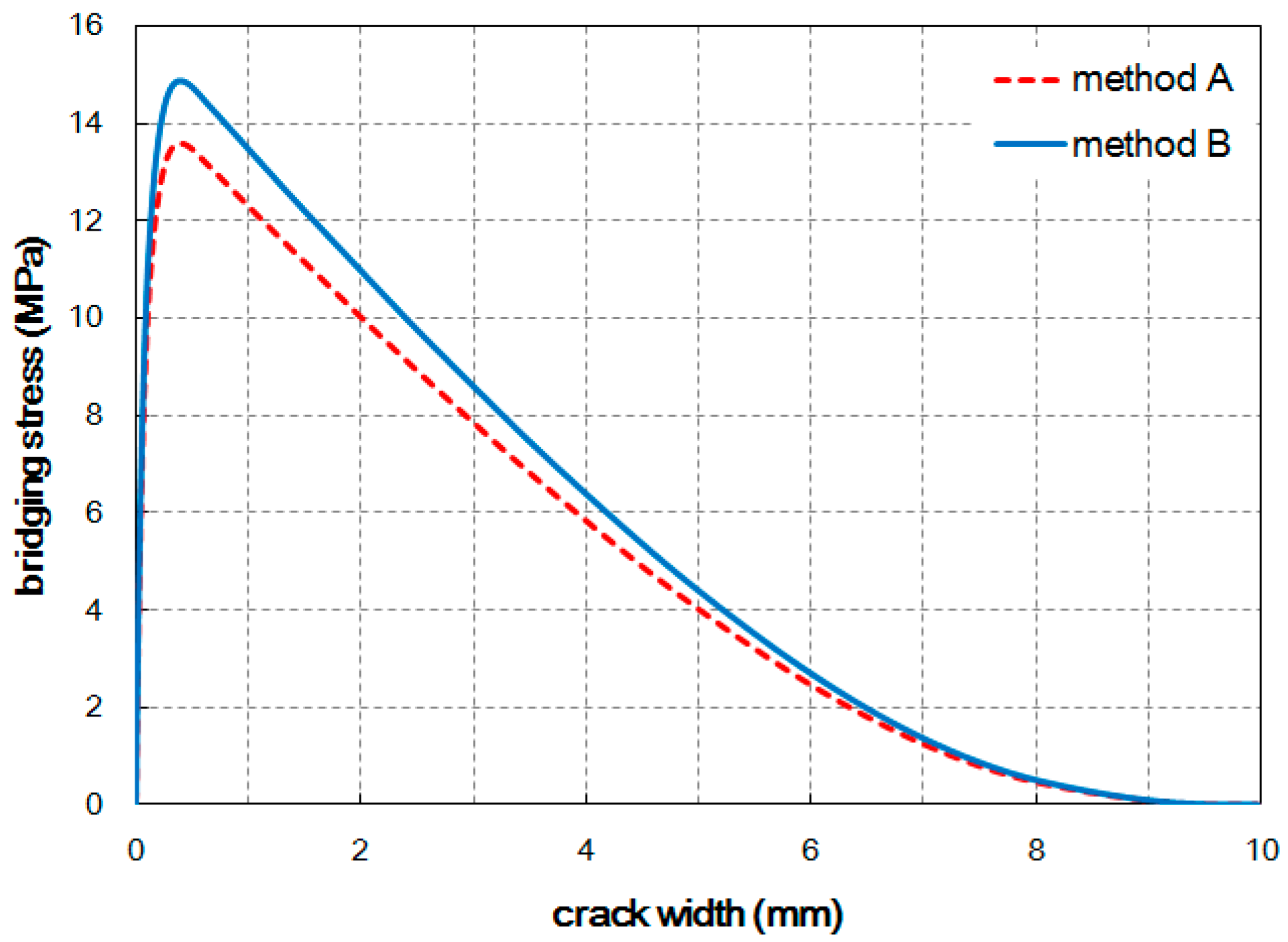
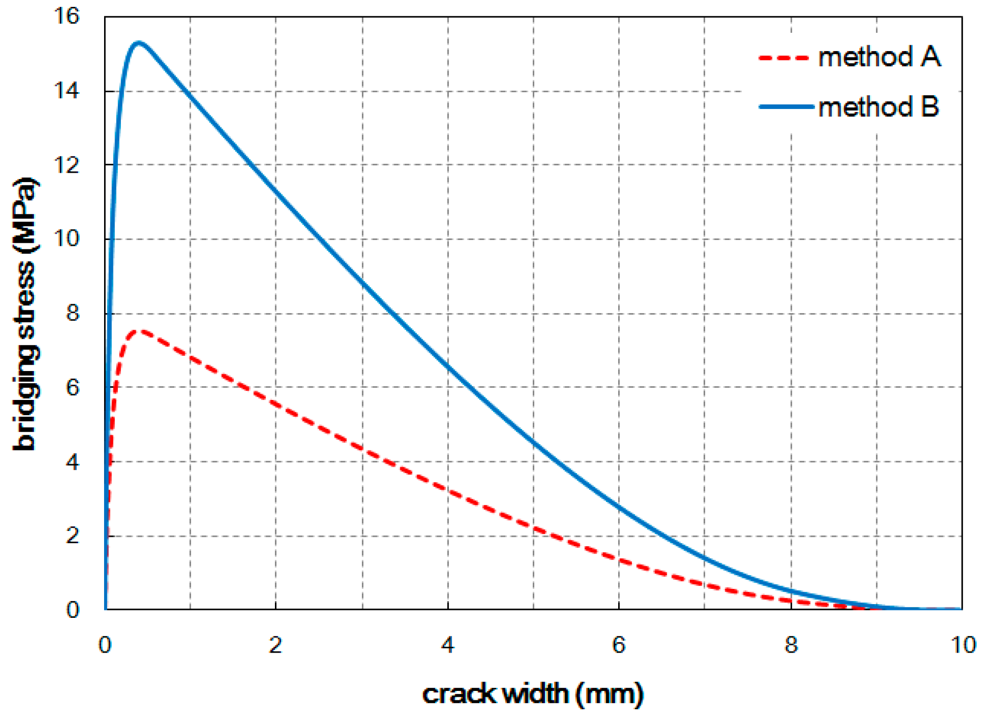
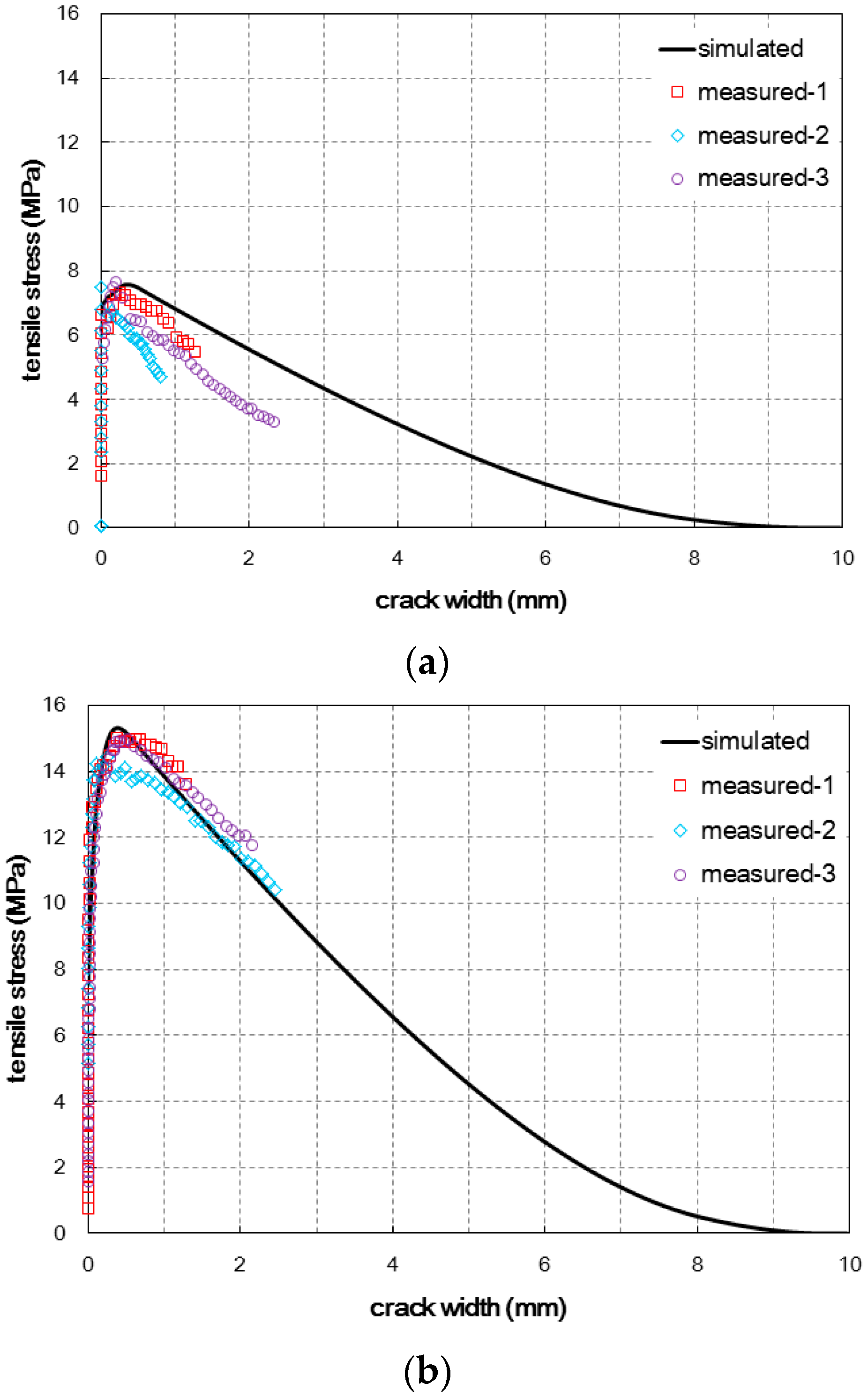
3.3. Estimation of Post-Cracking Tensile Behavior
4. Conclusions
Acknowledgments
Author Contributions
Conflicts of Interest
References
- Richard, P.; Cheyrezy, M. Composition of reactive powder concrete. Cem. Concr. Res. 1995, 25, 1501–1511. [Google Scholar] [CrossRef]
- Bonneau, O.; Lachemi, M.; Dallaire, E.; Dugat, J.; Aitcin, P.C. Mechanical properties and durability of two industrial reactive powder concretes. ACI Mater. J. 1997, 94, 286–290. [Google Scholar]
- Park, J.J.; Kang, S.T.; Koh, K.T.; Kim, S.W. Influence of the ingredients on the compressive strength of UHPC as a fundamental study to optimize the mixing proportion. In Proceedings of the Second International Symposium on Ultra High Performance Concrete, Kassel, Germany, 5–7 March 2008; pp. 105–112.
- Graybeal, B.; Davis, M. Cylinder or cube: Strength testing of 80 to 200 MPa (116 to 29 ksi) Ultra-High-Performance-Fiber-Reinforced Concrete. ACI Mater. J. 2008, 105, 603–609. [Google Scholar]
- Jungwirth, J.; Muttoni, A. Structural behavior of tension members in Ultra High Performance Concrete. In Proceedings of the International Symposium on Ultra High Performance Concrete, Kassel, Germany, 13–15 September 2004; pp. 546–553.
- Yoo, D.Y.; Lee, J.H.; Yoon, Y.S. Effect of fiber content on mechanical and fracture properties of Ultra High Performance Fiber reinforced cementitious composites. Compos. Struct. 2013, 106, 742–753. [Google Scholar] [CrossRef]
- Kang, S.T.; Lee, Y.; Park, Y.D.; Kim, J.K. Tensile fracture properties of an Ultra High Performance Fiber Reinforced Concrete (UHPFRC) with steel fiber. Compos. Struct. 2010, 92, 61–71. [Google Scholar] [CrossRef]
- Park, S.H.; Kim, D.J.; Ryu, G.S.; Koh, K.T. Tensile behavior of Ultra High Performance Hybrid Fiber Reinforced Concrete. Cem. Concr. Compos. 2012, 34, 172–184. [Google Scholar] [CrossRef]
- Wuest, J.; Denarié, E.; Brühwiler, E. Model for predicting the UHPFRC tensile hardening response. In Proceedings of the Second International Symposium on Ultra High Performance Concrete, Kassel, Germany, 5–7 March 2008; pp. 153–160.
- Naaman, A.E. A Statistical Theory of Strength for Fiber Reinforced Concrete. Ph.D. Thesis, Massacusetts Institute of Technology, Cambridge, MA, USA, 1972. [Google Scholar]
- Swamy, R.N.; Mangat, P.S.; Rao, C.V.S.K. The mechanics of fiber reinforcement of cement matrices. In An International Symposium: Fiber Reinforced Concrete; ACI SP-44: Detroit, MI, USA, 1974; pp. 1–28. [Google Scholar]
- Mai, Y.M. Strength and fracture properties of asbestos-cement mortar composites. J. Mater. Sci. 1979, 14, 2091–2102. [Google Scholar] [CrossRef]
- Rizzuti, L.; Bencardino, F. Effects of fibre volume fraction on the compressive and flexural experimental behaviour of SFRC. Contem. Eng. Sci. 2014, 7, 379–390. [Google Scholar] [CrossRef]
- Bencardino, F.; Rizzuti, L.; Spadea, G.; Swamy, R.N. Experimental evaluation of fiber reinforced concrete fracture properties. Compos. Part B Eng. 2010, 41, 17–24. [Google Scholar] [CrossRef]
- Naaman, A.E. High performance fiber reinforced cement composites. In Proceedings of the IABSE Symposium on Concrete Structures for the Future, Paris, France, 2–4 September 1987; pp. 371–376.
- Bencardino, F. Mechanical parameters and post-cracking behaviour of HPFRC according to three-point and four-point bending test. Adv. Civil Eng. 2013, 2013, 179712. [Google Scholar] [CrossRef]
- Johnson, C.D. Steel fiber reinforced mortar and concrete: A review of mechanical properties. In An International Symposium: Fiber Reinforced Concrete; ACI SP-44: Detroit, MI, USA, 1974; pp. 127–142. [Google Scholar]
- Swamy, R.N.; Stavrides, H. Some properties of high workability steel fiber reinforced concrete by electro-magnetic method. In Fibre Reinforced Cement and Concrete; Neville, A.M., Ed.; Construction Press Ltd.: Lancaster, UK, 1975; pp. 197–208. [Google Scholar]
- Markovic, I. High-Performance Hybrid-Fiber Concrete-Development and Utilization. Ph.D. Thesis, Delft University of Technology, Delft, The Netherlands, 2006. [Google Scholar]
- Ferrara, L.; di Prisco, M.; Lamperti, M.G.L. Identification of the stress-crack opening behavior of HPFRCC: The role of flow-induced fiber orientation. In Proceedings of FraMCoS-7; IA-FraMCoS: Jeju, Korea, 2010; Volume 3, pp. 1541–1550. [Google Scholar]
- Kang, S.T.; Kim, J.K. The relation between fiber orientation and tensile behavior in an Ultra High Performance Fiber Reinforced Cementitious Composites (UHPFRCC). Cem. Concr. Res. 2010, 41, 1001–1014. [Google Scholar] [CrossRef]
- Kwon, S.H.; Kang, S.T.; Lee, B.Y.; Kim, J.K. The variation of flow-dependent tensile behavior in radial flow dominant placing of Ultra High Performance Fiber Reinforced Cementitious Composites (UHPFRCC). Constr. Build. Mater. 2012, 33, 109–121. [Google Scholar] [CrossRef]
- Association Française de Génie Civil. Ultra High Performance Fiber-Reinforced Concretes—Recommendation; Association Française de Génie Civil: Paris, France, 2013. [Google Scholar]
- Japan Society of Civil Engineers. Recommendations for Design and Construction of Ultra High Strength Fiber Reinforced Concrete Structures (Draft); Japan Society of Civil Engineers: Tokyo, Japan, 2006. [Google Scholar]
- Korea Concrete Institute. Ultra High Performance Concrete K-UHPC Structural Design Guideline; Korea Concrete Institute: Seoul, Korea, 2012. (In Korean) [Google Scholar]
- Simon, A.; Corvez, D.; Marchand, P. Feedback of a ten years assessment of fibre distribution using K factor concept. In Int. Symposium on Ultra-High Performance Fibre-Reinforced Concrete, Designing and Building with UHPFRC: From Innovation to Large-Scale Realizations; RILEM Publications S.A.R.L.: Marseille, France, 2013; pp. 669–678. [Google Scholar]
- Ferrara, L.; Ozyurt, N.; di Prisco, M. High mechanical performance of fibre reinforced cementitious composites: The role of “casting-flow induced” fibre orientation. Mater. Struct. 2011, 44, 109–128. [Google Scholar] [CrossRef]
- Kang, S.T.; Lee, B.Y.; Kim, J.K.; Kim, Y.Y. The effect of fibre distribution characteristics on the flexural strength of steel fibre-reinforced Ultra high strength concrete. Constr. Build. Mater. 2011, 25, 2450–2457. [Google Scholar] [CrossRef]
- Barnett, S.J.; Lataste, J.F.; Parry, T.; Millard, S.G.; Soutsos, M.N. Assessment of fibre orientation in Ultra High performance fibre reinforced concrete and its effect on flexural strength. Mater. Struct. 2010, 43, 1009–1023. [Google Scholar] [CrossRef]
- Wille, K.; Tue, N.V.; Parra-Montesinos, G.J. Fiber distribution and orientation in UHP-FRC beams and their effect on backward analysis. Mater. Struct. 2014, 47, 1825–1838. [Google Scholar] [CrossRef]
- Soroushian, P.; Lee, C.D. Distribution and orientation of fibers in steel fiber reinforced concrete. ACI Mater. J. 1990, 87, 433–439. [Google Scholar]
- Vélez-García, G.M.; Wapperom, P.; Kunc, V.; Baird, D.G.; Zink-Sharp, A. Sample preparation and image acquisition using optical-reflective microscopy in the measurement of fiber orientation in thermoplastic composites. J. Microsc. 2012, 248, 23–33. [Google Scholar] [CrossRef] [PubMed]
- Sebaibi, N.; Benzerzour, M.; Abriak, N.E. Influence of the distribution and orientation of fibers in a reinforced concrete with waste fibres and powders. Constr. Build. Mater. 2014, 65, 254–263. [Google Scholar] [CrossRef]
- Stähli, P.; Custer, R.; van Mier, J.G. On flow properties, fibre distribution, fibre orientation and flexural behaviour of FRC. Mater. Struct. 2008, 41, 189–196. [Google Scholar] [CrossRef]
- Benson, S.D.P.; Nicolaides, D.; Karihaloo, B.L. CARDIFRC—Development and mechanical properties. Part II: Fibre distribution. Mag. Concr. Res. 2005, 57, 421–432. [Google Scholar] [CrossRef]
- Wuest, J.; Denarié, E.; Brühwiler, E.; Tamarit, L.; Kocher, M.; Gallucci, E. Tomography analysis of fiber distribution and orientation in Ultra high-performance fiber-reinforced composites with high-fiber dosages. Exp. Tech. 2008, 33, 50–55. [Google Scholar] [CrossRef]
- Liu, J.; Li, C.; Liu, J.; Cui, G.; Yang, Z. Study on 3D spatial distribution of steel fibers in fiber reinforced cementitious composites through micro-CT technique. Constr. Build. Mater. 2013, 48, 656–661. [Google Scholar] [CrossRef]
- Eik, M.; Herrmann, H. Raytraced images for testing the reconstruction of fibre orientation distributions. Proc. Estonian Acad. Sci. 2012, 61, 128–136. [Google Scholar] [CrossRef]
- Eberhardt, C.; Clarke, A.; Vincent, M.; Giroud, T.; Flouret, S. Fibre-orientation measurements in short-glass-fibre composites—II: A quantitative error estimate of the 2d image analysis technique. Compos. Sci. Technol. 2001, 61, 1961–1974. [Google Scholar] [CrossRef]
- Lee, B.Y.; Kang, S.T.; Yun, H.B.; Kim, Y.Y. Improved Sectional Image Analysis Technique for Evaluating Fiber Orientations in Fiber-Reinforced Cement-Based Materials. Materials 2016, 9, 42. [Google Scholar] [CrossRef]
- Li, V.C.; Wang, Y.; Backer, S. A micromechanical model of tension-softening and bridging toughness of short random fiber reinforced brittle matrix composites. J. Mech. Phys. Solids 1991, 39, 607–625. [Google Scholar] [CrossRef]
- Lee, Y.; Kang, S.T.; Kim, J.K. Pullout behavior of inclined steel fiber in an ultra-high strength cementitious matrix. Constr. Build. Mater. 2010, 24, 2030–2041. [Google Scholar] [CrossRef]
- Karihaloo, B.L. Fracture Mechanics and Structural Concrete (Concrete Design and Construction Series); Longman Scientific & Technical: Londo, UK, 1995. [Google Scholar]
- Folgar, F.; Tucker, C.L., III. Orientation behavior of fibers in concentrated suspensions. J. Reinf. Plast. Compos. 1984, 3, 98–119. [Google Scholar] [CrossRef]
- Piggott, M.R. Short fibre polymer composites: A fracture-based theory of fibre reinforcement. J. Compos. Mater. 1994, 28, 588–606. [Google Scholar]
- Romualdi, J.P.; Mandel, J.A. Tensile strength of concrete affected by uniformly distributed and closely spaced short lengths of wire reinforcement. J. Am. Concr. Inst. 1964, 61, 657–671. [Google Scholar]


| Item | Specific Surface Area (cm2/g) | Density (g/cm3) | Ig.loss (%) | Chemical Composition (%) | |||||
|---|---|---|---|---|---|---|---|---|---|
| SiO2 | Al2O3 | Fe2O3 | CaO | MgO | SO3 | ||||
| Cement | 3413 | 3.15 | 1.40 | 21.01 | 6.40 | 3.12 | 61.33 | 3.02 | 2.3 |
| Silica fume | 200,000 | 2.10 | 1.50 | 96.00 | 0.25 | 0.12 | 0.38 | 0.1 | - |
| Unit Mass (kg/m3) | ||||||
|---|---|---|---|---|---|---|
| Cement | Silica Fume | Sand | Filler | WRA * | Water | Steel Fiber |
| 771 | 193 | 848 | 231 | 46.3 | 160 | 156 |
| Specimen | At First Cracking | At Ultimate Stress | ||
|---|---|---|---|---|
| Stress (MPa) | CMOD (mm) | Stress (MPa) | CMOD (mm) | |
| Method A-1 | 6.79 | 0.007 | 7.34 | 0.249 |
| Method A-2 | 5.56 | 0.007 | 7.73 | 0.215 |
| Method A-3 | 7.70 | 0.008 | 7.70 | 0.008 |
| Average | 6.68 | 0.007 | 7.59 | 0.157 |
| St. dev. | 1.07 | 0.001 | 0.217 | 0.130 |
| Method B-1 | 8.69 | 0.008 | 15.10 | 0.601 |
| Method B-2 | 8.08 | 0.008 | 14.58 | 0.109 |
| Method B-3 | 5.88 | 0.006 | 15.09 | 0.397 |
| Average | 7.55 | 0.007 | 14.92 | 0.369 |
| St. dev. | 1.48 | 0.001 | 0.297 | 0.247 |
| Specimen | The Number of Total Fibers Detected | The Number of Fibers per Unit Area (Nf/mm2) | (Equation (4)) | |||
|---|---|---|---|---|---|---|
| Equation (5) | Equation (7) | |||||
| Method A | 1 | 821 | 0.205 | 0.418 | 0.322 | 0.620 |
| 2 | 988 | 0.247 | 0.475 | 0.388 | 0.667 | |
| 3 | 920 | 0.230 | 0.448 | 0.361 | 0.646 | |
| Mean | 910 | 0.227 | 0.447 | 0.357 | 0.645 | |
| Method B | 1 | 1842 | 0.406 | 0.501 | 0.723 | 0.692 |
| 2 | 1927 | 0.481 | 0.521 | 0.757 | 0.707 | |
| 3 | 1847 | 0.461 | 0.572 | 0.725 | 0.745 | |
| Mean | 1872 | 0.468 | 0.531 | 0.735 | 0.715 | |
| Number of Pixels in the Diameter of the Fiber | Fiber Orientation Angle (°) | ||||
|---|---|---|---|---|---|
| 0 | 15 | 30 | 45 | 60 | |
| 5 | 22.2 | 41.2 | 43.2 | 49.8 | 62.3 |
| 25 | 6.6 | 18.7 | 30.2 | 45.7 | 59.9 |
| 50 | 4.3 | 14.5 | 29.6 | 44.4 | 59.6 |
| 100 | 1.7 | 14.7 | 29.9 | 44.9 | 59.9 |
| Component | Parameter | Value | Description | |
|---|---|---|---|---|
| Material properties | Matrix | 45 | Elastic modulus (GPa) | |
| 0.2 | Poisson’s ratio | |||
| Fiber | 200 | Elastic modulus (GPa) | ||
| 0.3 | Poisson’s ratio | |||
| 6.8 | Apparent maximum bond strength (MPa) | |||
| 6.8 | Apparent frictional bond strength (MPa) | |||
| For ascending branch of the pullout behavior | 1.6 | Snubbing friction coefficient | ||
| 1.8 | Spalling coefficient | |||
| 5 | Parameters describing slip coefficient | |||
| 0.4 | ||||
| For descending branch of the pullout behavior | 0.05 | Parameters related to the shape of the branch | ||
| 1.0 | ||||
© 2016 by the authors; licensee MDPI, Basel, Switzerland. This article is an open access article distributed under the terms and conditions of the Creative Commons Attribution (CC-BY) license (http://creativecommons.org/licenses/by/4.0/).
Share and Cite
Choi, M.S.; Kang, S.-T.; Lee, B.Y.; Koh, K.-T.; Ryu, G.-S. Improvement in Predicting the Post-Cracking Tensile Behavior of Ultra-High Performance Cementitious Composites Based on Fiber Orientation Distribution. Materials 2016, 9, 829. https://doi.org/10.3390/ma9100829
Choi MS, Kang S-T, Lee BY, Koh K-T, Ryu G-S. Improvement in Predicting the Post-Cracking Tensile Behavior of Ultra-High Performance Cementitious Composites Based on Fiber Orientation Distribution. Materials. 2016; 9(10):829. https://doi.org/10.3390/ma9100829
Chicago/Turabian StyleChoi, Myoung Sung, Su-Tae Kang, Bang Yeon Lee, Kyeong-Taek Koh, and Gum-Sung Ryu. 2016. "Improvement in Predicting the Post-Cracking Tensile Behavior of Ultra-High Performance Cementitious Composites Based on Fiber Orientation Distribution" Materials 9, no. 10: 829. https://doi.org/10.3390/ma9100829
APA StyleChoi, M. S., Kang, S.-T., Lee, B. Y., Koh, K.-T., & Ryu, G.-S. (2016). Improvement in Predicting the Post-Cracking Tensile Behavior of Ultra-High Performance Cementitious Composites Based on Fiber Orientation Distribution. Materials, 9(10), 829. https://doi.org/10.3390/ma9100829